{"cells":[{"metadata":{"_uuid":"75eb87dace7492bfe684b08bb0d77f8bbcb4f3ce"},"cell_type":"markdown","source":"This kernel was forked from \"Fast.ai Machine Learning Lesson 1\", with my own personal notes added in.\n\nSource: https://github.com/fastai/fastai/blob/master/courses/ml1/lesson1-rf.ipynb\n\nBased on notebook version: bbcd4e0\n\nCourse page: http://course.fast.ai/ml.html"},{"metadata":{"_uuid":"16b37a420a8bbda6aa8fbe9cfde6a581104e55f5"},"cell_type":"markdown","source":"# Intro to Random Forests"},{"metadata":{"_uuid":"8e84d3d4fc5d0a5aa8d89c0065a59182de4e92aa"},"cell_type":"markdown","source":"## About this course"},{"metadata":{"_uuid":"3fe42709606dfcf989fe695761dc62756dffe7a1"},"cell_type":"markdown","source":"### Teaching approach"},{"metadata":{"_uuid":"3d42a5741f559dda969f2ee5ebed6dd952eb19a1"},"cell_type":"markdown","source":"This course is being taught by Jeremy Howard, and was developed by Jeremy along with Rachel Thomas. Rachel has been dealing with a life-threatening illness so will not be teaching as originally planned this year.\n\nJeremy has worked in a number of different areas - feel free to ask about anything that he might be able to help you with at any time, even if not directly related to the current topic:\n\n- Management consultant (McKinsey; AT Kearney)\n- Self-funded startup entrepreneur (Fastmail: first consumer synchronized email; Optimal Decisions: first optimized insurance pricing)\n- VC-funded startup entrepreneur: (Kaggle; Enlitic: first deep-learning medical company)"},{"metadata":{"_uuid":"abed84c2ece71dac3c394fb55eb393acec64aa5a"},"cell_type":"markdown","source":"I'll be using a *top-down* teaching method, which is different from how most math courses operate. Typically, in a *bottom-up* approach, you first learn all the separate components you will be using, and then you gradually build them up into more complex structures. The problems with this are that students often lose motivation, don't have a sense of the \"big picture\", and don't know what they'll need.\n\nIf you took the fast.ai deep learning course, that is what we used. You can hear more about my teaching philosophy [in this blog post](http://www.fast.ai/2016/10/08/teaching-philosophy/) or [in this talk](https://vimeo.com/214233053).\n\nHarvard Professor David Perkins has a book, [Making Learning Whole](https://www.amazon.com/Making-Learning-Whole-Principles-Transform/dp/0470633719) in which he uses baseball as an analogy. We don't require kids to memorize all the rules of baseball and understand all the technical details before we let them play the game. Rather, they start playing with a just general sense of it, and then gradually learn more rules/details as time goes on.\n\nAll that to say, don't worry if you don't understand everything at first! You're not supposed to. We will start using some \"black boxes\" such as random forests that haven't yet been explained in detail, and then we'll dig into the lower level details later.\n\nTo start, focus on what things DO, not what they ARE."},{"metadata":{"_uuid":"59c1f5aabb15ea4f417efbfd81637f94774e2bce"},"cell_type":"markdown","source":"### Your practice"},{"metadata":{"_uuid":"2e927a38965bcaf35157faca4f7976f1306ebddc"},"cell_type":"markdown","source":"People learn by:\n1. **doing** (coding and building)\n2. **explaining** what they've learned (by writing or helping others)\n\nTherefore, we suggest that you practice these skills on Kaggle by:\n1. Entering competitions (*doing*)\n2. Creating Kaggle kernels (*explaining*)\n\nIt's OK if you don't get good competition ranks or any kernel votes at first - that's totally normal! Just try to keep improving every day, and you'll see the results over time."},{"metadata":{"_uuid":"a8a3a0b6bb0bfee114a06fd91bf7763c6c53344c"},"cell_type":"markdown","source":"To get better at technical writing, study the top ranked Kaggle kernels from past competitions, and read posts from well-regarded technical bloggers. Some good role models include:\n\n- [Peter Norvig](http://nbviewer.jupyter.org/url/norvig.com/ipython/ProbabilityParadox.ipynb) (more [here](http://norvig.com/ipython/))\n- [Stephen Merity](https://smerity.com/articles/2017/deepcoder_and_ai_hype.html)\n- [Julia Evans](https://codewords.recurse.com/issues/five/why-do-neural-networks-think-a-panda-is-a-vulture) (more [here](https://jvns.ca/blog/2014/08/12/what-happens-if-you-write-a-tcp-stack-in-python/))\n- [Julia Ferraioli](http://blog.juliaferraioli.com/2016/02/exploring-world-using-vision-twilio.html)\n- [Edwin Chen](http://blog.echen.me/2014/10/07/moving-beyond-ctr-better-recommendations-through-human-evaluation/)\n- [Slav Ivanov](https://blog.slavv.com/picking-an-optimizer-for-style-transfer-86e7b8cba84b) (fast.ai student)\n- [Brad Kenstler](https://hackernoon.com/non-artistic-style-transfer-or-how-to-draw-kanye-using-captain-picards-face-c4a50256b814) (fast.ai and USF MSAN student)"},{"metadata":{"_uuid":"c24c191f97202dd6d006d1cf9aa1e98c4f426c13"},"cell_type":"markdown","source":"### Books"},{"metadata":{"_uuid":"32dfb5b4ef4d9ddfb71ceddcee6f8a68ae46d59a"},"cell_type":"markdown","source":"The more familiarity you have with numeric programming in Python, the better. If you're looking to improve in this area, we strongly suggest Wes McKinney's [Python for Data Analysis, 2nd ed](https://www.amazon.com/Python-Data-Analysis-Wrangling-IPython/dp/1491957662/ref=asap_bc?ie=UTF8).\n\nFor machine learning with Python, we recommend:\n\n- [Introduction to Machine Learning with Python](https://www.amazon.com/Introduction-Machine-Learning-Andreas-Mueller/dp/1449369413): From one of the scikit-learn authors, which is the main library we'll be using\n- [Python Machine Learning: Machine Learning and Deep Learning with Python, scikit-learn, and TensorFlow, 2nd Edition](https://www.amazon.com/Python-Machine-Learning-scikit-learn-TensorFlow/dp/1787125939/ref=dp_ob_title_bk): New version of a very successful book. A lot of the new material however covers deep learning in Tensorflow, which isn't relevant to this course\n- [Hands-On Machine Learning with Scikit-Learn and TensorFlow](https://www.amazon.com/Hands-Machine-Learning-Scikit-Learn-TensorFlow/dp/1491962291/ref=pd_lpo_sbs_14_t_0?_encoding=UTF8&psc=1&refRID=MBV2QMFH3EZ6B3YBY40K)\n"},{"metadata":{"_uuid":"82241a836b6bbb4ba643517a509e330fbd266a5a"},"cell_type":"markdown","source":"### Syllabus in brief"},{"metadata":{"_uuid":"cb2cb72f33559cc8c8088f796aad70eaa38732e3"},"cell_type":"markdown","source":"Depending on time and class interests, we'll cover something like (not necessarily in this order):\n\n- Train vs test\n - Effective validation set construction\n- Trees and ensembles\n - Creating random forests\n - Interpreting random forests\n- What is ML? Why do we use it?\n - What makes a good ML project?\n - Structured vs unstructured data\n - Examples of failures/mistakes\n- Feature engineering\n - Domain specific - dates, URLs, text\n - Embeddings / latent factors\n- Regularized models trained with SGD\n - GLMs, Elasticnet, etc (NB: see what James covered)\n- Basic neural nets\n - PyTorch\n - Broadcasting, Matrix Multiplication\n - Training loop, backpropagation\n- KNN\n- CV / bootstrap (Diabetes data set?)\n- Ethical considerations"},{"metadata":{"_uuid":"eb292c111db17f30a7722dfad1878b8a244bb9b8"},"cell_type":"markdown","source":"Skip:\n\n- Dimensionality reduction\n- Interactions\n- Monitoring training\n- Collaborative filtering\n- Momentum and LR annealing\n"},{"metadata":{"_uuid":"a5cccd7ec19f6d4c6b05bfc47ca02778ddc3de37"},"cell_type":"markdown","source":"## Imports"},{"metadata":{"trusted":true,"_uuid":"d4ebff0d03af59c9f91924f07e273641c62ca3bf"},"cell_type":"code","source":"!pip install git+https://github.com/fastai/fastai@2e1ccb58121dc648751e2109fc0fbf6925aa8887\n\n!apt update && apt install -y libsm6 libxext6","execution_count":null,"outputs":[]},{"metadata":{"trusted":true,"_uuid":"c60ee5a1bbe5e8768193cb46ecc555a613f00dfb"},"cell_type":"code","source":"#Load \"autoreload\" extension for automatically reloading imported modules before each code execution\n%load_ext autoreload\n#Reload all modules except those specified in %aimport (none in this case)\n%autoreload 2\n\n#Display matplotlib plots\n%matplotlib inline","execution_count":null,"outputs":[]},{"metadata":{"trusted":true,"_uuid":"7912257885c6ad962cda63f075bf83a079578d78"},"cell_type":"code","source":"#Import fastai modules\n#Does not follow PEP8 style (wildcard \"*\" imports)\n#\"Data science is not software engineering\", \"follow prototyping best practices\", \"interactive and iterative\"\n\n#Import all other relevant modules\nfrom fastai.imports import *\n#Import all relevant functions\nfrom fastai.structured import *\n\n#Import \"DataFrameSummary\" class which extends Pandas dataframe's describe() method\nfrom pandas_summary import DataFrameSummary\n#Import scikit-learn's classes for building random forests models (regression and classification)\nfrom sklearn.ensemble import RandomForestRegressor, RandomForestClassifier\n#Import IPython's display() function for displaying Python objects\nfrom IPython.display import display\n\n#Import scikit-learn's metrics module for measuring model performance\nfrom sklearn import metrics","execution_count":null,"outputs":[]},{"metadata":{"trusted":true,"_uuid":"941a67d4ae3a4337b3a7aa42d8afa141cd83cc32"},"cell_type":"code","source":"#Fix\nimport feather","execution_count":null,"outputs":[]},{"metadata":{"trusted":true,"_uuid":"1553fc50ca89000c71ab93fdb9a3e3f84fdd8c50"},"cell_type":"code","source":"#Path for directory containing input data\nPATH = \"../input/\"","execution_count":null,"outputs":[]},{"metadata":{"trusted":true,"_uuid":"3bb2c655c18aa1b54fba2cc8d425d37eb8adf596"},"cell_type":"code","source":"#!ls: execute shell command in notebook (list files in current working directory)\n#{PATH}: pass python variable (PATH) into shell command\n!ls {PATH}","execution_count":null,"outputs":[]},{"metadata":{"_uuid":"60e650bdee9ad8be88cb10811015578755f28fc9"},"cell_type":"markdown","source":"# Introduction to *Blue Book for Bulldozers*"},{"metadata":{"_uuid":"9d3292c23abdf11b58850f02555392cd38c98400"},"cell_type":"markdown","source":"## About..."},{"metadata":{"_uuid":"11121596be394c8cedbee7dbfbe53311e9f598ad"},"cell_type":"markdown","source":"### ...our teaching"},{"metadata":{"_uuid":"f805a7c8465c43c4fda332732daee0f7354c0f63"},"cell_type":"markdown","source":"At fast.ai we have a distinctive [teaching philosophy](http://www.fast.ai/2016/10/08/teaching-philosophy/) of [\"the whole game\"](https://www.amazon.com/Making-Learning-Whole-Principles-Transform/dp/0470633719/ref=sr_1_1?ie=UTF8&qid=1505094653). This is different from how most traditional math & technical courses are taught, where you have to learn all the individual elements before you can combine them (Harvard professor David Perkins call this *elementitis*), but it is similar to how topics like *driving* and *baseball* are taught. That is, you can start driving without [knowing how an internal combustion engine works](https://medium.com/towards-data-science/thoughts-after-taking-the-deeplearning-ai-courses-8568f132153), and children begin playing baseball before they learn all the formal rules."},{"metadata":{"_uuid":"11bb1e0cbc6380540862d6739f6c3ec9927af911"},"cell_type":"markdown","source":"### ...our approach to machine learning"},{"metadata":{"_uuid":"98b864b8140a971268c250e80f0fd0e9c87437a6"},"cell_type":"markdown","source":"Most machine learning courses will throw at you dozens of different algorithms, with a brief technical description of the math behind them, and maybe a toy example. You're left confused by the enormous range of techniques shown and have little practical understanding of how to apply them.\n\nThe good news is that modern machine learning can be distilled down to a couple of key techniques that are of very wide applicability. Recent studies have shown that the vast majority of datasets can be best modeled with just two methods:\n\n- *Ensembles of decision trees* (i.e. Random Forests and Gradient Boosting Machines), mainly for structured data (such as you might find in a database table at most companies)\n- *Multi-layered neural networks learnt with SGD* (i.e. shallow and/or deep learning), mainly for unstructured data (such as audio, vision, and natural language)\n\nIn this course we'll be doing a deep dive into random forests, and simple models learnt with SGD. You'll be learning about gradient boosting and deep learning in part 2."},{"metadata":{"_uuid":"3cb4ea4b6bff3d41d57250690d797551a0d0f9b9"},"cell_type":"markdown","source":"### ...this dataset"},{"metadata":{"_uuid":"c30037666dc0f823cb224b0b62dcc2adc6f3ee63"},"cell_type":"markdown","source":"We will be looking at the Blue Book for Bulldozers Kaggle Competition: \"The goal of the contest is to predict the sale price of a particular piece of heavy equiment at auction based on it's usage, equipment type, and configuaration. The data is sourced from auction result postings and includes information on usage and equipment configurations.\"\n\nThis is a very common type of dataset and prediciton problem, and similar to what you may see in your project or workplace."},{"metadata":{"_uuid":"a2650e53030077d3baf8184654a74f6540c4b4f7"},"cell_type":"markdown","source":"### ...Kaggle Competitions"},{"metadata":{"_uuid":"02ede64c1e83f7316294ee48a933648f56be62e4"},"cell_type":"markdown","source":"Kaggle is an awesome resource for aspiring data scientists or anyone looking to improve their machine learning skills. There is nothing like being able to get hands-on practice and receiving real-time feedback to help you improve your skills.\n\nKaggle provides:\n\n1. Interesting data sets\n2. Feedback on how you're doing\n3. A leader board to see what's good, what's possible, and what's state-of-art.\n4. Blog posts by winning contestants share useful tips and techniques."},{"metadata":{"_uuid":"5f0189251c18287203a4b95def8898ea89259af2"},"cell_type":"markdown","source":"## The data"},{"metadata":{"_uuid":"b49848148c341837151d7456720f0b2bff36d987"},"cell_type":"markdown","source":"### Look at the data"},{"metadata":{"_uuid":"1149856226dac1e27881a3677aeae51702569742"},"cell_type":"markdown","source":"Kaggle provides info about some of the fields of our dataset; on the [Kaggle Data info](https://www.kaggle.com/c/bluebook-for-bulldozers/data) page they say the following:\n\nFor this competition, you are predicting the sale price of bulldozers sold at auctions. The data for this competition is split into three parts:\n\n- **Train.csv** is the training set, which contains data through the end of 2011.\n- **Valid.csv** is the validation set, which contains data from January 1, 2012 - April 30, 2012 You make predictions on this set throughout the majority of the competition. Your score on this set is used to create the public leaderboard.\n- **Test.csv** is the test set, which won't be released until the last week of the competition. It contains data from May 1, 2012 - November 2012. Your score on the test set determines your final rank for the competition.\n\nThe key fields are in train.csv are:\n\n- SalesID: the uniue identifier of the sale\n- MachineID: the unique identifier of a machine. A machine can be sold multiple times\n- saleprice: what the machine sold for at auction (only provided in train.csv)\n- saledate: the date of the sale"},{"metadata":{"_uuid":"d3469b1c42052c108e3ba200f42c5adbcb54381d"},"cell_type":"markdown","source":"*Question*\n\nWhat stands out to you from the above description? What needs to be true of our training and validation sets?"},{"metadata":{"trusted":true,"_uuid":"41b261c8d694c70e60aaa1a2fabec6d53511e551"},"cell_type":"code","source":"#We have already imported pandas as pd in \"from fastai.imports import *\"\n#\"low_memory=False\": Avoid mixed type inference (from internally processing the csv file in chunks)\n#\"parse_dates=[\"saledate\"]\": parse the \"saledate\" column as a date column\ndf_raw = pd.read_csv(f'{PATH}train/Train.csv', low_memory=False, parse_dates=[\"saledate\"])","execution_count":null,"outputs":[]},{"metadata":{"_uuid":"2ed669a86a8399ca2ee8824887afb9834f809164"},"cell_type":"markdown","source":"In any sort of data science work, it's **important to look at your data**, to make sure you understand the format, how it's stored, what type of values it holds, etc. Even if you've read descriptions about your data, the actual data may not be what you expect."},{"metadata":{"trusted":true,"_uuid":"4ed9f5f5e4fe6cdb29a8ca41679a4b0374d7cfe2"},"cell_type":"code","source":"#Function for displaying all the columns of the dataframe\ndef display_all(df):\n with pd.option_context(\"display.max_rows\", 1000, \"display.max_columns\", 1000): \n display(df)","execution_count":null,"outputs":[]},{"metadata":{"trusted":true,"_uuid":"8cd2ed4942a5bb79bf8592f3c956321ea0d25c8a"},"cell_type":"code","source":"#We want to have an overview of all the variables\n#Take the last 5 (default value) rows in the dataframe, transpose and display it\ndisplay_all(df_raw.tail().T)","execution_count":null,"outputs":[]},{"metadata":{"trusted":true,"_uuid":"cd4243ff25dbe4528b2011b8358123999199398b","scrolled":true},"cell_type":"code","source":"#Get descriptive statistics for all columns\ndisplay_all(df_raw.describe(include='all').T)","execution_count":null,"outputs":[]},{"metadata":{"_uuid":"84a5bcad9c7e0c147ed4c77be3d8c40190a24581"},"cell_type":"markdown","source":"\"Question: Should you never look at the data because of the risk of overfit? [33:08] We want to find out at least enough to know that we have managed to imported okay, but tend not to really study it at all at this point, because we do not want to make too many assumptions about it. Many books say to do a lot of exploratory data analysis (EDA) first. We will learn machine learning driven EDA today.\""},{"metadata":{"_uuid":"b8f6e907ba48aa52f5b56b64c2beafffc5b6c6be"},"cell_type":"markdown","source":"It's important to note what metric is being used for a project. Generally, selecting the metric(s) is an important part of the project setup. However, in this case Kaggle tells us what metric to use: RMSLE (root mean squared log error) between the actual and predicted auction prices. Therefore we take the log of the prices, so that RMSE will give us what we need."},{"metadata":{"_uuid":"7ed60b362c93e049677888fb3e9c261581f92cdb"},"cell_type":"markdown","source":"\"The reason we use log is because generally, you care not so much about missing by $10 but missing by 10. So if it was a $1000,000 item and you are $100,000 off or if it was a $10,000 item and you are $1,000 off — we would consider those equivalent scale issues.\""},{"metadata":{"trusted":true,"_uuid":"35cfe43dafa4d604ca53dfdc6c03e5321ca6e815"},"cell_type":"code","source":"#Get natural logarithm of SalePrice\ndf_raw.SalePrice = np.log(df_raw.SalePrice)","execution_count":null,"outputs":[]},{"metadata":{"_uuid":"0cc071a293471e10537a6e50388365af06c7cda5"},"cell_type":"markdown","source":"### Initial processing"},{"metadata":{"_uuid":"b8d523c0cb327844baced5882b0cbd0d2b473892"},"cell_type":"markdown","source":"\"Random forest is a universal machine learning technique.\n\n- It can predict something that can be of any kind — it could be a category (classification), a continuous variable (regression).\n- It can predict with columns of any kind — pixels, zip codes, revenues, etc (i.e. both structured and unstructured data).\n- It does not generally overfit too badly, and it is very easy to stop it from overfitting.\n- You do not need a separate validation set in general. It can tell you how well it generalizes even if you only have one dataset.\n- It has few, if any, statistical assumptions. It does not assume that your data is normally distributed, the relationship is linear, or you have specified interactions.\n- It requires very few pieces of feature engineering. For many different types of situation, you do not have to take the log of the data or multiply interactions together.\""},{"metadata":{"_uuid":"b21a56187fa506a15aa773f97845cf28b5c6da3d"},"cell_type":"markdown","source":"- RandomForestRegressor — regressor is a method for predicting continuous variables (i.e. regression)\n- RandomForestClassifier — classifier is a method for predicting categorical variables (i.e. classification)"},{"metadata":{"trusted":true,"_uuid":"d1442ed3373eabd82822f7d0ffe519a3f1107f8f"},"cell_type":"code","source":"#Create model object\n#n_jobs = -1: use all CPUs\nm = RandomForestRegressor(n_jobs=-1)\n#Build model\n#The following code is supposed to fail due to string values in the input data\nm.fit(df_raw.drop('SalePrice', axis=1), df_raw.SalePrice)","execution_count":null,"outputs":[]},{"metadata":{"_uuid":"5f36a0f5a3903f975140edac62652941cdc4cd24"},"cell_type":"markdown","source":"\"We have to pass numbers to most machine learning models and certainly to random forests. So step 1 is to convert everything into numbers.\""},{"metadata":{"_uuid":"b6b9a4cb48e02fb8cc57797daab06d569e8cbb01"},"cell_type":"markdown","source":"This dataset contains a mix of **continuous** and **categorical** variables.\n\nThe following method extracts particular date fields from a complete datetime for the purpose of constructing categoricals. You should always consider this feature extraction step when working with date-time. Without expanding your date-time into these additional fields, you can't capture any trend/cyclical behavior as a function of time at any of these granularities."},{"metadata":{"_uuid":"2f81cd154884ef854719751a021f4a7c03ea3f10"},"cell_type":"markdown","source":"\"Here are some of the information we can extract from date — year, month, quarter, day of month, day of week, week of year, is it a holiday? weekend? was it raining? was there a sport event that day? It really depends on what you are doing. If you are predicting soda sales in SoMa, you would probably want to know if there was a San Francisco Giants ball game that day. What is in a date is one of the most important piece of feature engineering you can do and no machine learning algorithm can tell you whether the Giants were playing that day and that it was important. So this is where you need to do feature engineering.\""},{"metadata":{"trusted":true,"_uuid":"1a7f1fe7c35ab06af3be1887069b1ba3e6b3b537"},"cell_type":"code","source":"add_datepart(df_raw, 'saledate')\ndf_raw.saleYear.head()","execution_count":null,"outputs":[]},{"metadata":{"_uuid":"b9464b2fa33182beff0ced4bac3550984bfac90f"},"cell_type":"markdown","source":"The categorical variables are currently stored as strings, which is inefficient, and doesn't provide the numeric coding required for a random forest. Therefore we call `train_cats` to convert strings to pandas categories."},{"metadata":{"_uuid":"9b2764beee2c78da1562da8210af9cbd648b6847"},"cell_type":"markdown","source":"\"Fast.ai provides a function called train_cats which creates categorical variables for everything that is a String. Behind the scenes, it creates a column that is an integer and it is going to store a mapping from the integers to the strings. train_cats is called “train” because it is training data specific. It is important that validation and test sets will use the same category mappings (in other words, if you used 1 for “high” for a training dataset, then 1 should also be for “high” in validation and test datasets). For validation and test dataset, use apply_cats instead.\""},{"metadata":{"trusted":true,"_uuid":"a4144eec5300c7ec2049f78b8c4e40224af07179"},"cell_type":"code","source":"train_cats(df_raw)","execution_count":null,"outputs":[]},{"metadata":{"_uuid":"62d77f6bc53a15291207738fc61f2f8aaab96278"},"cell_type":"markdown","source":"We can specify the order to use for categorical variables if we wish:"},{"metadata":{"trusted":true,"_uuid":"b0c368634b1ed38a90cd9e208996842e4b724ade"},"cell_type":"code","source":"df_raw.UsageBand.cat.categories","execution_count":null,"outputs":[]},{"metadata":{"trusted":true,"_uuid":"0ea5f86ac312804007cb32a8bea4539c5018355d"},"cell_type":"code","source":"df_raw.UsageBand.cat.set_categories(['High', 'Medium', 'Low'], ordered=True, inplace=True)","execution_count":null,"outputs":[]},{"metadata":{"_uuid":"fadf451e28e76844f095b462fd14f3fdcad28ba1"},"cell_type":"markdown","source":"Normally, pandas will continue displaying the text categories, while treating them as numerical data internally. Optionally, we can replace the text categories with numbers, which will make this variable non-categorical, like so:."},{"metadata":{"trusted":true,"_uuid":"f60fc234c7a93d6a3533528ab77f65786fb72c85"},"cell_type":"code","source":"df_raw.UsageBand = df_raw.UsageBand.cat.codes","execution_count":null,"outputs":[]},{"metadata":{"_uuid":"800312d593aeb1580aa44122c289ff26ee63329b"},"cell_type":"markdown","source":"We're still not quite done - for instance we have lots of missing values, which we can't pass directly to a random forest."},{"metadata":{"trusted":true,"_uuid":"b676bee8d374d5ec7893c9d2a091ab30e6a77b18"},"cell_type":"code","source":"display_all(df_raw.isnull().sum().sort_index()/len(df_raw))","execution_count":null,"outputs":[]},{"metadata":{"_uuid":"a3db805fd46e17c5031cfaf19a352c3a7003e491"},"cell_type":"markdown","source":"But let's save this file for now, since it's already in format can we be stored and accessed efficiently."},{"metadata":{"_uuid":"2149e13cc94661904124688201072920e130fd6c"},"cell_type":"markdown","source":"\"What this is going to do is to save it to disk in exactly the same basic format that it is in RAM. This is by far the fastest way to save something, and also to read it back.\""},{"metadata":{"trusted":true,"_uuid":"65ced22eac1dea3cabf530d346ec97c15bc065e0"},"cell_type":"code","source":"os.makedirs('tmp', exist_ok=True)\ndf_raw.to_feather('tmp/bulldozers-raw')","execution_count":null,"outputs":[]},{"metadata":{"_uuid":"0582df5346613907d2a9677338b20aa7f1dfc61c"},"cell_type":"markdown","source":"### Pre-processing"},{"metadata":{"_uuid":"3ac8081b051680d3d2ef9d76abec702cc3bac07f"},"cell_type":"markdown","source":"In the future we can simply read it from this fast format."},{"metadata":{"trusted":true,"_uuid":"733330a90193ab33737f7f4e1503f4163895a7ea"},"cell_type":"code","source":"df_raw = feather.read_dataframe('tmp/bulldozers-raw')","execution_count":null,"outputs":[]},{"metadata":{"_uuid":"94b5d2d8c58cff8ce877128726bdcb8c5b54a05c"},"cell_type":"markdown","source":"We'll replace categories with their numeric codes, handle missing continuous values, and split the dependent variable into a separate variable."},{"metadata":{"trusted":true,"_uuid":"ed570c9814e8ec683426a3365069d6814b8a50f9"},"cell_type":"code","source":"df, y, nas = proc_df(df_raw, 'SalePrice')","execution_count":null,"outputs":[]},{"metadata":{"trusted":true,"_uuid":"2ea1c79e863e11d27e855ea0dfa52bbd9f6c1417"},"cell_type":"code","source":"df.head()","execution_count":null,"outputs":[]},{"metadata":{"_uuid":"f99758dbfcbaa9f2ce2833aff2c772a11f2a8100"},"cell_type":"markdown","source":"We now have something we can pass to a random forest!"},{"metadata":{"_uuid":"71a55e0c8a764c9268990bccc0146df45ecff49d"},"cell_type":"markdown","source":"\"Random forests are trivially parallelizable — meaning if you have more than one CPU, you can split up the data across different CPUs and it linearly scale. So the more CPUs you have, it will divide the time it takes by that number (not exactly but roughly).\""},{"metadata":{"trusted":true,"_uuid":"4c525e4e0ef52fde0947e856d35f2f67b5b5dac1"},"cell_type":"code","source":"m = RandomForestRegressor(n_jobs=-1)\nm.fit(df, y)\nm.score(df,y)","execution_count":null,"outputs":[]},{"metadata":{"_uuid":"383c3cfdc639a7d7c22f4755c6e671f0c7920123"},"cell_type":"markdown","source":"In statistics, the coefficient of determination, denoted R2 or r2 and pronounced \"R squared\", is the proportion of the variance in the dependent variable that is predictable from the independent variable(s). https://en.wikipedia.org/wiki/Coefficient_of_determination"},{"metadata":{"_uuid":"e4d298e801f657dce378d1038adf1d418b0838f5"},"cell_type":"markdown","source":"Basics of r2: https://towardsdatascience.com/coefficient-of-determination-r-squared-explained-db32700d924e"},{"metadata":{"_uuid":"020bfeb83d420ce965a79fe106875a057e57613d"},"cell_type":"markdown","source":"Wow, an r^2 of 0.98 - that's great, right? Well, perhaps not...\n\nPossibly **the most important idea** in machine learning is that of having separate training & validation data sets. As motivation, suppose you don't divide up your data, but instead use all of it. And suppose you have lots of parameters:\n\n \n\n[Underfitting and Overfitting](https://datascience.stackexchange.com/questions/361/when-is-a-model-underfitted)\n\n\nThe error for the pictured data points is lowest for the model on the far right (the blue curve passes through the red points almost perfectly), yet it's not the best choice. Why is that? If you were to gather some new data points, they most likely would not be on that curve in the graph on the right, but would be closer to the curve in the middle graph.\n\nThis illustrates how using all our data can lead to **overfitting**. A validation set helps diagnose this problem."},{"metadata":{"trusted":true,"_uuid":"03b0ed8a3fc084f564e39fc1e6a715b213e46968"},"cell_type":"code","source":"def split_vals(a,n): return a[:n].copy(), a[n:].copy()\n\n#Set number of rows for validation set\nn_valid = 12000 # same as Kaggle's test set size\n#Remaining number of rows is used for training set\nn_trn = len(df)-n_valid\n\n#Split unprocessed dataframe\nraw_train, raw_valid = split_vals(df_raw, n_trn)\n#Split processed dataframe and series: see proc_df() function\nX_train, X_valid = split_vals(df, n_trn)\ny_train, y_valid = split_vals(y, n_trn)\n\nX_train.shape, y_train.shape, X_valid.shape","execution_count":null,"outputs":[]},{"metadata":{"_uuid":"5d8329eaf818288f6c83d52eb3d5329e963339f3"},"cell_type":"markdown","source":"# Random Forests"},{"metadata":{"_uuid":"cf8d544aa84ddf83a24b8bef5ed75720c6f443a0"},"cell_type":"markdown","source":"## Base model"},{"metadata":{"_uuid":"2ed0cf181423696c20c92934e26e70ccdd8b265b"},"cell_type":"markdown","source":"Let's try our model again, this time with separate training and validation sets."},{"metadata":{"trusted":true,"_uuid":"f6e62979fe4dabb8fd689dbc6d42bee0c9e83fee"},"cell_type":"code","source":"def rmse(x,y): return math.sqrt(((x-y)**2).mean())\n\ndef print_score(m):\n res = [rmse(m.predict(X_train), y_train), rmse(m.predict(X_valid), y_valid),\n m.score(X_train, y_train), m.score(X_valid, y_valid)]\n if hasattr(m, 'oob_score_'): res.append(m.oob_score_)\n print(res)","execution_count":null,"outputs":[]},{"metadata":{"trusted":true,"_uuid":"5d6cfd947159d73ccfe6367fd03d9dc08fa7afbe"},"cell_type":"code","source":"m = RandomForestRegressor(n_jobs=-1)\n%time m.fit(X_train, y_train)\nprint_score(m)","execution_count":null,"outputs":[]},{"metadata":{"_uuid":"92ffd14ea998497b5947bbba7ab75b6565cb146c"},"cell_type":"markdown","source":"An r^2 in the high-80's isn't bad at all (and the RMSLE puts us around rank 100 of 470 on the Kaggle leaderboard), but we can see from the validation set score that we're over-fitting badly. To understand this issue, let's simplify things down to a single small tree."},{"metadata":{"_uuid":"c999022626c8deb82e8d7a01a3c5f9fcd2ad44b7"},"cell_type":"markdown","source":"## Speeding things up"},{"metadata":{"trusted":true,"_uuid":"dba65c173a4bf520ed2ed5ded6eba3f96e2cdc53"},"cell_type":"code","source":"df_trn, y_trn, nas = proc_df(df_raw, 'SalePrice', subset=30000, na_dict=nas)\nX_train, _ = split_vals(df_trn, 20000)\ny_train, _ = split_vals(y_trn, 20000)","execution_count":null,"outputs":[]},{"metadata":{"trusted":true,"_uuid":"bc6e18f5fd17aed0c3bb8d62c7c98ad0f4bb32da"},"cell_type":"code","source":"m = RandomForestRegressor(n_jobs=-1)\n%time m.fit(X_train, y_train)\nprint_score(m)","execution_count":null,"outputs":[]},{"metadata":{"_uuid":"4647d289cbd7cdcbd31fd5ea4d5166f4ae568235"},"cell_type":"markdown","source":"## Single tree"},{"metadata":{"trusted":true,"_uuid":"9e6d17691844ef9fa50ababd87c0eb0ca5cc492c"},"cell_type":"code","source":"# n_estimators=1: one tree\n# bootstrap=False: do not use bootstrap samples\n# \" random forest randomizes bunch of things, we want to turn that off by this parameter\"\nm = RandomForestRegressor(n_estimators=1, max_depth=3, bootstrap=False, n_jobs=-1)\nm.fit(X_train, y_train)\nprint_score(m)","execution_count":null,"outputs":[]},{"metadata":{"trusted":true,"_uuid":"284184d1414693e56b10620e22b6552de028efd4"},"cell_type":"code","source":"draw_tree(m.estimators_[0], df_trn, precision=3)","execution_count":null,"outputs":[]},{"metadata":{"_uuid":"6b6e628d571c108a71d30445c17f226b5037b33f"},"cell_type":"markdown","source":"Let's see what happens if we create a bigger tree."},{"metadata":{"trusted":true,"_uuid":"b26e645cbe05163ee4f7c28b799b82b7761e3a0d"},"cell_type":"code","source":"m = RandomForestRegressor(n_estimators=1, bootstrap=False, n_jobs=-1)\nm.fit(X_train, y_train)\nprint_score(m)","execution_count":null,"outputs":[]},{"metadata":{"_uuid":"e5d97643db5fc17d1491d523353432387140f27a"},"cell_type":"markdown","source":"The training set result looks great! But the validation set is worse than our original model. This is why we need to use *bagging* of multiple trees to get more generalizable results."},{"metadata":{"_uuid":"3aa0517b0aaebe10f38795a8d70e17cb7852b1c1"},"cell_type":"markdown","source":"## Bagging"},{"metadata":{"_uuid":"d09094ea4745e94ed20fae5e38544ed9d15db8e1"},"cell_type":"markdown","source":"### Intro to bagging"},{"metadata":{"_uuid":"68442fcd7eb5f82f8a8ec2a7ce772ac41b6a815d"},"cell_type":"markdown","source":"To learn about bagging in random forests, let's start with our basic model again."},{"metadata":{"trusted":true,"_uuid":"5af941fe1827be61fd5c0bc3d6b03abc0805dcc4"},"cell_type":"code","source":"# default number of trees is 10\nm = RandomForestRegressor(n_jobs=-1)\nm.fit(X_train, y_train)\nprint_score(m)","execution_count":null,"outputs":[]},{"metadata":{"_uuid":"3a5168a933d90491ffce0bcd10fde92baecca7d5"},"cell_type":"markdown","source":"We'll grab the predictions for each individual tree, and look at one example."},{"metadata":{"trusted":true,"_uuid":"dc6c4e1e860742bf6a56b3d58dd747f73aad612b"},"cell_type":"code","source":"# Get the predictions of each tree using the validation set\n# estimators_: List of trees\npreds = np.stack([t.predict(X_valid) for t in m.estimators_])\n\n# preds[:,0]: Predicted saleprice of each tree for first data in validation set\n# np.mean(preds[:,0]): Mean predicted saleprice (of the 10 trees)\n# y_valid[0]: Actual saleprice\npreds[:,0], np.mean(preds[:,0]), y_valid[0]","execution_count":null,"outputs":[]},{"metadata":{"trusted":true,"_uuid":"e56a9c4ff25aacae1355e5ba03a2dbb530a62946"},"cell_type":"code","source":"preds.shape","execution_count":null,"outputs":[]},{"metadata":{"trusted":true,"_uuid":"2a95bdf7abbdb7280081aaf127d93e454b001c3d"},"cell_type":"code","source":"# Plot r squared against the number of trees used (1 to 10)\n# Compare predictions against the validation set\nplt.plot([metrics.r2_score(y_valid, np.mean(preds[:i+1], axis=0)) for i in range(10)]);","execution_count":null,"outputs":[]},{"metadata":{"_uuid":"51f78a522fa6f5088e9631fd3b993e4208a54043"},"cell_type":"markdown","source":"The shape of this curve suggests that adding more trees isn't going to help us much. Let's check. (Compare this to our original model on a sample)"},{"metadata":{"trusted":true,"_uuid":"ca172db654ada609895f1db8918e5f9623e57a57"},"cell_type":"code","source":"m = RandomForestRegressor(n_estimators=20, n_jobs=-1)\nm.fit(X_train, y_train)\nprint_score(m)","execution_count":null,"outputs":[]},{"metadata":{"trusted":true,"_uuid":"02866e491723323502ce2bce12c24659a2bd5332"},"cell_type":"code","source":"m = RandomForestRegressor(n_estimators=40, n_jobs=-1)\nm.fit(X_train, y_train)\nprint_score(m)","execution_count":null,"outputs":[]},{"metadata":{"trusted":true,"_uuid":"f578620d544df3b6c26deb4e022cc99f93e6b62f"},"cell_type":"code","source":"m = RandomForestRegressor(n_estimators=80, n_jobs=-1)\nm.fit(X_train, y_train)\nprint_score(m)","execution_count":null,"outputs":[]},{"metadata":{"_uuid":"807e7f7f91ac2bbccdde1fa972d56344a3e5d345"},"cell_type":"markdown","source":"### Out-of-bag (OOB) score"},{"metadata":{"_uuid":"7ae2fb6e2bab0aef151f926427ed2db048200034"},"cell_type":"markdown","source":"Is our validation set worse than our training set because we're over-fitting, or because the validation set is for a different time period, or a bit of both? With the existing information we've shown, we can't tell. However, random forests have a very clever trick called *out-of-bag (OOB) error* which can handle this (and more!)\n\nThe idea is to calculate error on the training set, but only include the trees in the calculation of a row's error where that row was *not* included in training that tree. This allows us to see whether the model is over-fitting, without needing a separate validation set.\n\nThis also has the benefit of allowing us to see whether our model generalizes, even if we only have a small amount of data so want to avoid separating some out to create a validation set.\n\nThis is as simple as adding one more parameter to our model constructor. We print the OOB error last in our `print_score` function below."},{"metadata":{"trusted":true,"_uuid":"59f01f8b276d126b758161773bf62e43250329e4"},"cell_type":"code","source":"# oob_score=True: \"use out-of-bag samples to estimate the R^2 on unseen data\"\nm = RandomForestRegressor(n_estimators=40, n_jobs=-1, oob_score=True)\nm.fit(X_train, y_train)\nprint_score(m)","execution_count":null,"outputs":[]},{"metadata":{"_uuid":"ff6d78b33d0511ae0af00fbd7af4f21a7977ad23"},"cell_type":"markdown","source":"This shows that our validation set time difference is making an impact, as is model over-fitting."},{"metadata":{"_uuid":"6575648121f4fab7aa3b845d6405df2acead7825"},"cell_type":"markdown","source":"## Reducing over-fitting"},{"metadata":{"_uuid":"78c621c1cbdcf935d832328e666d9d7441aacb8a"},"cell_type":"markdown","source":"### Subsampling"},{"metadata":{"_uuid":"f4ab1735a914bb7ab2d3ca90d472262874cfe396"},"cell_type":"markdown","source":"It turns out that one of the easiest ways to avoid over-fitting is also one of the best ways to speed up analysis: *subsampling*. Let's return to using our full dataset, so that we can demonstrate the impact of this technique."},{"metadata":{"trusted":true,"_uuid":"4b3c4009011a8deb77167779f8b5de5e8247503f"},"cell_type":"code","source":"df_trn, y_trn, nas = proc_df(df_raw, 'SalePrice')\nX_train, X_valid = split_vals(df_trn, n_trn)\ny_train, y_valid = split_vals(y_trn, n_trn)","execution_count":null,"outputs":[]},{"metadata":{"_uuid":"b56c45f744aea566df24591f4e00f6493f6e2f56"},"cell_type":"markdown","source":"The basic idea is this: rather than limit the total amount of data that our model can access, let's instead limit it to a *different* random subset per tree. That way, given enough trees, the model can still see *all* the data, but for each individual tree it'll be just as fast as if we had cut down our dataset as before."},{"metadata":{"trusted":true,"_uuid":"f40e27536f254926ad7e51d28d60d22d9d60c81d"},"cell_type":"code","source":"set_rf_samples(20000)","execution_count":null,"outputs":[]},{"metadata":{"trusted":true,"_uuid":"4a7f184ac86f72660993574de5660fc6bf509b78"},"cell_type":"code","source":"m = RandomForestRegressor(n_jobs=-1, oob_score=True)\n%time m.fit(X_train, y_train)\nprint_score(m)","execution_count":null,"outputs":[]},{"metadata":{"_uuid":"e2696d25bb72dc352a7ad082d66f9d325273f38a"},"cell_type":"markdown","source":"Since each additional tree allows the model to see more data, this approach can make additional trees more useful."},{"metadata":{"trusted":true,"_uuid":"6f1272327940aee9875d27ca9e5125681f04a2cb"},"cell_type":"code","source":"m = RandomForestRegressor(n_estimators=40, n_jobs=-1, oob_score=True)\nm.fit(X_train, y_train)\nprint_score(m)","execution_count":null,"outputs":[]},{"metadata":{"_uuid":"8241e76e4be43018802b05ae6eeb90a252303f1b"},"cell_type":"markdown","source":"\"Question: What samples is this OOB score calculated on?\n\nScikit-learn does not support this out of box, so set_rf_samples is a custom function. So OOB score needs to be turned off when using set_rf_samples as they are not compatible. reset_rf_samples() will turn it back to the way it was.\""},{"metadata":{"_uuid":"22c04327010eb2a9107bfee538e5f12e1ffce23f"},"cell_type":"markdown","source":"### Tree building parameters"},{"metadata":{"_uuid":"0465d8d0ffa27759987d46d0d1e1db14be4afc6d"},"cell_type":"markdown","source":"We revert to using a full bootstrap sample in order to show the impact of other over-fitting avoidance methods."},{"metadata":{"trusted":true,"_uuid":"8a027d4c92012a643b69a76838f187cc4d63e950"},"cell_type":"code","source":"reset_rf_samples()","execution_count":null,"outputs":[]},{"metadata":{"_uuid":"93070592fa4b4028e348815c340872215725ff54"},"cell_type":"markdown","source":"Let's get a baseline for this full set to compare to."},{"metadata":{"trusted":true,"_uuid":"e8c9456f4d4dc11c3f03aa153bd96518e1ee24fb"},"cell_type":"code","source":"def dectree_max_depth(tree):\n children_left = tree.children_left\n children_right = tree.children_right\n\n def walk(node_id):\n if (children_left[node_id] != children_right[node_id]):\n left_max = 1 + walk(children_left[node_id])\n right_max = 1 + walk(children_right[node_id])\n return max(left_max, right_max)\n else: # leaf\n return 1\n\n root_node_id = 0\n return walk(root_node_id)","execution_count":null,"outputs":[]},{"metadata":{"trusted":true,"_uuid":"1d2bcbdb2c5670eec713c483a3ef96a77a01e7cc"},"cell_type":"code","source":"m = RandomForestRegressor(n_estimators=40, n_jobs=-1, oob_score=True)\nm.fit(X_train, y_train)\nprint_score(m)","execution_count":null,"outputs":[]},{"metadata":{"trusted":true,"_uuid":"4e86b19014d17db8c9fb7ba780f97adee8228fa4"},"cell_type":"code","source":"t=m.estimators_[0].tree_","execution_count":null,"outputs":[]},{"metadata":{"trusted":true,"_uuid":"cc0cd4abc75914f528e09e6beeeb096fbb5b46ae"},"cell_type":"code","source":"dectree_max_depth(t)","execution_count":null,"outputs":[]},{"metadata":{"trusted":true,"_uuid":"d48a8833c6bc397d6fee49c48b76cfa6045bc7bc"},"cell_type":"code","source":"# min_samples_leaf=5: \"The minimum number of samples required to be at a leaf node.\"\n# \"The numbers that work well are 1, 3, 5, 10, 25, but it is relative to your overall dataset size.\"\nm = RandomForestRegressor(n_estimators=40, min_samples_leaf=5, n_jobs=-1, oob_score=True)\nm.fit(X_train, y_train)\nprint_score(m)","execution_count":null,"outputs":[]},{"metadata":{"trusted":true,"_uuid":"e9cd3ce553fff8caa07e30199fd7952b72fe3a51"},"cell_type":"code","source":"t=m.estimators_[0].tree_","execution_count":null,"outputs":[]},{"metadata":{"trusted":true,"_uuid":"eac32886427523ee13618ef3c9a230c64fe7a58e"},"cell_type":"code","source":"dectree_max_depth(t)","execution_count":null,"outputs":[]},{"metadata":{"_uuid":"567fea0e9400b8721842a758ca27d5d7f815e99b"},"cell_type":"markdown","source":"Another way to reduce over-fitting is to grow our trees less deeply. We do this by specifying (with `min_samples_leaf`) that we require some minimum number of rows in every leaf node. This has two benefits:\n\n- There are less decision rules for each leaf node; simpler models should generalize better\n- The predictions are made by averaging more rows in the leaf node, resulting in less volatility"},{"metadata":{"trusted":true,"_uuid":"5037176ebd8869b64fa80b1f6be2df237a6b5a56"},"cell_type":"code","source":"m = RandomForestRegressor(n_estimators=40, min_samples_leaf=3, n_jobs=-1, oob_score=True)\nm.fit(X_train, y_train)\nprint_score(m)","execution_count":null,"outputs":[]},{"metadata":{"_uuid":"95c3c4113e46efa410a40f685ddfad10b584bc1e"},"cell_type":"markdown","source":"We can also increase the amount of variation amongst the trees by not only use a sample of rows for each tree, but to also using a sample of *columns* for each *split*. We do this by specifying `max_features`, which is the proportion of features to randomly select from at each split."},{"metadata":{"_uuid":"459119382bd778328d9df19b400c22beff8fe4e9"},"cell_type":"markdown","source":"- None\n- 0.5\n- 'sqrt'"},{"metadata":{"_uuid":"19c8d77d0e9e60e00c803aa6ce290fe5d24fbad2"},"cell_type":"markdown","source":"- 1, 3, 5, 10, 25, 100"},{"metadata":{"trusted":true,"_uuid":"ddd16f5c7d0699237607cb219596ad3d0202da65"},"cell_type":"code","source":"# max_features=0.5: \"The number of features to consider when looking for the best split\".\n# Consider half of all available features at each split\n# \"The idea is that the less correlated your trees are with each other, the better\"\n# \"if every tree always splits on the same thing the first time, you will not get much variation in those trees\"\n# \"Good values to use are 1, 0.5, log2, or sqrt\"\nm = RandomForestRegressor(n_estimators=40, min_samples_leaf=3, max_features=0.5, n_jobs=-1, oob_score=True)\nm.fit(X_train, y_train)\nprint_score(m)","execution_count":null,"outputs":[]},{"metadata":{"_uuid":"f65a6d2ab32c15bc9f072421f7e2768b8e57c6da"},"cell_type":"markdown","source":"We can't compare our results directly with the Kaggle competition, since it used a different validation set (and we can no longer to submit to this competition) - but we can at least see that we're getting similar results to the winners based on the dataset we have.\n\nThe sklearn docs [show an example](http://scikit-learn.org/stable/auto_examples/ensemble/plot_ensemble_oob.html) of different `max_features` methods with increasing numbers of trees - as you see, using a subset of features on each split requires using more trees, but results in better models:\n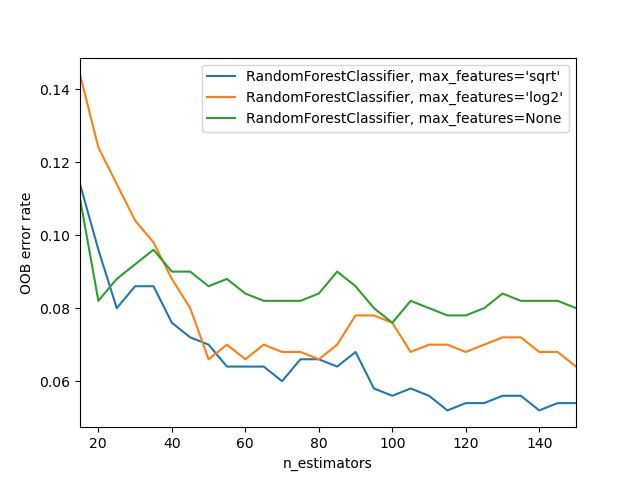"}],"metadata":{"kernelspec":{"display_name":"Python 3","language":"python","name":"python3"},"language_info":{"name":"python","version":"3.6.6","mimetype":"text/x-python","codemirror_mode":{"name":"ipython","version":3},"pygments_lexer":"ipython3","nbconvert_exporter":"python","file_extension":".py"}},"nbformat":4,"nbformat_minor":1}
\n\n[Underfitting and Overfitting](https://datascience.stackexchange.com/questions/361/when-is-a-model-underfitted)\n\n\nThe error for the pictured data points is lowest for the model on the far right (the blue curve passes through the red points almost perfectly), yet it's not the best choice. Why is that? If you were to gather some new data points, they most likely would not be on that curve in the graph on the right, but would be closer to the curve in the middle graph.\n\nThis illustrates how using all our data can lead to **overfitting**. A validation set helps diagnose this problem."},{"metadata":{"trusted":true,"_uuid":"03b0ed8a3fc084f564e39fc1e6a715b213e46968"},"cell_type":"code","source":"def split_vals(a,n): return a[:n].copy(), a[n:].copy()\n\n#Set number of rows for validation set\nn_valid = 12000 # same as Kaggle's test set size\n#Remaining number of rows is used for training set\nn_trn = len(df)-n_valid\n\n#Split unprocessed dataframe\nraw_train, raw_valid = split_vals(df_raw, n_trn)\n#Split processed dataframe and series: see proc_df() function\nX_train, X_valid = split_vals(df, n_trn)\ny_train, y_valid = split_vals(y, n_trn)\n\nX_train.shape, y_train.shape, X_valid.shape","execution_count":null,"outputs":[]},{"metadata":{"_uuid":"5d8329eaf818288f6c83d52eb3d5329e963339f3"},"cell_type":"markdown","source":"# Random Forests"},{"metadata":{"_uuid":"cf8d544aa84ddf83a24b8bef5ed75720c6f443a0"},"cell_type":"markdown","source":"## Base model"},{"metadata":{"_uuid":"2ed0cf181423696c20c92934e26e70ccdd8b265b"},"cell_type":"markdown","source":"Let's try our model again, this time with separate training and validation sets."},{"metadata":{"trusted":true,"_uuid":"f6e62979fe4dabb8fd689dbc6d42bee0c9e83fee"},"cell_type":"code","source":"def rmse(x,y): return math.sqrt(((x-y)**2).mean())\n\ndef print_score(m):\n res = [rmse(m.predict(X_train), y_train), rmse(m.predict(X_valid), y_valid),\n m.score(X_train, y_train), m.score(X_valid, y_valid)]\n if hasattr(m, 'oob_score_'): res.append(m.oob_score_)\n print(res)","execution_count":null,"outputs":[]},{"metadata":{"trusted":true,"_uuid":"5d6cfd947159d73ccfe6367fd03d9dc08fa7afbe"},"cell_type":"code","source":"m = RandomForestRegressor(n_jobs=-1)\n%time m.fit(X_train, y_train)\nprint_score(m)","execution_count":null,"outputs":[]},{"metadata":{"_uuid":"92ffd14ea998497b5947bbba7ab75b6565cb146c"},"cell_type":"markdown","source":"An r^2 in the high-80's isn't bad at all (and the RMSLE puts us around rank 100 of 470 on the Kaggle leaderboard), but we can see from the validation set score that we're over-fitting badly. To understand this issue, let's simplify things down to a single small tree."},{"metadata":{"_uuid":"c999022626c8deb82e8d7a01a3c5f9fcd2ad44b7"},"cell_type":"markdown","source":"## Speeding things up"},{"metadata":{"trusted":true,"_uuid":"dba65c173a4bf520ed2ed5ded6eba3f96e2cdc53"},"cell_type":"code","source":"df_trn, y_trn, nas = proc_df(df_raw, 'SalePrice', subset=30000, na_dict=nas)\nX_train, _ = split_vals(df_trn, 20000)\ny_train, _ = split_vals(y_trn, 20000)","execution_count":null,"outputs":[]},{"metadata":{"trusted":true,"_uuid":"bc6e18f5fd17aed0c3bb8d62c7c98ad0f4bb32da"},"cell_type":"code","source":"m = RandomForestRegressor(n_jobs=-1)\n%time m.fit(X_train, y_train)\nprint_score(m)","execution_count":null,"outputs":[]},{"metadata":{"_uuid":"4647d289cbd7cdcbd31fd5ea4d5166f4ae568235"},"cell_type":"markdown","source":"## Single tree"},{"metadata":{"trusted":true,"_uuid":"9e6d17691844ef9fa50ababd87c0eb0ca5cc492c"},"cell_type":"code","source":"# n_estimators=1: one tree\n# bootstrap=False: do not use bootstrap samples\n# \" random forest randomizes bunch of things, we want to turn that off by this parameter\"\nm = RandomForestRegressor(n_estimators=1, max_depth=3, bootstrap=False, n_jobs=-1)\nm.fit(X_train, y_train)\nprint_score(m)","execution_count":null,"outputs":[]},{"metadata":{"trusted":true,"_uuid":"284184d1414693e56b10620e22b6552de028efd4"},"cell_type":"code","source":"draw_tree(m.estimators_[0], df_trn, precision=3)","execution_count":null,"outputs":[]},{"metadata":{"_uuid":"6b6e628d571c108a71d30445c17f226b5037b33f"},"cell_type":"markdown","source":"Let's see what happens if we create a bigger tree."},{"metadata":{"trusted":true,"_uuid":"b26e645cbe05163ee4f7c28b799b82b7761e3a0d"},"cell_type":"code","source":"m = RandomForestRegressor(n_estimators=1, bootstrap=False, n_jobs=-1)\nm.fit(X_train, y_train)\nprint_score(m)","execution_count":null,"outputs":[]},{"metadata":{"_uuid":"e5d97643db5fc17d1491d523353432387140f27a"},"cell_type":"markdown","source":"The training set result looks great! But the validation set is worse than our original model. This is why we need to use *bagging* of multiple trees to get more generalizable results."},{"metadata":{"_uuid":"3aa0517b0aaebe10f38795a8d70e17cb7852b1c1"},"cell_type":"markdown","source":"## Bagging"},{"metadata":{"_uuid":"d09094ea4745e94ed20fae5e38544ed9d15db8e1"},"cell_type":"markdown","source":"### Intro to bagging"},{"metadata":{"_uuid":"68442fcd7eb5f82f8a8ec2a7ce772ac41b6a815d"},"cell_type":"markdown","source":"To learn about bagging in random forests, let's start with our basic model again."},{"metadata":{"trusted":true,"_uuid":"5af941fe1827be61fd5c0bc3d6b03abc0805dcc4"},"cell_type":"code","source":"# default number of trees is 10\nm = RandomForestRegressor(n_jobs=-1)\nm.fit(X_train, y_train)\nprint_score(m)","execution_count":null,"outputs":[]},{"metadata":{"_uuid":"3a5168a933d90491ffce0bcd10fde92baecca7d5"},"cell_type":"markdown","source":"We'll grab the predictions for each individual tree, and look at one example."},{"metadata":{"trusted":true,"_uuid":"dc6c4e1e860742bf6a56b3d58dd747f73aad612b"},"cell_type":"code","source":"# Get the predictions of each tree using the validation set\n# estimators_: List of trees\npreds = np.stack([t.predict(X_valid) for t in m.estimators_])\n\n# preds[:,0]: Predicted saleprice of each tree for first data in validation set\n# np.mean(preds[:,0]): Mean predicted saleprice (of the 10 trees)\n# y_valid[0]: Actual saleprice\npreds[:,0], np.mean(preds[:,0]), y_valid[0]","execution_count":null,"outputs":[]},{"metadata":{"trusted":true,"_uuid":"e56a9c4ff25aacae1355e5ba03a2dbb530a62946"},"cell_type":"code","source":"preds.shape","execution_count":null,"outputs":[]},{"metadata":{"trusted":true,"_uuid":"2a95bdf7abbdb7280081aaf127d93e454b001c3d"},"cell_type":"code","source":"# Plot r squared against the number of trees used (1 to 10)\n# Compare predictions against the validation set\nplt.plot([metrics.r2_score(y_valid, np.mean(preds[:i+1], axis=0)) for i in range(10)]);","execution_count":null,"outputs":[]},{"metadata":{"_uuid":"51f78a522fa6f5088e9631fd3b993e4208a54043"},"cell_type":"markdown","source":"The shape of this curve suggests that adding more trees isn't going to help us much. Let's check. (Compare this to our original model on a sample)"},{"metadata":{"trusted":true,"_uuid":"ca172db654ada609895f1db8918e5f9623e57a57"},"cell_type":"code","source":"m = RandomForestRegressor(n_estimators=20, n_jobs=-1)\nm.fit(X_train, y_train)\nprint_score(m)","execution_count":null,"outputs":[]},{"metadata":{"trusted":true,"_uuid":"02866e491723323502ce2bce12c24659a2bd5332"},"cell_type":"code","source":"m = RandomForestRegressor(n_estimators=40, n_jobs=-1)\nm.fit(X_train, y_train)\nprint_score(m)","execution_count":null,"outputs":[]},{"metadata":{"trusted":true,"_uuid":"f578620d544df3b6c26deb4e022cc99f93e6b62f"},"cell_type":"code","source":"m = RandomForestRegressor(n_estimators=80, n_jobs=-1)\nm.fit(X_train, y_train)\nprint_score(m)","execution_count":null,"outputs":[]},{"metadata":{"_uuid":"807e7f7f91ac2bbccdde1fa972d56344a3e5d345"},"cell_type":"markdown","source":"### Out-of-bag (OOB) score"},{"metadata":{"_uuid":"7ae2fb6e2bab0aef151f926427ed2db048200034"},"cell_type":"markdown","source":"Is our validation set worse than our training set because we're over-fitting, or because the validation set is for a different time period, or a bit of both? With the existing information we've shown, we can't tell. However, random forests have a very clever trick called *out-of-bag (OOB) error* which can handle this (and more!)\n\nThe idea is to calculate error on the training set, but only include the trees in the calculation of a row's error where that row was *not* included in training that tree. This allows us to see whether the model is over-fitting, without needing a separate validation set.\n\nThis also has the benefit of allowing us to see whether our model generalizes, even if we only have a small amount of data so want to avoid separating some out to create a validation set.\n\nThis is as simple as adding one more parameter to our model constructor. We print the OOB error last in our `print_score` function below."},{"metadata":{"trusted":true,"_uuid":"59f01f8b276d126b758161773bf62e43250329e4"},"cell_type":"code","source":"# oob_score=True: \"use out-of-bag samples to estimate the R^2 on unseen data\"\nm = RandomForestRegressor(n_estimators=40, n_jobs=-1, oob_score=True)\nm.fit(X_train, y_train)\nprint_score(m)","execution_count":null,"outputs":[]},{"metadata":{"_uuid":"ff6d78b33d0511ae0af00fbd7af4f21a7977ad23"},"cell_type":"markdown","source":"This shows that our validation set time difference is making an impact, as is model over-fitting."},{"metadata":{"_uuid":"6575648121f4fab7aa3b845d6405df2acead7825"},"cell_type":"markdown","source":"## Reducing over-fitting"},{"metadata":{"_uuid":"78c621c1cbdcf935d832328e666d9d7441aacb8a"},"cell_type":"markdown","source":"### Subsampling"},{"metadata":{"_uuid":"f4ab1735a914bb7ab2d3ca90d472262874cfe396"},"cell_type":"markdown","source":"It turns out that one of the easiest ways to avoid over-fitting is also one of the best ways to speed up analysis: *subsampling*. Let's return to using our full dataset, so that we can demonstrate the impact of this technique."},{"metadata":{"trusted":true,"_uuid":"4b3c4009011a8deb77167779f8b5de5e8247503f"},"cell_type":"code","source":"df_trn, y_trn, nas = proc_df(df_raw, 'SalePrice')\nX_train, X_valid = split_vals(df_trn, n_trn)\ny_train, y_valid = split_vals(y_trn, n_trn)","execution_count":null,"outputs":[]},{"metadata":{"_uuid":"b56c45f744aea566df24591f4e00f6493f6e2f56"},"cell_type":"markdown","source":"The basic idea is this: rather than limit the total amount of data that our model can access, let's instead limit it to a *different* random subset per tree. That way, given enough trees, the model can still see *all* the data, but for each individual tree it'll be just as fast as if we had cut down our dataset as before."},{"metadata":{"trusted":true,"_uuid":"f40e27536f254926ad7e51d28d60d22d9d60c81d"},"cell_type":"code","source":"set_rf_samples(20000)","execution_count":null,"outputs":[]},{"metadata":{"trusted":true,"_uuid":"4a7f184ac86f72660993574de5660fc6bf509b78"},"cell_type":"code","source":"m = RandomForestRegressor(n_jobs=-1, oob_score=True)\n%time m.fit(X_train, y_train)\nprint_score(m)","execution_count":null,"outputs":[]},{"metadata":{"_uuid":"e2696d25bb72dc352a7ad082d66f9d325273f38a"},"cell_type":"markdown","source":"Since each additional tree allows the model to see more data, this approach can make additional trees more useful."},{"metadata":{"trusted":true,"_uuid":"6f1272327940aee9875d27ca9e5125681f04a2cb"},"cell_type":"code","source":"m = RandomForestRegressor(n_estimators=40, n_jobs=-1, oob_score=True)\nm.fit(X_train, y_train)\nprint_score(m)","execution_count":null,"outputs":[]},{"metadata":{"_uuid":"8241e76e4be43018802b05ae6eeb90a252303f1b"},"cell_type":"markdown","source":"\"Question: What samples is this OOB score calculated on?\n\nScikit-learn does not support this out of box, so set_rf_samples is a custom function. So OOB score needs to be turned off when using set_rf_samples as they are not compatible. reset_rf_samples() will turn it back to the way it was.\""},{"metadata":{"_uuid":"22c04327010eb2a9107bfee538e5f12e1ffce23f"},"cell_type":"markdown","source":"### Tree building parameters"},{"metadata":{"_uuid":"0465d8d0ffa27759987d46d0d1e1db14be4afc6d"},"cell_type":"markdown","source":"We revert to using a full bootstrap sample in order to show the impact of other over-fitting avoidance methods."},{"metadata":{"trusted":true,"_uuid":"8a027d4c92012a643b69a76838f187cc4d63e950"},"cell_type":"code","source":"reset_rf_samples()","execution_count":null,"outputs":[]},{"metadata":{"_uuid":"93070592fa4b4028e348815c340872215725ff54"},"cell_type":"markdown","source":"Let's get a baseline for this full set to compare to."},{"metadata":{"trusted":true,"_uuid":"e8c9456f4d4dc11c3f03aa153bd96518e1ee24fb"},"cell_type":"code","source":"def dectree_max_depth(tree):\n children_left = tree.children_left\n children_right = tree.children_right\n\n def walk(node_id):\n if (children_left[node_id] != children_right[node_id]):\n left_max = 1 + walk(children_left[node_id])\n right_max = 1 + walk(children_right[node_id])\n return max(left_max, right_max)\n else: # leaf\n return 1\n\n root_node_id = 0\n return walk(root_node_id)","execution_count":null,"outputs":[]},{"metadata":{"trusted":true,"_uuid":"1d2bcbdb2c5670eec713c483a3ef96a77a01e7cc"},"cell_type":"code","source":"m = RandomForestRegressor(n_estimators=40, n_jobs=-1, oob_score=True)\nm.fit(X_train, y_train)\nprint_score(m)","execution_count":null,"outputs":[]},{"metadata":{"trusted":true,"_uuid":"4e86b19014d17db8c9fb7ba780f97adee8228fa4"},"cell_type":"code","source":"t=m.estimators_[0].tree_","execution_count":null,"outputs":[]},{"metadata":{"trusted":true,"_uuid":"cc0cd4abc75914f528e09e6beeeb096fbb5b46ae"},"cell_type":"code","source":"dectree_max_depth(t)","execution_count":null,"outputs":[]},{"metadata":{"trusted":true,"_uuid":"d48a8833c6bc397d6fee49c48b76cfa6045bc7bc"},"cell_type":"code","source":"# min_samples_leaf=5: \"The minimum number of samples required to be at a leaf node.\"\n# \"The numbers that work well are 1, 3, 5, 10, 25, but it is relative to your overall dataset size.\"\nm = RandomForestRegressor(n_estimators=40, min_samples_leaf=5, n_jobs=-1, oob_score=True)\nm.fit(X_train, y_train)\nprint_score(m)","execution_count":null,"outputs":[]},{"metadata":{"trusted":true,"_uuid":"e9cd3ce553fff8caa07e30199fd7952b72fe3a51"},"cell_type":"code","source":"t=m.estimators_[0].tree_","execution_count":null,"outputs":[]},{"metadata":{"trusted":true,"_uuid":"eac32886427523ee13618ef3c9a230c64fe7a58e"},"cell_type":"code","source":"dectree_max_depth(t)","execution_count":null,"outputs":[]},{"metadata":{"_uuid":"567fea0e9400b8721842a758ca27d5d7f815e99b"},"cell_type":"markdown","source":"Another way to reduce over-fitting is to grow our trees less deeply. We do this by specifying (with `min_samples_leaf`) that we require some minimum number of rows in every leaf node. This has two benefits:\n\n- There are less decision rules for each leaf node; simpler models should generalize better\n- The predictions are made by averaging more rows in the leaf node, resulting in less volatility"},{"metadata":{"trusted":true,"_uuid":"5037176ebd8869b64fa80b1f6be2df237a6b5a56"},"cell_type":"code","source":"m = RandomForestRegressor(n_estimators=40, min_samples_leaf=3, n_jobs=-1, oob_score=True)\nm.fit(X_train, y_train)\nprint_score(m)","execution_count":null,"outputs":[]},{"metadata":{"_uuid":"95c3c4113e46efa410a40f685ddfad10b584bc1e"},"cell_type":"markdown","source":"We can also increase the amount of variation amongst the trees by not only use a sample of rows for each tree, but to also using a sample of *columns* for each *split*. We do this by specifying `max_features`, which is the proportion of features to randomly select from at each split."},{"metadata":{"_uuid":"459119382bd778328d9df19b400c22beff8fe4e9"},"cell_type":"markdown","source":"- None\n- 0.5\n- 'sqrt'"},{"metadata":{"_uuid":"19c8d77d0e9e60e00c803aa6ce290fe5d24fbad2"},"cell_type":"markdown","source":"- 1, 3, 5, 10, 25, 100"},{"metadata":{"trusted":true,"_uuid":"ddd16f5c7d0699237607cb219596ad3d0202da65"},"cell_type":"code","source":"# max_features=0.5: \"The number of features to consider when looking for the best split\".\n# Consider half of all available features at each split\n# \"The idea is that the less correlated your trees are with each other, the better\"\n# \"if every tree always splits on the same thing the first time, you will not get much variation in those trees\"\n# \"Good values to use are 1, 0.5, log2, or sqrt\"\nm = RandomForestRegressor(n_estimators=40, min_samples_leaf=3, max_features=0.5, n_jobs=-1, oob_score=True)\nm.fit(X_train, y_train)\nprint_score(m)","execution_count":null,"outputs":[]},{"metadata":{"_uuid":"f65a6d2ab32c15bc9f072421f7e2768b8e57c6da"},"cell_type":"markdown","source":"We can't compare our results directly with the Kaggle competition, since it used a different validation set (and we can no longer to submit to this competition) - but we can at least see that we're getting similar results to the winners based on the dataset we have.\n\nThe sklearn docs [show an example](http://scikit-learn.org/stable/auto_examples/ensemble/plot_ensemble_oob.html) of different `max_features` methods with increasing numbers of trees - as you see, using a subset of features on each split requires using more trees, but results in better models:\n"}],"metadata":{"kernelspec":{"display_name":"Python 3","language":"python","name":"python3"},"language_info":{"name":"python","version":"3.6.6","mimetype":"text/x-python","codemirror_mode":{"name":"ipython","version":3},"pygments_lexer":"ipython3","nbconvert_exporter":"python","file_extension":".py"}},"nbformat":4,"nbformat_minor":1}