{"metadata":{"kernelspec":{"language":"python","display_name":"Python 3","name":"python3"},"language_info":{"pygments_lexer":"ipython3","nbconvert_exporter":"python","version":"3.6.4","file_extension":".py","codemirror_mode":{"name":"ipython","version":3},"name":"python","mimetype":"text/x-python"}},"nbformat_minor":4,"nbformat":4,"cells":[{"cell_type":"markdown","source":"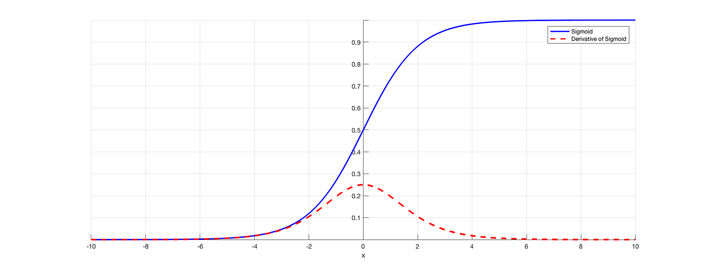 \nimg source: towards data science\n\n# Logistic regression⚙️\n\n**What you can expect from this notebook:** This is a ***follow up notebook*** to my recent one about [linear models](https://www.kaggle.com/code/vincentbrunner/ml-from-scratch-custom-linear-models), demonstrating how to turn these linear regression models into binary classification models using the logit function. \n\n
👉If you're just interested in the complete, with comments documented implementation of a logistic regression model based on a generalized form of linear models, feel free to click on show hidden code:
","metadata":{}},{"cell_type":"code","source":"import numpy as np\n\nclass Adam:\n def __init__(self, learning_rate, ß1=0.9, ß2=0.99):\n self.lr = learning_rate\n self.ß1 = ß1\n self.ß2 = ß2\n self.v = 0\n self.s = 0\n self.t = 1\n self.e = 1e-10\n \n def update_weights(self, weights, gradient):\n self.v = self.ß1 * self.v + (1 - self.ß1) * gradient\n self.s = self.ß2 * self.s + (1 - self.ß2) * gradient ** 2\n v_corrected = self.v / (1 - self.ß1 ** self.t)\n s_corrected = self.s / (1 - self.ß2 ** self.t)\n self.t += 1\n return weights - self.lr * (v_corrected / (np.sqrt(s_corrected) + self.e))\n \nclass MultivariateLogisticRegression:\n def __init__(self):\n self.feature_func_ = False\n self.weights = None\n self.sigmoid = np.vectorize(lambda x: 1 / (1 + np.exp(-x)))\n self.treshhold = 0.5\n \n def fit(self, X, y, optimizer, epochs=100, learning_rate=0.05, batch_size=64, verbose=True):\n # initialize weight vecotor\n self.weights = np.zeros(len(self.feature_func)*len(X[0])) + 1\n # initialize optimizer\n opt = optimizer(learning_rate)\n # iterate over epochs\n for e_i in range(epochs):\n # split in mini batches\n num_batches = int(np.ceil(len(X) / batch_size))\n batches = [np.array_split(X, num_batches), np.array_split(y, num_batches)]\n # iterate over batches\n for b_i in range(num_batches):\n # calculate gradient estimate\n features = np.concatenate([np.column_stack(func(batches[0][b_i])) for func in self.feature_func])\n y_pred_linear = features.T @ self.weights\n y_true = batches[1][b_i]\n gradient_point_estimates = (features * np.exp(y_pred_linear-1) * (1 - y_true)) / (np.exp(y_pred_linear-1) + 1) - (features * np.exp(-y_pred_linear) * y_true) / (np.exp(-y_pred_linear) + 1)\n gradient_mean_estimate = gradient_point_estimates.mean(axis=1)\n # weight update using optimizer\n self.weights = opt.update_weights(self.weights, gradient_mean_estimate)\n \n if verbose:\n if (e_i + 1) % 5 == 0:\n logloss = (-y * np.log(self.predict_prob(X)) - (1 - y) * np.log(1 - self.predict_prob(X) + 1e-10)).mean()\n print(f'epoch {e_i + 1}, logloss: {logloss}')\n\n def predict_prob(self, X):\n features = np.concatenate([np.column_stack(func(X)) for func in self.feature_func])\n return self.sigmoid(features.T @ self.weights)\n \n def predict(self, X):\n y_prob_pred = self.predict_prob(X)\n return np.where(y_prob_pred > self.treshhold, 1, 0)\n \n @property\n def feature_func(self):\n if type(self.feature_func_) != list:\n raise ValueError('please define the feature function before moving on')\n return self.feature_func_\n \n @feature_func.setter\n def feature_func(self, func_array): \n self.feature_func_ = [np.vectorize(func) for func in func_array]","metadata":{"execution":{"iopub.status.busy":"2022-07-31T10:27:06.644674Z","iopub.execute_input":"2022-07-31T10:27:06.645083Z","iopub.status.idle":"2022-07-31T10:27:06.670210Z","shell.execute_reply.started":"2022-07-31T10:27:06.645041Z","shell.execute_reply":"2022-07-31T10:27:06.669086Z"},"_kg_hide-input":true,"jupyter":{"source_hidden":true},"trusted":true},"execution_count":null,"outputs":[]},{"cell_type":"markdown","source":"****\n# 1 | Intuition: from regression to binary classification\n\nThe basic idea is pretty simple: Instead of directly predicting class labels, **the probability of one class is predicted**. Since binary classification is performed the probability of the other class label is just $1-p$.
\nThen **based on a threshold**, based on the predicted probability, **the output class label is determined**.\n\n**Example**:\n* y_true = **[0, 1, 1, 0, 0]**\n* predicted probabilities = **[0.2, 0.84, 0.92, 0.1, 0.4]**\n* output with a threshold of 0.5 = **[0, 1, 1, 0, 0]**\n\nProbability is a continuous quantity, so with this method, a classification task can be pseudo-transformed into a regression task. \n\n**Problem:**\nProbability is continuous only in a **closed interval from 0 to 1**. Most regression models, including most linear models discussed in the [previous notebook](https://www.kaggle.com/code/vincentbrunner/ml-from-scratch-custom-linear-models), make predictions not bounded in a specific interval. \n\n**So to use regression models to predict probabilities, the probabilities have to be transformed in a way that they range from $-\\infty$ to $+\\infty$**","metadata":{}},{"cell_type":"markdown","source":"****\n# 2 | The logit transformation\n\n \nimg source: wikipedia\n\n**The logit transformation is a way to achieve this:**\n\n$\\Large logit = log(\\frac{p}{1-p})$\n\n* The odd part of the equation($\\frac{p}{1-p}$) is the ratio of the probability of an event occurring to the probability of it not occurring\n * **it results in a quantity on a scale from 0 to $+\\infty$**\n * if the probability of the event occurring is greater than the probability of it not occurring, **the odd is greater than 1**\n * if the probability of the event occurring is less than the probability of it not occurring, **the odd is less than 1 but never less than 0**#\n \n* The logarithm takes any x between on a scale from 0 to $+\\infty$ and maps it onto a scale from $-\\infty$ to $+\\infty$\n * So by taking the logarithm of the odd equation discussed above... :\n * ... probabilities greater than 0.5 get mapped to a scale from 0 to $+\\infty$\n * ... probabilities less than 0.5 get mapped to a scale from 0 to $-\\infty$\n \n**So the goal of transforming probabilities in a way that they range from $-\\infty$ to $+\\infty$ is reached.**
\n\n### **Now the linear regression models discussed in the previous notebook can be used to predict the transformed probabilities:**\n\n$\\Large log(\\frac{p}{1-p}) = \\phi_X^T\\theta$
\n\n**By solving for p, this results in a model that directly predicts p:** \n\n$\\Large \\frac{p}{1-p} = e^{\\phi_X^T\\theta}$\n\n$\\Large p = (1-p)e^{\\phi_X^T\\theta}$\n\n$\\Large p = e^{\\phi_X^T\\theta}-pe^{\\phi_X^T\\theta}$\n\n$\\Large p + pe^{\\phi_X^T\\theta} = e^{\\phi_X^T\\theta}$\n\n$\\Large p (1 + e^{\\phi_X^T\\theta}) = e^{\\phi_X^T\\theta}$\n\n$\\Large p = \\frac{e^{\\phi_X^T\\theta}}{1 + e^{\\phi_X^T\\theta}} = \\frac{1}{1 + e^{-\\phi_X^T\\theta}}$\n\n**This results in taking the inverse of the logit, the sigmoid, of the linear model:**\n\n$\\Large \\sigma(x) = \\frac{1}{1 + e^{-x}}$\n\n \nimg source: wikipedia\n\nLooking at the sigmoid curve it's quite intuitive that it maps the unconstrained output of the model (x-axis) to an interval from 0 to 1 (y-axis).\n","metadata":{}},{"cell_type":"markdown","source":"****\n# 3 | Binary Crossentropy / Logloss\n\nTo fit the resulting Logistic Regression model, a loss function is needed, that takes predicted probabilities (p.e. [0.8, 0.1]) and corresponding labels (p.e. [1, 0]).
\n**A commonly used one is the binary cross-entropy aka. log loss aka. negative log-likelihood:**\n\n$\\Large logloss = -\\frac{1}{n}\\sum\\limits_{i=1}^nplog(\\hat{p})+(1-p)log(1-\\hat{p})$\n\nWhen assuming the labels (in this case p) to be just 0 or 1 this formula just boils down to:\n\n$\\Large log loss = -\\frac{1}{n}\\sum\\limits_{i=1}^n \\left\\{ \\begin{array}{ c l }log(\\hat{p}) & \\quad \\textrm{if } p = 1 \\\\ log(1-\\hat{p}) & \\quad \\textrm{if } p = 0 \\end{array}\\right.$\n\nThis is done cause every prediction is the probability for the label to be 1. So by taking 1 - the predicted probability, the probability for event 0 occurring is obtained.
\n**So the log loss takes the negative log of the predicted probability for the corresponding target event to occur and averages the results.**\n\n \nimg source: ljvmiranda921.github.io\n\nSo the loss is higher the further away the predicted probability for the corresponding target event to occur is from 1. ","metadata":{}},{"cell_type":"markdown","source":"****\n# 4 | Python implementation\n\n* With that background knowledge the code for the linear models from the [previous notebook](https://www.kaggle.com/code/vincentbrunner/ml-from-scratch-custom-linear-models) can be modified to apply the sigmoid function to its output.\n* Additionally the **Adam optimizer** is implemented to fit the model using the log loss discussed above.","metadata":{}},{"cell_type":"code","source":"import numpy as np # linear algebra\nimport pandas as pd # data handeling\nfrom sklearn.model_selection import train_test_split # splitting data in train/test set\nimport seaborn as sns # data visualisation\nimport matplotlib.pyplot as plt # data visualisation\nfrom sklearn.metrics import confusion_matrix, ConfusionMatrixDisplay # creating & visualising confusion matrices\nfrom sklearn.model_selection import train_test_split # splitting data in train/test set","metadata":{"execution":{"iopub.status.busy":"2022-08-01T09:21:16.441008Z","iopub.execute_input":"2022-08-01T09:21:16.441538Z","iopub.status.idle":"2022-08-01T09:21:17.402796Z","shell.execute_reply.started":"2022-08-01T09:21:16.441423Z","shell.execute_reply":"2022-08-01T09:21:17.401296Z"},"trusted":true},"execution_count":null,"outputs":[]},{"cell_type":"markdown","source":"**gradient descent:** I explained this iterative way of optimizing an objective function in detail here: [ml from scratch: neural network and GD-optimizers](https://www.kaggle.com/code/vincentbrunner/ml-from-scratch-neural-network-and-gd-optimizers)
\nThe implementation below allows for any gradient-based optimizer, but in the **mini-batch gradient descent** fashion.\n\nThe gradient of the logistic regression model (sigmoid of a linear model) over its parameters is just:\n\n$\\huge \\frac{\\phi_Xe^{\\hat{y} - 1}(1-y)}{e^{\\hat{y} - 1} + 1} - \\frac{\\phi_Xe^{-\\hat{y}}y}{e^{-\\hat{y}} + 1}$","metadata":{}},{"cell_type":"code","source":"class MultivariateLogisticRegression:\n def __init__(self):\n self.feature_func_ = False\n self.weights = None\n # sigmoid function\n self.sigmoid = np.vectorize(lambda x: 1 / (1 + np.exp(-x)))\n # treshold to predict binary labels based on predicted probabilities -> see 1|intuition\n self.treshhold = 0.5\n \n def fit(self, X, y, optimizer, epochs=100, learning_rate=0.05, batch_size=64, verbose=True):\n # initialize weight vecotor\n self.weights = np.zeros(len(self.feature_func)*len(X[0])) + 1\n # initialize optimizer\n opt = optimizer(learning_rate)\n # iterate over epochs\n for e_i in range(epochs):\n # split in mini batches\n num_batches = int(np.ceil(len(X) / batch_size))\n batches = [np.array_split(X, num_batches), np.array_split(y, num_batches)]\n # iterate over batches\n for b_i in range(num_batches):\n # calculate gradient estimate\n features = np.concatenate([np.column_stack(func(batches[0][b_i])) for func in self.feature_func])\n y_pred_linear = features.T @ self.weights\n y_true = batches[1][b_i]\n gradient_point_estimates = (features * np.exp(y_pred_linear-1) * (1 - y_true)) / (np.exp(y_pred_linear-1) + 1) - (features * np.exp(-y_pred_linear) * y_true) / (np.exp(-y_pred_linear) + 1)\n gradient_mean_estimate = gradient_point_estimates.mean(axis=1)\n # weight update using optimizer\n self.weights = opt.update_weights(self.weights, gradient_mean_estimate)\n \n if verbose:\n if (e_i + 1) % 5 == 0:\n logloss = (-y * np.log(self.predict_prob(X)) - (1 - y) * np.log(1 - self.predict_prob(X) + 1e-10)).mean()\n print(f'epoch {e_i + 1}, logloss: {logloss}')\n \n # makes predictions of linear model and passes through sigmoid to obtain probabilies\n def predict_prob(self, X):\n features = np.concatenate([np.column_stack(func(X)) for func in self.feature_func])\n return self.sigmoid(features.T @ self.weights)\n \n # uses treshold to turn predicted probabilities into binary targets (0 or 1)\n def predict(self, X):\n y_prob_pred = self.predict_prob(X)\n return np.where(y_prob_pred > self.treshhold, 1, 0)\n \n # using a property to deal with the assignment of the feature function\n @property\n def feature_func(self):\n # checking if the feature function is allready set\n if type(self.feature_func_) != list:\n raise ValueError('please define the feature function before moving on')\n return self.feature_func_\n \n @feature_func.setter\n def feature_func(self, func_array): \n # np.vectorize allows to pass a numpy array trough the function\n self.feature_func_ = [np.vectorize(func) for func in func_array]","metadata":{"execution":{"iopub.status.busy":"2022-08-01T09:37:36.743040Z","iopub.execute_input":"2022-08-01T09:37:36.743459Z","iopub.status.idle":"2022-08-01T09:37:36.765863Z","shell.execute_reply.started":"2022-08-01T09:37:36.743427Z","shell.execute_reply":"2022-08-01T09:37:36.764115Z"},"trusted":true},"execution_count":null,"outputs":[]},{"cell_type":"markdown","source":"**Adam** is a gradient descent based optimizer I explained here: [ml from scratch: neural network and GD-optimizers](https://www.kaggle.com/code/vincentbrunner/ml-from-scratch-neural-network-and-gd-optimizers). It's a bit overkill for this optimization problem, but I had fun playing around with the implementation a bit.","metadata":{}},{"cell_type":"code","source":"class Adam:\n def __init__(self, learning_rate, ß1=0.9, ß2=0.99):\n self.lr = learning_rate\n self.ß1 = ß1\n self.ß2 = ß2\n self.v = 0\n self.s = 0\n self.t = 1\n self.e = 1e-10\n \n def update_weights(self, weights, gradient):\n # exp. moving average term for gradient -> 'momentum buffer'\n self.v = self.ß1 * self.v + (1 - self.ß1) * gradient\n # exp. moving average term for squared gradient -> addaptive learning rate\n self.s = self.ß2 * self.s + (1 - self.ß2) * gradient ** 2\n # bias correction for both terms\n v_corrected = self.v / (1 - self.ß1 ** self.t)\n s_corrected = self.s / (1 - self.ß2 ** self.t)\n self.t += 1\n # final weight update\n return weights - self.lr * (v_corrected / (np.sqrt(s_corrected) + self.e))","metadata":{"execution":{"iopub.status.busy":"2022-08-01T09:46:23.037005Z","iopub.execute_input":"2022-08-01T09:46:23.037466Z","iopub.status.idle":"2022-08-01T09:46:23.049959Z","shell.execute_reply.started":"2022-08-01T09:46:23.037430Z","shell.execute_reply":"2022-08-01T09:46:23.048570Z"},"trusted":true},"execution_count":null,"outputs":[]},{"cell_type":"markdown","source":"****\n# 5 | Fitting and evaluation","metadata":{}},{"cell_type":"code","source":"titanic_data = pd.read_csv(\"../input/titanic/train.csv\", usecols=[\"Survived\", \"Sex\", \"Age\", \"SibSp\", \"Parch\", \"Fare\", \"Embarked\"]).dropna()\ntitanic_data[\"Sex\"] = titanic_data[\"Sex\"].astype(\"category\").cat.codes\ntitanic_data[\"Embarked\"] = titanic_data[\"Embarked\"].astype(\"category\").cat.codes\n\nfeatures = titanic_data.loc[:, titanic_data.columns!=\"Survived\"].to_numpy() # select everything but the target\nlabels = titanic_data.loc[:, \"Survived\"].to_numpy() # select the target\n\nX_train, X_val, y_train, y_val = train_test_split(features, labels, test_size=0.2)\n\ntitanic_data.head()","metadata":{"execution":{"iopub.status.busy":"2022-08-01T09:46:26.042176Z","iopub.execute_input":"2022-08-01T09:46:26.042588Z","iopub.status.idle":"2022-08-01T09:46:26.111816Z","shell.execute_reply.started":"2022-08-01T09:46:26.042555Z","shell.execute_reply":"2022-08-01T09:46:26.110344Z"},"trusted":true},"execution_count":null,"outputs":[]},{"cell_type":"markdown","source":"#### **Let's first fit a Logistic Regression model based on a simple line:**","metadata":{}},{"cell_type":"code","source":"lm = MultivariateLogisticRegression()\nlm.feature_func = [lambda x: 1, lambda x: x]\n\nlm.fit(X_train, y_train, Adam)","metadata":{"execution":{"iopub.status.busy":"2022-08-01T09:47:55.491427Z","iopub.execute_input":"2022-08-01T09:47:55.491839Z","iopub.status.idle":"2022-08-01T09:47:56.444599Z","shell.execute_reply.started":"2022-08-01T09:47:55.491805Z","shell.execute_reply":"2022-08-01T09:47:56.443337Z"},"trusted":true},"execution_count":null,"outputs":[]},{"cell_type":"code","source":"predictions = lm.predict(X_val)\n\n# confusion matrix\ncm = confusion_matrix(y_val, predictions, labels=[0, 1])\ncm_displ = ConfusionMatrixDisplay(cm)\ncm_displ.plot()\nplt.show()\n\n# calculate accuracy:\naccuracy = np.mean(predictions==y_val)\n\n# calculate recall:\nrecall = cm[1, 1]/cm[1, :].sum() # of the total actual positives, how much were classified correctly\n\n# calculate precision:\nprecision = cm[1, 1]/cm[:, 1].sum() # of all predicted positives, how much were True positives\n\n# not that neccessary for this problem, but for the completeness:\nf1 = 2 * ((recall * precision)/(recall + precision)) \n\nprint(f\"accuracy = {accuracy},\\nrecall = {recall},\\nprecision = {precision},\\nf1-score = {f1}\")","metadata":{"execution":{"iopub.status.busy":"2022-08-01T09:48:06.747109Z","iopub.execute_input":"2022-08-01T09:48:06.748138Z","iopub.status.idle":"2022-08-01T09:48:07.034366Z","shell.execute_reply.started":"2022-08-01T09:48:06.748097Z","shell.execute_reply":"2022-08-01T09:48:07.032884Z"},"trusted":true},"execution_count":null,"outputs":[]},{"cell_type":"markdown","source":"#### **But this also works with any other linear model, p.e. a combination of gaußian features:**","metadata":{}},{"cell_type":"code","source":"gaußian = lambda x, c: np.exp(-(x - c) ** 2/2)\nlm.feature_func = [lambda x: gaußian(x, 2), lambda x: gaußian(x, 4), lambda x: gaußian(x, 6), lambda x: x, lambda x: 1]\n\nlm.fit(X_train, y_train, Adam)","metadata":{"execution":{"iopub.status.busy":"2022-08-01T09:49:11.779258Z","iopub.execute_input":"2022-08-01T09:49:11.779732Z","iopub.status.idle":"2022-08-01T09:49:18.300500Z","shell.execute_reply.started":"2022-08-01T09:49:11.779696Z","shell.execute_reply":"2022-08-01T09:49:18.298846Z"},"trusted":true},"execution_count":null,"outputs":[]},{"cell_type":"code","source":"predictions = lm.predict(X_val)\n\n# confusion matrix\ncm = confusion_matrix(y_val, predictions, labels=[0, 1])\ncm_displ = ConfusionMatrixDisplay(cm)\ncm_displ.plot()\nplt.show()\n\n# calculate accuracy:\naccuracy = np.mean(predictions==y_val)\n\n# calculate recall:\nrecall = cm[1, 1]/cm[1, :].sum() # of the total actual positives, how much were classified correctly\n\n# calculate precision:\nprecision = cm[1, 1]/cm[:, 1].sum() # of all predicted positives, how much were True positives\n\n# not that neccessary for this problem, but for the completeness:\nf1 = 2 * ((recall * precision)/(recall + precision)) \n\nprint(f\"accuracy = {accuracy},\\nrecall = {recall},\\nprecision = {precision},\\nf1-score = {f1}\")","metadata":{"execution":{"iopub.status.busy":"2022-08-01T09:49:21.744618Z","iopub.execute_input":"2022-08-01T09:49:21.745033Z","iopub.status.idle":"2022-08-01T09:49:22.005314Z","shell.execute_reply.started":"2022-08-01T09:49:21.745000Z","shell.execute_reply":"2022-08-01T09:49:22.004177Z"},"trusted":true},"execution_count":null,"outputs":[]},{"cell_type":"markdown","source":"This is a simple way to add complexity to a logistic regression model.","metadata":{}},{"cell_type":"markdown","source":"**That's all for this notebook, have a great day and happy learning!👋**","metadata":{}}]}