\n\n ","metadata":{}},{"cell_type":"markdown","source":"
\n
Markdown(Comment cell) and Code cell
\n","metadata":{}},{"cell_type":"markdown","source":"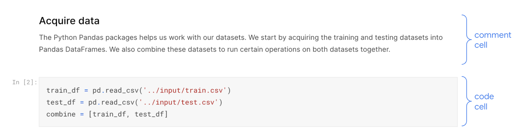","metadata":{}},{"cell_type":"code","source":"import pandas as pd\nimport numpy as np\nimport time\nfrom tqdm import tqdm\nimport gc\ngc.collect()\n\n\nfrom wordcloud import WordCloud, STOPWORDS, ImageColorGenerator\nfrom sklearn.feature_extraction.text import CountVectorizer\n\nfrom PIL import Image\nfrom nltk.corpus import stopwords\nstop=set(stopwords.words('english'))\nfrom nltk.util import ngrams\n\n\nimport re\nfrom collections import Counter\n\nimport nltk\nfrom nltk.corpus import stopwords\n\nimport warnings\nwarnings.filterwarnings(\"ignore\")\n\nimport matplotlib.pyplot as plt\nimport plotly.express as px\nimport plotly.graph_objects as go\nimport plotly.figure_factory as ff\nfrom plotly.colors import n_colors\nfrom plotly.subplots import make_subplots","metadata":{"execution":{"iopub.status.busy":"2022-05-12T19:40:27.569753Z","iopub.execute_input":"2022-05-12T19:40:27.570476Z","iopub.status.idle":"2022-05-12T19:40:31.816463Z","shell.execute_reply.started":"2022-05-12T19:40:27.570332Z","shell.execute_reply":"2022-05-12T19:40:31.81575Z"},"trusted":true},"execution_count":null,"outputs":[]},{"cell_type":"markdown","source":"
\n
In this notebook for the EDA Purposes, we will using the dataset by Darien Schettler - https://www.kaggle.com/dschettler8845
\n Dataset Link - https://www.kaggle.com/datasets/dschettler8845/ai4code-train-dataframe/
\n\n","metadata":{"execution":{"iopub.status.busy":"2022-05-12T16:55:27.189317Z","iopub.execute_input":"2022-05-12T16:55:27.189721Z","iopub.status.idle":"2022-05-12T16:55:27.197295Z","shell.execute_reply.started":"2022-05-12T16:55:27.189682Z","shell.execute_reply":"2022-05-12T16:55:27.19628Z"}}},{"cell_type":"code","source":"train_data=pd.read_csv('../input/ai4code-train-dataframe/train.csv')\n#train_data.drop(columns=['Unnamed: 0'],inplace=True)\nprint('Number of records in the train data:',train_data.shape)\nprint('Number of Notebooks:',train_data['id'].nunique())\nprint('Number of different cell types:',train_data['cell_type'].nunique(),'(Code and Markdown cell)')\n\ngc.collect()","metadata":{"execution":{"iopub.status.busy":"2022-05-12T19:40:31.818294Z","iopub.execute_input":"2022-05-12T19:40:31.819044Z","iopub.status.idle":"2022-05-12T19:41:28.398747Z","shell.execute_reply.started":"2022-05-12T19:40:31.818992Z","shell.execute_reply":"2022-05-12T19:41:28.39779Z"},"trusted":true},"execution_count":null,"outputs":[]},{"cell_type":"code","source":"train_data.info(memory_usage='deep')","metadata":{"execution":{"iopub.status.busy":"2022-05-12T19:41:28.400159Z","iopub.execute_input":"2022-05-12T19:41:28.400431Z","iopub.status.idle":"2022-05-12T19:41:31.219337Z","shell.execute_reply.started":"2022-05-12T19:41:28.400396Z","shell.execute_reply":"2022-05-12T19:41:31.218379Z"},"trusted":true},"execution_count":null,"outputs":[]},{"cell_type":"code","source":"train_data.head()","metadata":{"execution":{"iopub.status.busy":"2022-05-12T19:41:31.221852Z","iopub.execute_input":"2022-05-12T19:41:31.222791Z","iopub.status.idle":"2022-05-12T19:41:31.240576Z","shell.execute_reply.started":"2022-05-12T19:41:31.222751Z","shell.execute_reply":"2022-05-12T19:41:31.239652Z"},"trusted":true},"execution_count":null,"outputs":[]},{"cell_type":"code","source":"print('Number of records in the train data:',train_data.shape)\nprint('Number of Notebooks:',train_data['id'].nunique())\nprint('Number of different cell types:',train_data['cell_type'].nunique(),'(Code and Markdown cell)')\n","metadata":{"execution":{"iopub.status.busy":"2022-05-12T19:41:31.241894Z","iopub.execute_input":"2022-05-12T19:41:31.242453Z","iopub.status.idle":"2022-05-12T19:41:32.060416Z","shell.execute_reply.started":"2022-05-12T19:41:31.242413Z","shell.execute_reply":"2022-05-12T19:41:32.059458Z"},"trusted":true},"execution_count":null,"outputs":[]},{"cell_type":"code","source":"import seaborn as sns\nimport matplotlib.pyplot as plt\n%matplotlib inline \nsns.set(rc={'figure.figsize':(10,6)})\ncustom_colors = [\"#4e89ae\", \"#c56183\",\"#ed6663\",\"#ffa372\"]\n\ndef triple_plot(x, title,c): # Use trtrain_datae plot for numeric and important key features \n fig, ax = plt.subplots(3,1,figsize=(20,10),sharex=True)\n sns.distplot(x, ax=ax[0],color=c)\n ax[0].set(xlabel=None)\n ax[0].set_title('Histogram + KDE')\n sns.boxplot(x, ax=ax[1],color=c)\n ax[1].set(xlabel=None)\n ax[1].set_title('Boxplot')\n sns.violinplot(x, ax=ax[2],color=c)\n ax[2].set(xlabel=None)\n ax[2].set_title('Violin plot')\n #fig.suptitle(title, fontsize=30)\n #plt.tight_layout(pad=3.0)\n plt.show();\n\n#Aggregating by notebook ids to get the count\ncounter=pd.DataFrame(train_data.groupby(['id']).agg({'cell_id':'count','cell_type':'nunique'}))\ncounter.rename(columns={'cell_id':'Cell_count'},inplace=True)\ncounter=counter[counter['Cell_count']!=0]\n\ntriple_plot(counter['Cell_count'],'Distribution of cells in Notebooks',custom_colors[2])","metadata":{"execution":{"iopub.status.busy":"2022-05-12T19:41:32.061713Z","iopub.execute_input":"2022-05-12T19:41:32.061956Z","iopub.status.idle":"2022-05-12T19:41:36.024614Z","shell.execute_reply.started":"2022-05-12T19:41:32.061926Z","shell.execute_reply":"2022-05-12T19:41:36.023676Z"},"trusted":true},"execution_count":null,"outputs":[]},{"cell_type":"markdown","source":"
\n\n
The above graph shows us the distribution of number of cells present in each and every notebook that is present in the training dataset
\nAs you can see, the above distribution is skewed(Log normal distribution), at this point it would be ideal to use median as a central tendency measure rather than using mean
\nWe also see outliers in the above graph, bu the violin chart shows us that the distribution is very less
\n","metadata":{}},{"cell_type":"code","source":"print('Median number of cells in the notebooks:',counter['Cell_count'].median())","metadata":{"execution":{"iopub.status.busy":"2022-05-12T19:41:36.025959Z","iopub.execute_input":"2022-05-12T19:41:36.026196Z","iopub.status.idle":"2022-05-12T19:41:36.035434Z","shell.execute_reply.started":"2022-05-12T19:41:36.026166Z","shell.execute_reply":"2022-05-12T19:41:36.03427Z"},"trusted":true},"execution_count":null,"outputs":[]},{"cell_type":"code","source":"counter.describe()","metadata":{"execution":{"iopub.status.busy":"2022-05-12T19:41:36.036992Z","iopub.execute_input":"2022-05-12T19:41:36.037224Z","iopub.status.idle":"2022-05-12T19:41:36.063878Z","shell.execute_reply.started":"2022-05-12T19:41:36.037195Z","shell.execute_reply":"2022-05-12T19:41:36.06303Z"},"trusted":true},"execution_count":null,"outputs":[]},{"cell_type":"markdown","source":"
\n\n
Obviously, there are only two cell types - Code cell and mardown cell
\nAs you can see, Nearly 75% of the data points(Notebooks) have a cell count of 57 and 50% of the data points have a cell count of 35
\n ","metadata":{}},{"cell_type":"markdown","source":"
\n
Let's look at the training examples
\n","metadata":{}},{"cell_type":"code","source":"# I have just shown the cells for one single notebook (8a2564b730a575)\ntrain_data[train_data['id']=='8a2564b730a575']","metadata":{"execution":{"iopub.status.busy":"2022-05-12T19:41:36.065043Z","iopub.execute_input":"2022-05-12T19:41:36.065709Z","iopub.status.idle":"2022-05-12T19:41:36.492229Z","shell.execute_reply.started":"2022-05-12T19:41:36.065678Z","shell.execute_reply":"2022-05-12T19:41:36.491303Z"},"trusted":true},"execution_count":null,"outputs":[]},{"cell_type":"markdown","source":"
\n
Let's look at an another example as similiar to the above one but just in elaborate manner
\n","metadata":{}},{"cell_type":"code","source":"[print('\\033[1m'+'This is Cell {}:\\n \\t\\n'.format(j+1)+'\\033[0m'+str(i) + '\\n'+'---------------------------------------------------------\\n\\n')for j,i in enumerate(train_data[train_data['id']==train_data['id'].iloc[2]]['source'])]","metadata":{"execution":{"iopub.status.busy":"2022-05-12T19:41:36.495834Z","iopub.execute_input":"2022-05-12T19:41:36.496128Z","iopub.status.idle":"2022-05-12T19:41:36.906141Z","shell.execute_reply.started":"2022-05-12T19:41:36.496092Z","shell.execute_reply":"2022-05-12T19:41:36.905433Z"},"trusted":true},"execution_count":null,"outputs":[]},{"cell_type":"markdown","source":"
\n\n
Please Note:
\n\nThe code cells are in their original (correct) order. The markdown cell(Cell 12 above) has been shuffled and placed after the code cells.
\n\nYour task is to predict the correct ordering of the markdown cell in a given notebook as they are shuffled.
\n","metadata":{}},{"cell_type":"markdown","source":"
\n\n
Binning the cell count
\n\nIn order for better interpretation, I have binned the cell counts of notebooks into five different categories
\n\n
\n \n* Very small Notebook - 0 to 10 cells\n* Small notebook - 11 to 20 cells\n* Medium Notebooks - 21 to 50 cells\n* Large Notebooks - 51 to 100 cells\n* Very large notebooks - >100 cells \n\n You can always change the numbers according to your need in the cell_binner list down below
\n","metadata":{}},{"cell_type":"code","source":"#Binning conditions\ncell_binner=[0,10,20,50,100,99999]\nlabels=['Very Small NB','Small NB','Medium NB','Large NB','Very Large NB']\n\n#Lets bin the cell count into five different categories as explained above \ncounter['cells_bin']=pd.cut(counter['Cell_count'],bins=cell_binner,labels=labels)\n\n#Also merge the binned results with the train data\ntrain_data=train_data.merge(counter.reset_index()[['id','cells_bin']],on=['id'],how='left')\n\n#Distribution calculation of the bins \nnb_split=pd.DataFrame(counter['cells_bin'].value_counts()).reset_index()\nnb_split.columns=['Category','Number of NBs']\nnb_split['Percentage(%)']=round(((nb_split['Number of NBs']/nb_split['Number of NBs'].sum())*100),2)\nnb_split","metadata":{"execution":{"iopub.status.busy":"2022-05-12T19:41:36.907717Z","iopub.execute_input":"2022-05-12T19:41:36.908458Z","iopub.status.idle":"2022-05-12T19:41:38.481969Z","shell.execute_reply.started":"2022-05-12T19:41:36.908408Z","shell.execute_reply":"2022-05-12T19:41:38.480674Z"},"trusted":true},"execution_count":null,"outputs":[]},{"cell_type":"markdown","source":"
\n
Nearly 44% of the notebooks come under the medium category(21-50 cells) followed by Large notebboks, which is around 23%
\n","metadata":{"execution":{"iopub.status.busy":"2022-05-12T16:58:52.105846Z","iopub.execute_input":"2022-05-12T16:58:52.106378Z","iopub.status.idle":"2022-05-12T16:58:52.124858Z","shell.execute_reply.started":"2022-05-12T16:58:52.106329Z","shell.execute_reply":"2022-05-12T16:58:52.124185Z"}}},{"cell_type":"code","source":"def build_wordcloud(df, title):\n wordcloud = WordCloud(\n background_color='black',colormap=\"Oranges\", \n stopwords=set(STOPWORDS), \n max_words=50, \n max_font_size=40, \n random_state=666\n ).generate(str(df))\n\n fig = plt.figure(1, figsize=(14,14))\n plt.axis('off')\n fig.suptitle(title, fontsize=16)\n fig.subplots_adjust(top=2.3)\n\n plt.imshow(wordcloud)\n plt.show()\n \n","metadata":{"execution":{"iopub.status.busy":"2022-05-12T19:41:38.483463Z","iopub.execute_input":"2022-05-12T19:41:38.484365Z","iopub.status.idle":"2022-05-12T19:41:38.492558Z","shell.execute_reply.started":"2022-05-12T19:41:38.484316Z","shell.execute_reply":"2022-05-12T19:41:38.491557Z"},"trusted":true},"execution_count":null,"outputs":[]},{"cell_type":"markdown","source":"
\n
Lets see the Word Cloud for different categories
\n","metadata":{}},{"cell_type":"code","source":"build_wordcloud(train_data['source'], 'Prevalent words in all the Notebooks')","metadata":{"execution":{"iopub.status.busy":"2022-05-12T19:41:38.494323Z","iopub.execute_input":"2022-05-12T19:41:38.49516Z","iopub.status.idle":"2022-05-12T19:41:38.839461Z","shell.execute_reply.started":"2022-05-12T19:41:38.495122Z","shell.execute_reply":"2022-05-12T19:41:38.838566Z"},"trusted":true},"execution_count":null,"outputs":[]},{"cell_type":"code","source":"build_wordcloud(train_data[train_data['cells_bin']=='Small NB']['source'], 'Prevalent words in all the Small Notebooks')","metadata":{"execution":{"iopub.status.busy":"2022-05-12T19:41:38.840937Z","iopub.execute_input":"2022-05-12T19:41:38.841714Z","iopub.status.idle":"2022-05-12T19:41:39.230496Z","shell.execute_reply.started":"2022-05-12T19:41:38.841651Z","shell.execute_reply":"2022-05-12T19:41:39.229673Z"},"trusted":true},"execution_count":null,"outputs":[]},{"cell_type":"code","source":"build_wordcloud(train_data[train_data['cells_bin']=='Very Small NB']['source'], 'Prevalent words in all the Very Small Notebooks')","metadata":{"execution":{"iopub.status.busy":"2022-05-12T19:41:39.232214Z","iopub.execute_input":"2022-05-12T19:41:39.232879Z","iopub.status.idle":"2022-05-12T19:41:39.543592Z","shell.execute_reply.started":"2022-05-12T19:41:39.232831Z","shell.execute_reply":"2022-05-12T19:41:39.542762Z"},"trusted":true},"execution_count":null,"outputs":[]},{"cell_type":"code","source":"build_wordcloud(train_data[train_data['cells_bin']=='Medium NB']['source'], 'Prevalent words in all the Medium Notebooks')","metadata":{"execution":{"iopub.status.busy":"2022-05-12T19:41:39.54524Z","iopub.execute_input":"2022-05-12T19:41:39.545522Z","iopub.status.idle":"2022-05-12T19:41:40.23098Z","shell.execute_reply.started":"2022-05-12T19:41:39.545487Z","shell.execute_reply":"2022-05-12T19:41:40.229855Z"},"trusted":true},"execution_count":null,"outputs":[]},{"cell_type":"code","source":"build_wordcloud(train_data[train_data['cells_bin']=='High NB']['source'], 'Prevalent words in all the higher number of cells (50-100) Notebook')","metadata":{"execution":{"iopub.status.busy":"2022-05-12T19:41:40.232763Z","iopub.execute_input":"2022-05-12T19:41:40.233067Z","iopub.status.idle":"2022-05-12T19:41:40.447322Z","shell.execute_reply.started":"2022-05-12T19:41:40.233023Z","shell.execute_reply":"2022-05-12T19:41:40.446281Z"},"trusted":true},"execution_count":null,"outputs":[]},{"cell_type":"code","source":"build_wordcloud(train_data[train_data['cells_bin']=='Very High NB']['source'], 'Prevalent words in all the very higher number of cells (>100 cells) notebook')","metadata":{"execution":{"iopub.status.busy":"2022-05-12T19:41:40.449081Z","iopub.execute_input":"2022-05-12T19:41:40.449395Z","iopub.status.idle":"2022-05-12T19:41:40.719631Z","shell.execute_reply.started":"2022-05-12T19:41:40.449351Z","shell.execute_reply":"2022-05-12T19:41:40.718358Z"},"trusted":true},"execution_count":null,"outputs":[]},{"cell_type":"code","source":"build_wordcloud(train_data[train_data['cell_type']=='code']['source'], 'Prevalent words in all the CODE cells')","metadata":{"execution":{"iopub.status.busy":"2022-05-12T19:41:40.721278Z","iopub.execute_input":"2022-05-12T19:41:40.7216Z","iopub.status.idle":"2022-05-12T19:41:42.126354Z","shell.execute_reply.started":"2022-05-12T19:41:40.721546Z","shell.execute_reply":"2022-05-12T19:41:42.125194Z"},"trusted":true},"execution_count":null,"outputs":[]},{"cell_type":"code","source":"build_wordcloud(train_data[train_data['cell_type']=='markdown']['source'], 'Prevalent words in all the Markdown cells')","metadata":{"execution":{"iopub.status.busy":"2022-05-12T19:41:42.127826Z","iopub.execute_input":"2022-05-12T19:41:42.128179Z","iopub.status.idle":"2022-05-12T19:41:43.169744Z","shell.execute_reply.started":"2022-05-12T19:41:42.12814Z","shell.execute_reply":"2022-05-12T19:41:43.16869Z"},"trusted":true},"execution_count":null,"outputs":[]},{"cell_type":"code","source":"%%time\ntrain_data['text_length']=train_data['source'].apply(lambda x: len(str(x).split()))","metadata":{"execution":{"iopub.status.busy":"2022-05-12T19:45:35.722604Z","iopub.execute_input":"2022-05-12T19:45:35.72336Z","iopub.status.idle":"2022-05-12T19:45:50.168824Z","shell.execute_reply.started":"2022-05-12T19:45:35.723299Z","shell.execute_reply":"2022-05-12T19:45:50.167766Z"},"trusted":true},"execution_count":null,"outputs":[]},{"cell_type":"markdown","source":"
\n
Let's observe the text length in markdowns
\n ","metadata":{}},{"cell_type":"code","source":"triple_plot(train_data[(train_data['cell_type']=='markdown')]['text_length'],'Distribution of text length in markdowns',custom_colors[2])","metadata":{"execution":{"iopub.status.busy":"2022-05-12T19:45:56.425798Z","iopub.execute_input":"2022-05-12T19:45:56.426279Z","iopub.status.idle":"2022-05-12T19:46:08.82977Z","shell.execute_reply.started":"2022-05-12T19:45:56.426245Z","shell.execute_reply":"2022-05-12T19:46:08.828586Z"},"trusted":true},"execution_count":null,"outputs":[]},{"cell_type":"markdown","source":"
\n
Due to the extreme outliers, it s hard to interpret any inference so using IQR, we can follow the below approach to replace the outliers with a NULL value:
\n
\n \n* Calculate the first and third quartile (Q1 and Q3).\n* Further, evaluate the interquartile range, IQR = Q3-Q1.\n* Estimate the lower bound, the lower bound = Q1*1.5\n* Estimate the upper bound, upper bound = Q3*1.5\n* Replace the data points that lie outside of the lower and the upper bound with a NULL value\n\n","metadata":{}},{"cell_type":"code","source":"for x in ['text_length']:\n q75,q25 = np.percentile(train_data.loc[:,x],[75,25])\n intr_qr = q75-q25\n \n max = q75+(1.5*intr_qr)\n min = q25-(1.5*intr_qr)\n \n train_data.loc[train_data[x] < min,x] = np.nan\n train_data.loc[train_data[x] > max,x] = np.nan","metadata":{"execution":{"iopub.status.busy":"2022-05-12T19:47:23.995727Z","iopub.execute_input":"2022-05-12T19:47:23.996371Z","iopub.status.idle":"2022-05-12T19:47:24.283638Z","shell.execute_reply.started":"2022-05-12T19:47:23.996323Z","shell.execute_reply":"2022-05-12T19:47:24.28279Z"},"trusted":true},"execution_count":null,"outputs":[]},{"cell_type":"code","source":"triple_plot(train_data[(train_data['cell_type']=='markdown')]['text_length'],'Distribution of text length in markdowns',custom_colors[2])","metadata":{"execution":{"iopub.status.busy":"2022-05-12T19:47:26.669072Z","iopub.execute_input":"2022-05-12T19:47:26.669401Z","iopub.status.idle":"2022-05-12T19:47:39.241959Z","shell.execute_reply.started":"2022-05-12T19:47:26.669363Z","shell.execute_reply":"2022-05-12T19:47:39.241209Z"},"trusted":true},"execution_count":null,"outputs":[]},{"cell_type":"markdown","source":"
\n
N-GRAM
\n
Listing below the top N-gram sequential words used in Markdown cells
\n\n\n","metadata":{}},{"cell_type":"code","source":"%%time\ndef ngram_df(corpus,nrange,n=None):\n vec = CountVectorizer(stop_words = 'english',ngram_range=nrange).fit(corpus)\n bag_of_words = vec.transform(corpus)\n sum_words = bag_of_words.sum(axis=0) \n words_freq = [(word, sum_words[0, idx]) for word, idx in vec.vocabulary_.items()]\n words_freq =sorted(words_freq, key = lambda x: x[1], reverse=True)\n total_list=words_freq[:n]\n df=pd.DataFrame(total_list,columns=['text','count'])\n return df\nunigram_df=ngram_df(train_data[(train_data['cell_type']=='markdown')]['source'],(1,1),20)\nbigram_df=ngram_df(train_data[(train_data['cell_type']=='markdown')]['source'],(2,2),20)\ntrigram_df=ngram_df(train_data[(train_data['cell_type']=='markdown')]['source'],(3,3),20)","metadata":{"execution":{"iopub.status.busy":"2022-05-12T19:49:40.846849Z","iopub.execute_input":"2022-05-12T19:49:40.84783Z"},"trusted":true},"execution_count":null,"outputs":[]},{"cell_type":"code","source":"fig = make_subplots(\n rows=3, cols=1,subplot_titles=(\"Unigram\",\"Bigram\",'Trigram'),\n specs=[[{\"type\": \"scatter\"}],\n [{\"type\": \"scatter\"}],\n [{\"type\": \"scatter\"}]\n ])\n\nfig.add_trace(go.Bar(\n y=unigram_df['text'][::-1],\n x=unigram_df['count'][::-1],\n marker={'color': \"blue\"}, \n text=unigram_df['count'],\n textposition = \"outside\",\n orientation=\"h\",\n name=\"Months\",\n),row=1,col=1)\n\nfig.add_trace(go.Bar(\n y=bigram_df['text'][::-1],\n x=bigram_df['count'][::-1],\n marker={'color': \"blue\"}, \n text=bigram_df['count'],\n name=\"Days\",\n textposition = \"outside\",\n orientation=\"h\",\n),row=2,col=1)\n\nfig.add_trace(go.Bar(\n y=trigram_df['text'][::-1],\n x=trigram_df['count'][::-1],\n marker={'color': \"blue\"}, \n text=trigram_df['count'],\n name=\"Days\",\n orientation=\"h\",\n textposition = \"outside\",\n),row=3,col=1)\n\nfig.update_xaxes(showline=True, linewidth=2, linecolor='black', mirror=True)\nfig.update_yaxes(showline=True, linewidth=2, linecolor='black', mirror=True)\nfig.update_layout(title_text='Top N Grams',xaxis_title=\" \",yaxis_title=\" \",\n showlegend=False,title_x=0.5,height=1200,template=\"plotly_dark\")\nfig.show()","metadata":{},"execution_count":null,"outputs":[]},{"cell_type":"markdown","source":"
\n
Stay tuned for further EDA and Prediction⏳
\n","metadata":{}}]}