{"metadata":{"kernelspec":{"language":"python","display_name":"Python 3","name":"python3"},"language_info":{"pygments_lexer":"ipython3","nbconvert_exporter":"python","version":"3.6.4","file_extension":".py","codemirror_mode":{"name":"ipython","version":3},"name":"python","mimetype":"text/x-python"}},"nbformat_minor":4,"nbformat":4,"cells":[{"cell_type":"markdown","source":"# K-Means Clearly Explained\n\n\n\n## Need Statment\n\nSuppose you are tasked with carrying out the following mission: separate the dataset into groups... but you don't know anything about this dataset (not even how many groups you should separate it into). \n\nWhat do you do? \n\n* a) Cry?\n* b) Use the superpowers of **unsupervised algorithms** to accomplish the mission!\n\nYeah! You chose option b! (unfortunately crying is not an option) But now you've remembered that you don't know any unsupervised algorithms... 😥\n\nCalm down, I'll try to help you, okay? 😉 \n\n\n## But first... **upvote my notebook, please!** (this is really really important to me)\n\n## Special thanks:\n\nThis code was inspired by the following video, books and blogs:\n\n### StatQuest: K-means clustering!!!\n\n[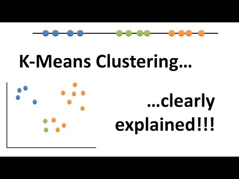](https://www.youtube.com/watch?v=4b5d3muPQmA&ab_channel=StatQuestwithJoshStarmer)\n\n**ISL**\n\n\n[Link to amazon](https://www.amazon.com/Introduction-Statistical-Learning-Applications-Statistics/dp/1071614177/)\n\n**ESL**\n\n\n[Link to amazon](https://www.amazon.com/Elements-Statistical-Learning-Prediction-Statistics/dp/0387848576/)\n\n**Blog**\n\n \n\n[K-Means Clustering From Scratch in Python [Algorithm Explained]](https://www.askpython.com/python/examples/k-means-clustering-from-scratch)\n\n
 \n\n[Elbow Method for optimal value of k in KMeans](https://www.geeksforgeeks.org/elbow-method-for-optimal-value-of-k-in-kmeans/)\n\n
 \n\n[How to Determine the Optimal K for K-Means?](https://medium.com/analytics-vidhya/how-to-determine-the-optimal-k-for-k-means-708505d204eb)\n\n\n\n\n","metadata":{}},{"cell_type":"markdown","source":"# 1. What is KMeans Algorithm\n\nAccording to the ISL book: \"*K-means is a **simple** and **elegant** approach for partioning a data set into **K** **distinct, non-overlapping** clusters*\"\n\nBut what does \"**distinct, non-overlapping clusters**\" mean? \n\nIt means that: \n- \"*each observation belongs to, at least, one of the K clusters*\" and;\n- \"*no observation belongs to more than one cluster*\".\n\nIn other words: each observation must belong to only 1 cluster. It is important to know that the distribution of observations in relation to the clusters **is not random**. For the K-Means algorithm a cluster must be **cohesive**. Such cohesion is related to the **distance** of the points that belong to the cluster in relation to the **center** of this cluster. To simplify the explanation we are going to use the Euclidean distance (although other ways of measuring distance are feasible to be used). \n\nMore formally, this **intra-cluster cohesion** can be measured using the *within-cluster variation* defined by:\n\n
\n\n[How to Determine the Optimal K for K-Means?](https://medium.com/analytics-vidhya/how-to-determine-the-optimal-k-for-k-means-708505d204eb)\n\n\n\n\n","metadata":{}},{"cell_type":"markdown","source":"# 1. What is KMeans Algorithm\n\nAccording to the ISL book: \"*K-means is a **simple** and **elegant** approach for partioning a data set into **K** **distinct, non-overlapping** clusters*\"\n\nBut what does \"**distinct, non-overlapping clusters**\" mean? \n\nIt means that: \n- \"*each observation belongs to, at least, one of the K clusters*\" and;\n- \"*no observation belongs to more than one cluster*\".\n\nIn other words: each observation must belong to only 1 cluster. It is important to know that the distribution of observations in relation to the clusters **is not random**. For the K-Means algorithm a cluster must be **cohesive**. Such cohesion is related to the **distance** of the points that belong to the cluster in relation to the **center** of this cluster. To simplify the explanation we are going to use the Euclidean distance (although other ways of measuring distance are feasible to be used). \n\nMore formally, this **intra-cluster cohesion** can be measured using the *within-cluster variation* defined by:\n\n&space;=&space;\\frac{1}{|C_k|}&space;\\sum_{i,&space;i'&space;\\in&space;C_k}&space;\\sum_{j=1}^{p}&space;(x_{ij}&space;-&space;x_{i',j})^2\") \n\n[Latex codecogs](https://latex.codecogs.com/)\n\nWhere:\n* $W(C_{k})$ is the within-cluster variation\n* $|C_{k}|$ denotes the number of observations in the $k$th cluster\n\nIn practical terms, the above equation means: \"The within-cluster variation for the $k$th cluster is the sum of all the pairwise squared Euclidean distances between the observations in the $k$th cluster\"\n\nNow we can transform the clustering problem into an optimization problem, given by:\n\n
\n\n[Latex codecogs](https://latex.codecogs.com/)\n\nWhere:\n* $W(C_{k})$ is the within-cluster variation\n* $|C_{k}|$ denotes the number of observations in the $k$th cluster\n\nIn practical terms, the above equation means: \"The within-cluster variation for the $k$th cluster is the sum of all the pairwise squared Euclidean distances between the observations in the $k$th cluster\"\n\nNow we can transform the clustering problem into an optimization problem, given by:\n\n\\right\\}\") \n\nWhere $K$ is the number of clusters. \n\nIn practical terms, the above equation means: \"A method to partition the observations into $K$ clusters such that the objective function is minimized\"\n\nFinally we can create our big algorithm composed, basically, by 4 operations:\n\n### K-Means Algorithm\n\n1. Randomly assign k points as out initial centroids\n1. Iterate until the cluster assignments stop changing:\n 1. Calculate the distance between each observation and the centroid and assign each observation to the cluster whose centroid is closest\n 1. Update centroid location by taking the average of the points in each cluster.\n\n**That is all! But first... some considerations**\n\n1. The algorithm, despite having good convergence, **is very sensitive to the starting point**, that is, to the initial points selected as centroids\n1. The algorithm guarantees a **local optimal solution**, so it is important to run the algorithm several times so that it is possible to **estimate the optimal number of clusters** (which is far from an easy problem to solve)\n\nOkay, now we have everything we need to implement our own k-Means algorithm. **Here we go**?\n","metadata":{}},{"cell_type":"code","source":"# general imports\n\nimport os\nimport numpy as np # linear algebra\nimport matplotlib.animation as animation\nimport pandas as pd # data processing, CSV file I/O (e.g. pd.read_csv)\nimport matplotlib.pyplot as plt\nimport seaborn as sns\nfrom tqdm import tqdm\nfrom scipy.spatial.distance import cdist \nimport IPython\nfrom IPython.display import HTML \n\n# sklearn import\nfrom sklearn.datasets import make_classification\nfrom sklearn.cluster import KMeans\nfrom sklearn.metrics import silhouette_score\n\nfrom yellowbrick.cluster.elbow import kelbow_visualizer\n\n\n#some constants\nSEED = 42\nnp.random.seed = SEED","metadata":{"_uuid":"8f2839f25d086af736a60e9eeb907d3b93b6e0e5","_cell_guid":"b1076dfc-b9ad-4769-8c92-a6c4dae69d19","_kg_hide-input":true,"execution":{"iopub.status.busy":"2022-07-09T16:52:58.530808Z","iopub.execute_input":"2022-07-09T16:52:58.531326Z","iopub.status.idle":"2022-07-09T16:52:59.778044Z","shell.execute_reply.started":"2022-07-09T16:52:58.531216Z","shell.execute_reply":"2022-07-09T16:52:59.777247Z"},"trusted":true},"execution_count":null,"outputs":[]},{"cell_type":"markdown","source":"# 2. Implementing our own K-Means\n\nLet's create a hypothetical database. Originally this base contains 400 point. Even if it is a **2-dimensional** dataset, notice that visually **there is not a very well defined separation between the clusters** (and believe me, this is the funnest part).","metadata":{}},{"cell_type":"code","source":"%matplotlib inline\n# didatical dataset\nx, _ = make_classification(n_samples=200,\n n_features=2, \n n_redundant=0, \n n_informative=2, \n n_clusters_per_class=1, \n n_classes=4,\n random_state=SEED)\n\n# Function graph\nplt.figure(figsize=(8,8))\nplt.scatter(x[:, 0], x[:, 1], marker=\"o\", s=30, edgecolor=\"k\")\nplt.legend(['Train points'])\nplt.show()","metadata":{"_kg_hide-input":true,"execution":{"iopub.status.busy":"2022-07-09T16:52:59.780137Z","iopub.execute_input":"2022-07-09T16:52:59.780716Z","iopub.status.idle":"2022-07-09T16:53:00.04346Z","shell.execute_reply.started":"2022-07-09T16:52:59.780676Z","shell.execute_reply":"2022-07-09T16:53:00.042716Z"},"trusted":true},"execution_count":null,"outputs":[]},{"cell_type":"markdown","source":"1. Let's suppose that we are going to separate this dataset into **3 clusters**. The first step then is to **randomly select 3 points** (to be our initial **centroids**), as shown below:","metadata":{}},{"cell_type":"code","source":"K = 3\nidx = np.random.choice(len(x), K, replace=False)\ncentroids = x[idx, :] #Step 1\ncentroids","metadata":{"_kg_hide-input":true,"execution":{"iopub.status.busy":"2022-07-09T16:53:00.044897Z","iopub.execute_input":"2022-07-09T16:53:00.045466Z","iopub.status.idle":"2022-07-09T16:53:00.05434Z","shell.execute_reply.started":"2022-07-09T16:53:00.045429Z","shell.execute_reply":"2022-07-09T16:53:00.053509Z"},"trusted":true},"execution_count":null,"outputs":[]},{"cell_type":"markdown","source":"Let's see where they are...","metadata":{}},{"cell_type":"code","source":"%matplotlib inline\nplt.figure(figsize=(8,8))\nplt.scatter(x[:, 0], x[:, 1], marker=\"o\", s=30, edgecolor=\"k\")\nplt.scatter(centroids[:, 0], centroids[:, 1], marker=\"o\", s=100, edgecolor=\"k\")\nplt.legend(['Train points', 'Inicial centroids'])\nplt.show()","metadata":{"_kg_hide-input":true,"execution":{"iopub.status.busy":"2022-07-09T16:53:00.058242Z","iopub.execute_input":"2022-07-09T16:53:00.058652Z","iopub.status.idle":"2022-07-09T16:53:00.299516Z","shell.execute_reply.started":"2022-07-09T16:53:00.058625Z","shell.execute_reply":"2022-07-09T16:53:00.298855Z"},"trusted":true},"execution_count":null,"outputs":[]},{"cell_type":"markdown","source":"2. Okay... now that we know where they are, **let's calculate the distance between them and all the other points.** (Just an example with 20 points...)\n\nThe first column is the distance from each point to first centroid (and the second columns is the distance from each point to the second centroid, and so on and so on depending on the parameter K)\n\n","metadata":{}},{"cell_type":"code","source":"distances = cdist(x, centroids ,'euclidean') \ndistances[0:20]","metadata":{"_kg_hide-input":true,"execution":{"iopub.status.busy":"2022-07-09T16:53:00.300536Z","iopub.execute_input":"2022-07-09T16:53:00.301467Z","iopub.status.idle":"2022-07-09T16:53:00.309253Z","shell.execute_reply.started":"2022-07-09T16:53:00.301432Z","shell.execute_reply":"2022-07-09T16:53:00.308515Z"},"trusted":true},"execution_count":null,"outputs":[]},{"cell_type":"markdown","source":"Now let's see which cluster each point belongs to...","metadata":{}},{"cell_type":"code","source":"points = np.array([np.argmin(i) for i in distances]) \npoints","metadata":{"_kg_hide-input":true,"execution":{"iopub.status.busy":"2022-07-09T16:53:00.310586Z","iopub.execute_input":"2022-07-09T16:53:00.310937Z","iopub.status.idle":"2022-07-09T16:53:00.320468Z","shell.execute_reply.started":"2022-07-09T16:53:00.310894Z","shell.execute_reply":"2022-07-09T16:53:00.319059Z"},"trusted":true},"execution_count":null,"outputs":[]},{"cell_type":"markdown","source":"Visually it looks like this...","metadata":{}},{"cell_type":"code","source":"%matplotlib inline\nplt.figure(figsize=(8,8))\nplt.scatter(x[:, 0], x[:, 1], c=points, marker=\"o\", s=30, edgecolor=\"k\")\nplt.show()","metadata":{"_kg_hide-input":true,"execution":{"iopub.status.busy":"2022-07-09T16:53:00.321518Z","iopub.execute_input":"2022-07-09T16:53:00.322356Z","iopub.status.idle":"2022-07-09T16:53:00.493101Z","shell.execute_reply.started":"2022-07-09T16:53:00.322322Z","shell.execute_reply":"2022-07-09T16:53:00.492258Z"},"trusted":true},"execution_count":null,"outputs":[]},{"cell_type":"markdown","source":"How about we calculate the **\"within-cluster variation\"**? (the second equation of the introduction)","metadata":{}},{"cell_type":"code","source":"d = {\n 'x0': x[:, 0],\n 'x1': x[:, 1],\n 'c':points\n}\ndf = pd.DataFrame(d)\n\nglobal_whitin = 0\n\n#for each cluster\nfor c in range(3):\n cluster_whitin = 0\n # get all points belonging to that cluster\n local_points = df[df['c'] == c].drop(columns=['c']).to_numpy()\n # number of points that percentile that cluster\n n = local_points.shape[0]\n \n for i in range(n):\n current_point = local_points[i]\n # sum of all distances from all points that belong to that cluster\n cluster_whitin += np.sum(cdist(x, centroids ,'euclidean'))\n \n #divide by the number of points\n cluster_whitin /= n\n \n #accumulate the within of each cluster\n global_whitin += cluster_whitin\n \n \nprint(np.round(global_whitin, 2))","metadata":{"_kg_hide-input":true,"execution":{"iopub.status.busy":"2022-07-09T16:53:00.494653Z","iopub.execute_input":"2022-07-09T16:53:00.494899Z","iopub.status.idle":"2022-07-09T16:53:00.527712Z","shell.execute_reply.started":"2022-07-09T16:53:00.494877Z","shell.execute_reply":"2022-07-09T16:53:00.526851Z"},"trusted":true},"execution_count":null,"outputs":[]},{"cell_type":"markdown","source":"In this step we are able to visualize the **separation boundary between each cluster**....","metadata":{}},{"cell_type":"code","source":"%matplotlib inline\n\nn_points = 50\ngrid_x0 = np.linspace(np.min(x[:, 0]), np.max(x[:, 0]), n_points)\ngrid_x1 = np.linspace(np.min(x[:, 1]), np.max(x[:, 1]), n_points)\nxv, yv = np.meshgrid(grid_x0, grid_x1)\n\ngrid_points = []\n\nfor i in range(n_points):\n for j in range(n_points):\n grid_points.append([xv[i,j],yv[i,j]])\n \ngrid_points = np.array(grid_points)\ngrid_distances = cdist(grid_points, centroids ,'euclidean') \ngrid_clusters = np.array([np.argmin(i) for i in grid_distances]) \nplt.figure(figsize=(8,8))\nplt.scatter(grid_points[:, 0], grid_points[:, 1], c=grid_clusters)\nplt.show()","metadata":{"_kg_hide-input":true,"execution":{"iopub.status.busy":"2022-07-09T16:53:00.529079Z","iopub.execute_input":"2022-07-09T16:53:00.529577Z","iopub.status.idle":"2022-07-09T16:53:00.778103Z","shell.execute_reply.started":"2022-07-09T16:53:00.529545Z","shell.execute_reply":"2022-07-09T16:53:00.77745Z"},"trusted":true},"execution_count":null,"outputs":[]},{"cell_type":"markdown","source":"3. Now let's reposition the centroids based on the mean of the points that make up each cluster","metadata":{}},{"cell_type":"code","source":"centroids_list = []\nfor idx in range(K):\n temp_cent = x[points==idx].mean(axis=0) \n centroids_list.append(temp_cent)\n\nnew_centroids = np.vstack(centroids_list)\nnew_centroids","metadata":{"_kg_hide-input":true,"execution":{"iopub.status.busy":"2022-07-09T16:53:00.780113Z","iopub.execute_input":"2022-07-09T16:53:00.780359Z","iopub.status.idle":"2022-07-09T16:53:00.787116Z","shell.execute_reply.started":"2022-07-09T16:53:00.780338Z","shell.execute_reply":"2022-07-09T16:53:00.786534Z"},"trusted":true},"execution_count":null,"outputs":[]},{"cell_type":"markdown","source":"Let's see where they are (after the update)...","metadata":{}},{"cell_type":"code","source":"%matplotlib inline\nplt.figure(figsize=(8,8))\nplt.scatter(x[:, 0], x[:, 1], marker=\"o\", s=30, edgecolor=\"k\")\nplt.scatter(centroids[:, 0], centroids[:, 1], marker=\"o\", s=100, edgecolor=\"k\")\nplt.scatter(new_centroids[:, 0], new_centroids[:, 1], marker=\"o\", s=100, edgecolor=\"k\")\nplt.legend(['Train points', 'Inicial centroids', 'Updated centroids'])\nplt.show()","metadata":{"_kg_hide-input":true,"execution":{"iopub.status.busy":"2022-07-09T16:53:00.788169Z","iopub.execute_input":"2022-07-09T16:53:00.788831Z","iopub.status.idle":"2022-07-09T16:53:01.002013Z","shell.execute_reply.started":"2022-07-09T16:53:00.788808Z","shell.execute_reply":"2022-07-09T16:53:01.001034Z"},"trusted":true},"execution_count":null,"outputs":[]},{"cell_type":"markdown","source":"Now let's try to visualize in this new centroid configuration","metadata":{}},{"cell_type":"code","source":"%matplotlib inline\ndistances = cdist(x, new_centroids ,'euclidean') \npoints = np.array([np.argmin(i) for i in distances]) \nplt.figure(figsize=(8,8))\nplt.scatter(x[:, 0], x[:, 1], c=points, marker=\"o\", s=30, edgecolor=\"k\")\nplt.show()","metadata":{"_kg_hide-output":false,"_kg_hide-input":true,"execution":{"iopub.status.busy":"2022-07-09T16:53:01.003367Z","iopub.execute_input":"2022-07-09T16:53:01.003715Z","iopub.status.idle":"2022-07-09T16:53:01.167059Z","shell.execute_reply.started":"2022-07-09T16:53:01.003693Z","shell.execute_reply":"2022-07-09T16:53:01.166342Z"},"trusted":true},"execution_count":null,"outputs":[]},{"cell_type":"markdown","source":"How about we calculate the **\"within-cluster variation\"** AGAIN?","metadata":{}},{"cell_type":"code","source":"d = {\n 'x0': x[:, 0],\n 'x1': x[:, 1],\n 'c':points\n}\ndf = pd.DataFrame(d)\n\nglobal_whitin2 = 0\n\n#for each cluster\nfor c in range(3):\n cluster_whitin = 0\n # get all points belonging to that cluster\n local_points = df[df['c'] == c].drop(columns=['c']).to_numpy()\n # number of points that percentile that cluster\n n = local_points.shape[0]\n \n for i in range(n):\n current_point = local_points[i]\n # sum of all distances from all points that belong to that cluster\n cluster_whitin += np.sum(cdist(x, new_centroids ,'euclidean'))\n \n #divide by the number of points\n cluster_whitin /= n\n \n #accumulate the within of each cluster\n global_whitin2 += cluster_whitin\n \n \nprint(f'The first within was {np.round(global_whitin, 2)} and the current is {np.round(global_whitin2, 2)}')","metadata":{"_kg_hide-input":true,"execution":{"iopub.status.busy":"2022-07-09T16:53:01.167964Z","iopub.execute_input":"2022-07-09T16:53:01.168356Z","iopub.status.idle":"2022-07-09T16:53:01.183513Z","shell.execute_reply.started":"2022-07-09T16:53:01.168332Z","shell.execute_reply":"2022-07-09T16:53:01.182841Z"},"trusted":true},"execution_count":null,"outputs":[]},{"cell_type":"markdown","source":"You can also see the difference between the previous and current frontier","metadata":{}},{"cell_type":"code","source":"%matplotlib inline\ngrid_distances = cdist(grid_points, new_centroids ,'euclidean') \nnew_grid_clusters = np.array([np.argmin(i) for i in grid_distances]) \n\nplt.figure(figsize=(16,8))\nplt.subplot(1,2,1)\nplt.title(\"First clusters frontiers\")\nplt.scatter(grid_points[:, 0], grid_points[:, 1], c=grid_clusters)\n\nplt.subplot(1,2,2)\nplt.title(\"Second clusters frontiers\")\nplt.scatter(grid_points[:, 0], grid_points[:, 1], c=new_grid_clusters)","metadata":{"_kg_hide-input":true,"execution":{"iopub.status.busy":"2022-07-09T16:53:01.184342Z","iopub.execute_input":"2022-07-09T16:53:01.184935Z","iopub.status.idle":"2022-07-09T16:53:01.578874Z","shell.execute_reply.started":"2022-07-09T16:53:01.184911Z","shell.execute_reply":"2022-07-09T16:53:01.57822Z"},"trusted":true},"execution_count":null,"outputs":[]},{"cell_type":"markdown","source":"## 2.1 Refactoring - Transforming the code into a function\n\nNow that we've seen how the algorithm works, let's turn it into a function. What we will see next is the code that can be seen in [K-Means Clustering From Scratch in Python [Algorithm Explained]](https://www.askpython.com/python/examples/k-means-clustering-from-scratch) with adaptations so that it is possible to generate an animation.","metadata":{}},{"cell_type":"code","source":"#Function to implement steps given in previous section\ndef kmeans(x, k=3, no_of_iterations=10):\n \n # centroids story list\n centroids_history = []\n points_history = []\n \n idx = np.random.choice(len(x), k, replace=False)\n #Randomly choosing Centroids \n centroids = x[idx, :] #Step 1\n centroids_history.append(centroids)\n \n #finding the distance between centroids and all the data points\n distances = cdist(x, centroids ,'euclidean') #Step 2\n \n #Centroid with the minimum Distance\n points = np.array([np.argmin(i) for i in distances]) #Step 3\n points_history.append(points)\n \n #Repeating the above steps for a defined number of iterations\n #Step 4\n for _ in range(no_of_iterations): \n centroids = []\n for idx in range(k):\n #Updating Centroids by taking mean of Cluster it belongs to\n temp_cent = x[points==idx].mean(axis=0) \n centroids.append(temp_cent)\n \n centroids = np.vstack(centroids) #Updated Centroids \n centroids_history.append(centroids)\n \n \n distances = cdist(x, centroids ,'euclidean')\n points = np.array([np.argmin(i) for i in distances])\n points_history.append(points)\n\n \n return points, points_history, centroids_history","metadata":{"_kg_hide-input":false,"execution":{"iopub.status.busy":"2022-07-09T16:53:01.580156Z","iopub.execute_input":"2022-07-09T16:53:01.581189Z","iopub.status.idle":"2022-07-09T16:53:01.592653Z","shell.execute_reply.started":"2022-07-09T16:53:01.581158Z","shell.execute_reply":"2022-07-09T16:53:01.591315Z"},"trusted":true},"execution_count":null,"outputs":[]},{"cell_type":"markdown","source":"## 2.2 Testing the function in an animated way!!!\n\nUse the player below to see how the centroids move (in each iteration) and how this affects the distribution between clustersUse the player below to see how the centroids move (in each iteration) and how this affects the distribution between clusters","metadata":{}},{"cell_type":"code","source":"%matplotlib notebook\n\npoints, points_history, centroids_history = kmeans(x, k=3, no_of_iterations=10)\n\nlimits_x = (np.min(x[:, 0]), np.max(x[:, 0]))\nlimits_y = (np.min(x[:, 1]), np.max(x[:, 1]))\n\nsteps = 10\nfig, ax = plt.subplots(figsize=(8,8))\ndef animate(i):\n fig.clear()\n ax = fig.add_subplot(111, aspect='equal', autoscale_on=False, xlim=limits_x, ylim=limits_y)\n ax.set_title(f\"Iteration {i}\")\n ax.set_xlim(np.min(x[:, 0]), np.max(x[:, 0]))\n ax.set_ylim(np.min(x[:, 1]), np.max(x[:, 1]))\n s = ax.scatter(x[:, 0], x[:, 1], c=points_history[i], marker=\"o\", s=30, edgecolor=\"k\")\n ax.scatter(centroids_history[i][:, 0], centroids_history[i][:, 1], marker=\"o\", s=100, edgecolor=\"k\")\n ax.legend(['Train points', 'Centroids'])\n\n \nani = animation.FuncAnimation(fig, animate, interval=250, frames=range(steps)) \nHTML(ani.to_jshtml())","metadata":{"_kg_hide-input":true,"execution":{"iopub.status.busy":"2022-07-09T16:53:01.595626Z","iopub.execute_input":"2022-07-09T16:53:01.595911Z","iopub.status.idle":"2022-07-09T16:53:03.258507Z","shell.execute_reply.started":"2022-07-09T16:53:01.595879Z","shell.execute_reply":"2022-07-09T16:53:03.257635Z"},"trusted":true},"execution_count":null,"outputs":[]},{"cell_type":"markdown","source":"# 3. Using sklearn\n\n**Disclaimer**\n\nNow let's use a professional package to find the clusters. As stated earlier, the algorithm **is very sensitive to the starting point**. Also, the function we created has a didactic purpose and not a professional one, so the results will vary a lot, ok?\n\n\nRunning K-Means using sklearn **is simpler than you might think**... follow the code below with a configuration similar to what we did in the previous experiment...","metadata":{}},{"cell_type":"code","source":"# Instantiating the KMeans class object\nkmeans = KMeans(n_clusters=3, \n init='random',\n random_state=SEED)\n# Fitting the points\nkmeans.fit(x)\npoints = kmeans.labels_\ncentroids = kmeans.cluster_centers_","metadata":{"execution":{"iopub.status.busy":"2022-07-09T16:53:03.260027Z","iopub.execute_input":"2022-07-09T16:53:03.260296Z","iopub.status.idle":"2022-07-09T16:53:03.296486Z","shell.execute_reply.started":"2022-07-09T16:53:03.26027Z","shell.execute_reply":"2022-07-09T16:53:03.295809Z"},"trusted":true},"execution_count":null,"outputs":[]},{"cell_type":"markdown","source":"Let's now see the results, first how the clusters turned out...","metadata":{}},{"cell_type":"code","source":"%matplotlib inline\nplt.figure(figsize=(8,8))\nplt.scatter(x[:, 0], x[:, 1], c=points, marker=\"o\", s=30, edgecolor=\"k\")\nplt.scatter(centroids[:, 0], centroids[:, 1], marker=\"o\", s=100, edgecolor=\"k\")\nplt.legend(['Train points', 'Centroids'])\nplt.show()","metadata":{"execution":{"iopub.status.busy":"2022-07-09T16:53:03.297734Z","iopub.execute_input":"2022-07-09T16:53:03.298175Z","iopub.status.idle":"2022-07-09T16:53:03.493203Z","shell.execute_reply.started":"2022-07-09T16:53:03.298148Z","shell.execute_reply":"2022-07-09T16:53:03.49178Z"},"trusted":true},"execution_count":null,"outputs":[]},{"cell_type":"markdown","source":"Now how is the separation boundary between the clusters","metadata":{}},{"cell_type":"code","source":"grid_points = np.array(grid_points)\ngrid_distances = cdist(grid_points, centroids ,'euclidean') \ngrid_clusters = np.array([np.argmin(i) for i in grid_distances]) \nplt.figure(figsize=(8,8))\nplt.scatter(grid_points[:, 0], grid_points[:, 1], c=grid_clusters)\nplt.show()","metadata":{"execution":{"iopub.status.busy":"2022-07-09T16:53:03.4947Z","iopub.execute_input":"2022-07-09T16:53:03.494931Z","iopub.status.idle":"2022-07-09T16:53:03.715164Z","shell.execute_reply.started":"2022-07-09T16:53:03.49491Z","shell.execute_reply":"2022-07-09T16:53:03.714041Z"},"trusted":true},"execution_count":null,"outputs":[]},{"cell_type":"markdown","source":"## 3.1 Choosing the K parameter\n\nSo far using k=3 (only to visualize the behavior of the algorithm). But is this the best parameter? Maybe so, maybe not, but the most likely answer is \"I don't know\"... So let's try some different ways to choose this important parameter!\n\n### 3.1.1 Elbow Method using intertia and distortion\n\nAccording to [wikipedia](https://en.wikipedia.org/wiki/Elbow_method_(clustering)):\n\n> Using the \"elbow\" or \"knee of a curve\" as a cutoff point **is a common heuristic** in mathematical optimization to choose a point where diminishing **returns are no longer worth the additional cost**. In clustering, this means one should choose a number of clusters so that **adding another cluster doesn't give much better modeling of the data**.\n\nHere we will use 2 methods to calculate the cost: the intertia and the distortion\n\nAccording to [geeksforgeeks.org](https://www.geeksforgeeks.org/elbow-method-for-optimal-value-of-k-in-kmeans/):\n\n> 1. **Distortion:** It is calculated as the average of the squared distances from the cluster centers of the respective clusters. Typically, the Euclidean distance metric is used.\n> 2. **Inertia:** It is the sum of squared distances of samples to their closest cluster center.\n\n\nHere we will use the code based on [geeksforgeeks.org](https://www.geeksforgeeks.org/elbow-method-for-optimal-value-of-k-in-kmeans/)","metadata":{}},{"cell_type":"code","source":"distortions = []\ninertias = []\n\nK = range(1, 15)\nfor k in tqdm(K):\n # Building and fitting the model\n kmeans = KMeans(n_clusters=k, \n init='random',\n random_state=SEED)\n kmeans.fit(x)\n \n dist = sum(np.min(cdist(x, kmeans.cluster_centers_,'euclidean'), axis=1)) / x.shape[0]\n inertia = kmeans.inertia_\n \n distortions.append(dist)\n inertias.append(inertia)","metadata":{"execution":{"iopub.status.busy":"2022-07-09T16:53:03.717552Z","iopub.execute_input":"2022-07-09T16:53:03.717808Z","iopub.status.idle":"2022-07-09T16:53:04.163494Z","shell.execute_reply.started":"2022-07-09T16:53:03.717786Z","shell.execute_reply":"2022-07-09T16:53:04.162749Z"},"trusted":true},"execution_count":null,"outputs":[]},{"cell_type":"markdown","source":"First, let's use the **distortion measure**\n\nThe graph below shows that from **5 clusters onwards**, the distortion value does not vary much... (which helps us to understand that **there may be 5 distinct clusters** in this dataset)","metadata":{}},{"cell_type":"code","source":"plt.figure(figsize=(8,8))\nplt.plot(K, distortions, 'x-')\nplt.plot(range(2, 15), np.diff(distortions), 'x-')\nplt.xlabel('Values of K')\nplt.ylabel('Distortion')\nplt.title('The Elbow Method using Distortion')\nplt.legend(['Distortion', 'Diff between current and previous distortion'])\nplt.show()","metadata":{"_kg_hide-input":true,"execution":{"iopub.status.busy":"2022-07-09T16:53:04.166804Z","iopub.execute_input":"2022-07-09T16:53:04.168522Z","iopub.status.idle":"2022-07-09T16:53:04.370452Z","shell.execute_reply.started":"2022-07-09T16:53:04.168491Z","shell.execute_reply":"2022-07-09T16:53:04.369499Z"},"trusted":true},"execution_count":null,"outputs":[]},{"cell_type":"markdown","source":"See how interesting... for the inertia measure the **result is similar**... above 5 clusters the inertia measure is almost constant","metadata":{}},{"cell_type":"code","source":"plt.figure(figsize=(8,8))\nplt.plot(K, inertias, 'x-')\nplt.plot(range(2, 15), np.diff(inertias), 'x-')\nplt.xlabel('Values of K')\nplt.ylabel('Inertia')\nplt.title('The Elbow Method using Inertia')\nplt.legend(['Inertia', 'Diff between current and previous inertia'])\nplt.show()","metadata":{"_kg_hide-input":true,"execution":{"iopub.status.busy":"2022-07-09T16:53:04.371626Z","iopub.execute_input":"2022-07-09T16:53:04.371888Z","iopub.status.idle":"2022-07-09T16:53:04.582755Z","shell.execute_reply.started":"2022-07-09T16:53:04.371862Z","shell.execute_reply":"2022-07-09T16:53:04.581707Z"},"trusted":true},"execution_count":null,"outputs":[]},{"cell_type":"markdown","source":"### 3.1.2 The Silhouette Method\n\nNow let's try the silhouette method. According to [Silhouette (clustering)](https://en.wikipedia.org/wiki/Silhouette_(clustering)):\n\n> The silhouette ranges from −1 to +1, where a high value indicates that the object is well matched to its own cluster and poorly matched to neighboring clusters. \n\nHere we will use the code based on [How to Determine the Optimal K for K-Means?](https://medium.com/analytics-vidhya/how-to-determine-the-optimal-k-for-k-means-708505d204eb)","metadata":{}},{"cell_type":"markdown","source":"According to the graph below, the silhouette score reaches its **maximum point** with **k=3** (which helps us to understand that there may be 3 distinct clusters in this dataset)","metadata":{}},{"cell_type":"code","source":"sil = []\nkmax = 15\n\nfor k in range(2, kmax+1):\n kmeans = KMeans(n_clusters=k, \n init='random',\n random_state=SEED)\n kmeans.fit(x)\n labels = kmeans.labels_\n sil.append(silhouette_score(x, labels, metric = 'euclidean', random_state=SEED))","metadata":{"execution":{"iopub.status.busy":"2022-07-09T16:53:04.583826Z","iopub.execute_input":"2022-07-09T16:53:04.584145Z","iopub.status.idle":"2022-07-09T16:53:06.322678Z","shell.execute_reply.started":"2022-07-09T16:53:04.584115Z","shell.execute_reply":"2022-07-09T16:53:06.321913Z"},"trusted":true},"execution_count":null,"outputs":[]},{"cell_type":"code","source":"plt.figure(figsize=(8,8))\nplt.plot(range(2, kmax+1), sil, 'x-')\nplt.xlabel('Values of K')\nplt.ylabel('Silhouette score')\nplt.title('The Silhouette Method')\nplt.show()","metadata":{"_kg_hide-input":true,"execution":{"iopub.status.busy":"2022-07-09T16:53:06.323976Z","iopub.execute_input":"2022-07-09T16:53:06.325623Z","iopub.status.idle":"2022-07-09T16:53:06.485711Z","shell.execute_reply.started":"2022-07-09T16:53:06.325588Z","shell.execute_reply":"2022-07-09T16:53:06.484877Z"},"trusted":true},"execution_count":null,"outputs":[]},{"cell_type":"markdown","source":"# 4 Tabular Playground Series - Jul 2022\n\nNow it's time to apply all the knowledge seen so far in our TPS :-)","metadata":{}},{"cell_type":"code","source":"df = pd.read_csv('/kaggle/input/tabular-playground-series-jul-2022/data.csv')\nprint(df.shape)\ndf.head()","metadata":{"execution":{"iopub.status.busy":"2022-07-09T16:53:06.487075Z","iopub.execute_input":"2022-07-09T16:53:06.487641Z","iopub.status.idle":"2022-07-09T16:53:07.437153Z","shell.execute_reply.started":"2022-07-09T16:53:06.487608Z","shell.execute_reply":"2022-07-09T16:53:07.436166Z"},"trusted":true},"execution_count":null,"outputs":[]},{"cell_type":"markdown","source":"Let's make a little exploratory data analysis + data engineering","metadata":{}},{"cell_type":"code","source":"count = 1\nfor c in df.columns:\n print(f'{count} - {c}')\n print(f'- # of unique elements: {df[c].nunique()}')\n print(f'- Sample: {df[c].unique()[0:20]}')\n print(f'- Dtype: {df[c].dtype}')\n print(f'- # of missing values: {df[c].isnull().sum()} of {df.shape[0]}')\n print(f'- % of missing values: {np.round(df[c].isnull().sum() / df.shape[0], 3)}')\n \n \n if df[c].dtype == int or df[c].dtype == float:\n s = \"- Statistics:\\n\"\n\n me = np.round(df[c].mean(), 2)\n st = np.round(df[c].std(), 2)\n s += f\"-- Mean (std): {me} ({st})\\n\"\n\n q1 = np.round(df[c].quantile(0.25), 2)\n q2 = np.round(df[c].quantile(0.5), 2)\n q3 = np.round(df[c].quantile(0.75), 2)\n s += f\"-- Quantiles: q1={q1}, q2={q2}, q3={q3}\\n\"\n s += f\"-- Min {df[c].min()}\\n\"\n s += f\"-- Max {df[c].max()}\" \n print(s)\n \n print('='*30)\n count += 1","metadata":{"_kg_hide-input":true,"execution":{"iopub.status.busy":"2022-07-09T16:53:07.438293Z","iopub.execute_input":"2022-07-09T16:53:07.438571Z","iopub.status.idle":"2022-07-09T16:53:07.891266Z","shell.execute_reply.started":"2022-07-09T16:53:07.438543Z","shell.execute_reply":"2022-07-09T16:53:07.890307Z"},"trusted":true},"execution_count":null,"outputs":[]},{"cell_type":"markdown","source":"**Some conclusions:**\n* There are no missing values\n* Most of the variables seem to have a normal distribution with mean 0 and standard deviation 1\n* Very few variables have discrepant mean and median (what can lead to a skewed distribution)","metadata":{}},{"cell_type":"markdown","source":"## 4.1 Applying K-Means\n\nTo make the job a little easier, I'm going to use the [Yellowbrick](https://www.scikit-yb.org/en/latest/index.html) package which has great ways of visualizing data and models","metadata":{}},{"cell_type":"code","source":"df_model = df.drop(columns=['id'])","metadata":{"_kg_hide-input":true,"execution":{"iopub.status.busy":"2022-07-09T16:53:07.892625Z","iopub.execute_input":"2022-07-09T16:53:07.892855Z","iopub.status.idle":"2022-07-09T16:53:07.901861Z","shell.execute_reply.started":"2022-07-09T16:53:07.892833Z","shell.execute_reply":"2022-07-09T16:53:07.900503Z"},"trusted":true},"execution_count":null,"outputs":[]},{"cell_type":"markdown","source":"### 4.1.1 Elbow Method (distortion)","metadata":{}},{"cell_type":"code","source":"# Use the quick method and immediately show the figure\nkmeans = KMeans(init='random',random_state=SEED)\nelbow = kelbow_visualizer(kmeans, df_model, k=(2,10), timings=False, metric='distortion')","metadata":{"execution":{"iopub.status.busy":"2022-07-09T16:53:07.903591Z","iopub.execute_input":"2022-07-09T16:53:07.903979Z","iopub.status.idle":"2022-07-09T16:53:29.188263Z","shell.execute_reply.started":"2022-07-09T16:53:07.903951Z","shell.execute_reply":"2022-07-09T16:53:29.187524Z"},"trusted":true},"execution_count":null,"outputs":[]},{"cell_type":"markdown","source":"### 4.1.2 Silhouette","metadata":{}},{"cell_type":"code","source":"sil = []\nkmax = 10\n\nfor k in tqdm(range(2, kmax+1)):\n kmeans = KMeans(n_clusters=k, \n init='random',\n random_state=SEED)\n kmeans.fit(df_model)\n labels = kmeans.labels_\n sil.append(silhouette_score(df_model, labels, metric = 'euclidean', random_state=SEED))","metadata":{"execution":{"iopub.status.busy":"2022-07-09T17:00:32.04361Z","iopub.execute_input":"2022-07-09T17:00:32.043906Z","iopub.status.idle":"2022-07-09T17:14:37.15191Z","shell.execute_reply.started":"2022-07-09T17:00:32.043879Z","shell.execute_reply":"2022-07-09T17:14:37.150847Z"},"trusted":true},"execution_count":null,"outputs":[]},{"cell_type":"code","source":"plt.figure(figsize=(8,8))\nplt.plot(range(2, kmax+1), sil, 'x-')\nplt.xlabel('Values of K')\nplt.ylabel('Silhouette score')\nplt.title('The Silhouette Method')\nplt.show()","metadata":{"_kg_hide-input":true,"execution":{"iopub.status.busy":"2022-07-09T17:14:37.333932Z","iopub.execute_input":"2022-07-09T17:14:37.334264Z","iopub.status.idle":"2022-07-09T17:14:37.491116Z","shell.execute_reply.started":"2022-07-09T17:14:37.334233Z","shell.execute_reply":"2022-07-09T17:14:37.49013Z"},"trusted":true},"execution_count":null,"outputs":[]},{"cell_type":"markdown","source":"### 4.1.3 Elbow Method (calinski_harabasz)","metadata":{}},{"cell_type":"code","source":"# Use the quick method and immediately show the figure\nkmeans = KMeans(init='random',random_state=SEED)\nelbow = kelbow_visualizer(kmeans, df_model, k=(2,10), timings=False, metric='calinski_harabasz')","metadata":{"execution":{"iopub.status.busy":"2022-07-09T16:54:50.979918Z","iopub.execute_input":"2022-07-09T16:54:50.98026Z","iopub.status.idle":"2022-07-09T16:55:11.455349Z","shell.execute_reply.started":"2022-07-09T16:54:50.980235Z","shell.execute_reply":"2022-07-09T16:55:11.454423Z"},"trusted":true},"execution_count":null,"outputs":[]},{"cell_type":"markdown","source":"Based on the graphs above it **is likely that there are only 2 groups in the dataset** (we will unfortunately never know how many groups there actually are, but no problem, the important thing is to learn, right?).","metadata":{}},{"cell_type":"markdown","source":"## 4.2 Generating the final solution","metadata":{}},{"cell_type":"code","source":"kmeans = KMeans(n_clusters=2, \n init='random',\n random_state=SEED)\nkmeans.fit(df_model)\nlabels = kmeans.labels_\n\ndf['Predicted'] = labels\ndf[['id', 'Predicted']].head(10)","metadata":{"execution":{"iopub.status.busy":"2022-07-09T17:19:33.318841Z","iopub.execute_input":"2022-07-09T17:19:33.31922Z","iopub.status.idle":"2022-07-09T17:19:34.195524Z","shell.execute_reply.started":"2022-07-09T17:19:33.319191Z","shell.execute_reply":"2022-07-09T17:19:34.194422Z"},"trusted":true},"execution_count":null,"outputs":[]},{"cell_type":"code","source":"# Save submission\ndf = df[['id', 'Predicted']]\ndf.to_csv('submission.csv', index=False, header=True)","metadata":{"execution":{"iopub.status.busy":"2022-07-09T17:20:35.004622Z","iopub.execute_input":"2022-07-09T17:20:35.004922Z","iopub.status.idle":"2022-07-09T17:20:35.105652Z","shell.execute_reply.started":"2022-07-09T17:20:35.004897Z","shell.execute_reply":"2022-07-09T17:20:35.104295Z"},"trusted":true},"execution_count":null,"outputs":[]},{"cell_type":"markdown","source":"# 5. (Some) Conclusions:\n\n1. I tried to show here the main concepts related to the K-Means algorithm\n1. If you have any suggestions (or criticisms), leave them in the comments...\n1. We can see that the algorithm is very simple and, at the same time, very competitive!","metadata":{}}]}
\n\nWhere $K$ is the number of clusters. \n\nIn practical terms, the above equation means: \"A method to partition the observations into $K$ clusters such that the objective function is minimized\"\n\nFinally we can create our big algorithm composed, basically, by 4 operations:\n\n### K-Means Algorithm\n\n1. Randomly assign k points as out initial centroids\n1. Iterate until the cluster assignments stop changing:\n 1. Calculate the distance between each observation and the centroid and assign each observation to the cluster whose centroid is closest\n 1. Update centroid location by taking the average of the points in each cluster.\n\n**That is all! But first... some considerations**\n\n1. The algorithm, despite having good convergence, **is very sensitive to the starting point**, that is, to the initial points selected as centroids\n1. The algorithm guarantees a **local optimal solution**, so it is important to run the algorithm several times so that it is possible to **estimate the optimal number of clusters** (which is far from an easy problem to solve)\n\nOkay, now we have everything we need to implement our own k-Means algorithm. **Here we go**?\n","metadata":{}},{"cell_type":"code","source":"# general imports\n\nimport os\nimport numpy as np # linear algebra\nimport matplotlib.animation as animation\nimport pandas as pd # data processing, CSV file I/O (e.g. pd.read_csv)\nimport matplotlib.pyplot as plt\nimport seaborn as sns\nfrom tqdm import tqdm\nfrom scipy.spatial.distance import cdist \nimport IPython\nfrom IPython.display import HTML \n\n# sklearn import\nfrom sklearn.datasets import make_classification\nfrom sklearn.cluster import KMeans\nfrom sklearn.metrics import silhouette_score\n\nfrom yellowbrick.cluster.elbow import kelbow_visualizer\n\n\n#some constants\nSEED = 42\nnp.random.seed = SEED","metadata":{"_uuid":"8f2839f25d086af736a60e9eeb907d3b93b6e0e5","_cell_guid":"b1076dfc-b9ad-4769-8c92-a6c4dae69d19","_kg_hide-input":true,"execution":{"iopub.status.busy":"2022-07-09T16:52:58.530808Z","iopub.execute_input":"2022-07-09T16:52:58.531326Z","iopub.status.idle":"2022-07-09T16:52:59.778044Z","shell.execute_reply.started":"2022-07-09T16:52:58.531216Z","shell.execute_reply":"2022-07-09T16:52:59.777247Z"},"trusted":true},"execution_count":null,"outputs":[]},{"cell_type":"markdown","source":"# 2. Implementing our own K-Means\n\nLet's create a hypothetical database. Originally this base contains 400 point. Even if it is a **2-dimensional** dataset, notice that visually **there is not a very well defined separation between the clusters** (and believe me, this is the funnest part).","metadata":{}},{"cell_type":"code","source":"%matplotlib inline\n# didatical dataset\nx, _ = make_classification(n_samples=200,\n n_features=2, \n n_redundant=0, \n n_informative=2, \n n_clusters_per_class=1, \n n_classes=4,\n random_state=SEED)\n\n# Function graph\nplt.figure(figsize=(8,8))\nplt.scatter(x[:, 0], x[:, 1], marker=\"o\", s=30, edgecolor=\"k\")\nplt.legend(['Train points'])\nplt.show()","metadata":{"_kg_hide-input":true,"execution":{"iopub.status.busy":"2022-07-09T16:52:59.780137Z","iopub.execute_input":"2022-07-09T16:52:59.780716Z","iopub.status.idle":"2022-07-09T16:53:00.04346Z","shell.execute_reply.started":"2022-07-09T16:52:59.780676Z","shell.execute_reply":"2022-07-09T16:53:00.042716Z"},"trusted":true},"execution_count":null,"outputs":[]},{"cell_type":"markdown","source":"1. Let's suppose that we are going to separate this dataset into **3 clusters**. The first step then is to **randomly select 3 points** (to be our initial **centroids**), as shown below:","metadata":{}},{"cell_type":"code","source":"K = 3\nidx = np.random.choice(len(x), K, replace=False)\ncentroids = x[idx, :] #Step 1\ncentroids","metadata":{"_kg_hide-input":true,"execution":{"iopub.status.busy":"2022-07-09T16:53:00.044897Z","iopub.execute_input":"2022-07-09T16:53:00.045466Z","iopub.status.idle":"2022-07-09T16:53:00.05434Z","shell.execute_reply.started":"2022-07-09T16:53:00.045429Z","shell.execute_reply":"2022-07-09T16:53:00.053509Z"},"trusted":true},"execution_count":null,"outputs":[]},{"cell_type":"markdown","source":"Let's see where they are...","metadata":{}},{"cell_type":"code","source":"%matplotlib inline\nplt.figure(figsize=(8,8))\nplt.scatter(x[:, 0], x[:, 1], marker=\"o\", s=30, edgecolor=\"k\")\nplt.scatter(centroids[:, 0], centroids[:, 1], marker=\"o\", s=100, edgecolor=\"k\")\nplt.legend(['Train points', 'Inicial centroids'])\nplt.show()","metadata":{"_kg_hide-input":true,"execution":{"iopub.status.busy":"2022-07-09T16:53:00.058242Z","iopub.execute_input":"2022-07-09T16:53:00.058652Z","iopub.status.idle":"2022-07-09T16:53:00.299516Z","shell.execute_reply.started":"2022-07-09T16:53:00.058625Z","shell.execute_reply":"2022-07-09T16:53:00.298855Z"},"trusted":true},"execution_count":null,"outputs":[]},{"cell_type":"markdown","source":"2. Okay... now that we know where they are, **let's calculate the distance between them and all the other points.** (Just an example with 20 points...)\n\nThe first column is the distance from each point to first centroid (and the second columns is the distance from each point to the second centroid, and so on and so on depending on the parameter K)\n\n","metadata":{}},{"cell_type":"code","source":"distances = cdist(x, centroids ,'euclidean') \ndistances[0:20]","metadata":{"_kg_hide-input":true,"execution":{"iopub.status.busy":"2022-07-09T16:53:00.300536Z","iopub.execute_input":"2022-07-09T16:53:00.301467Z","iopub.status.idle":"2022-07-09T16:53:00.309253Z","shell.execute_reply.started":"2022-07-09T16:53:00.301432Z","shell.execute_reply":"2022-07-09T16:53:00.308515Z"},"trusted":true},"execution_count":null,"outputs":[]},{"cell_type":"markdown","source":"Now let's see which cluster each point belongs to...","metadata":{}},{"cell_type":"code","source":"points = np.array([np.argmin(i) for i in distances]) \npoints","metadata":{"_kg_hide-input":true,"execution":{"iopub.status.busy":"2022-07-09T16:53:00.310586Z","iopub.execute_input":"2022-07-09T16:53:00.310937Z","iopub.status.idle":"2022-07-09T16:53:00.320468Z","shell.execute_reply.started":"2022-07-09T16:53:00.310894Z","shell.execute_reply":"2022-07-09T16:53:00.319059Z"},"trusted":true},"execution_count":null,"outputs":[]},{"cell_type":"markdown","source":"Visually it looks like this...","metadata":{}},{"cell_type":"code","source":"%matplotlib inline\nplt.figure(figsize=(8,8))\nplt.scatter(x[:, 0], x[:, 1], c=points, marker=\"o\", s=30, edgecolor=\"k\")\nplt.show()","metadata":{"_kg_hide-input":true,"execution":{"iopub.status.busy":"2022-07-09T16:53:00.321518Z","iopub.execute_input":"2022-07-09T16:53:00.322356Z","iopub.status.idle":"2022-07-09T16:53:00.493101Z","shell.execute_reply.started":"2022-07-09T16:53:00.322322Z","shell.execute_reply":"2022-07-09T16:53:00.492258Z"},"trusted":true},"execution_count":null,"outputs":[]},{"cell_type":"markdown","source":"How about we calculate the **\"within-cluster variation\"**? (the second equation of the introduction)","metadata":{}},{"cell_type":"code","source":"d = {\n 'x0': x[:, 0],\n 'x1': x[:, 1],\n 'c':points\n}\ndf = pd.DataFrame(d)\n\nglobal_whitin = 0\n\n#for each cluster\nfor c in range(3):\n cluster_whitin = 0\n # get all points belonging to that cluster\n local_points = df[df['c'] == c].drop(columns=['c']).to_numpy()\n # number of points that percentile that cluster\n n = local_points.shape[0]\n \n for i in range(n):\n current_point = local_points[i]\n # sum of all distances from all points that belong to that cluster\n cluster_whitin += np.sum(cdist(x, centroids ,'euclidean'))\n \n #divide by the number of points\n cluster_whitin /= n\n \n #accumulate the within of each cluster\n global_whitin += cluster_whitin\n \n \nprint(np.round(global_whitin, 2))","metadata":{"_kg_hide-input":true,"execution":{"iopub.status.busy":"2022-07-09T16:53:00.494653Z","iopub.execute_input":"2022-07-09T16:53:00.494899Z","iopub.status.idle":"2022-07-09T16:53:00.527712Z","shell.execute_reply.started":"2022-07-09T16:53:00.494877Z","shell.execute_reply":"2022-07-09T16:53:00.526851Z"},"trusted":true},"execution_count":null,"outputs":[]},{"cell_type":"markdown","source":"In this step we are able to visualize the **separation boundary between each cluster**....","metadata":{}},{"cell_type":"code","source":"%matplotlib inline\n\nn_points = 50\ngrid_x0 = np.linspace(np.min(x[:, 0]), np.max(x[:, 0]), n_points)\ngrid_x1 = np.linspace(np.min(x[:, 1]), np.max(x[:, 1]), n_points)\nxv, yv = np.meshgrid(grid_x0, grid_x1)\n\ngrid_points = []\n\nfor i in range(n_points):\n for j in range(n_points):\n grid_points.append([xv[i,j],yv[i,j]])\n \ngrid_points = np.array(grid_points)\ngrid_distances = cdist(grid_points, centroids ,'euclidean') \ngrid_clusters = np.array([np.argmin(i) for i in grid_distances]) \nplt.figure(figsize=(8,8))\nplt.scatter(grid_points[:, 0], grid_points[:, 1], c=grid_clusters)\nplt.show()","metadata":{"_kg_hide-input":true,"execution":{"iopub.status.busy":"2022-07-09T16:53:00.529079Z","iopub.execute_input":"2022-07-09T16:53:00.529577Z","iopub.status.idle":"2022-07-09T16:53:00.778103Z","shell.execute_reply.started":"2022-07-09T16:53:00.529545Z","shell.execute_reply":"2022-07-09T16:53:00.77745Z"},"trusted":true},"execution_count":null,"outputs":[]},{"cell_type":"markdown","source":"3. Now let's reposition the centroids based on the mean of the points that make up each cluster","metadata":{}},{"cell_type":"code","source":"centroids_list = []\nfor idx in range(K):\n temp_cent = x[points==idx].mean(axis=0) \n centroids_list.append(temp_cent)\n\nnew_centroids = np.vstack(centroids_list)\nnew_centroids","metadata":{"_kg_hide-input":true,"execution":{"iopub.status.busy":"2022-07-09T16:53:00.780113Z","iopub.execute_input":"2022-07-09T16:53:00.780359Z","iopub.status.idle":"2022-07-09T16:53:00.787116Z","shell.execute_reply.started":"2022-07-09T16:53:00.780338Z","shell.execute_reply":"2022-07-09T16:53:00.786534Z"},"trusted":true},"execution_count":null,"outputs":[]},{"cell_type":"markdown","source":"Let's see where they are (after the update)...","metadata":{}},{"cell_type":"code","source":"%matplotlib inline\nplt.figure(figsize=(8,8))\nplt.scatter(x[:, 0], x[:, 1], marker=\"o\", s=30, edgecolor=\"k\")\nplt.scatter(centroids[:, 0], centroids[:, 1], marker=\"o\", s=100, edgecolor=\"k\")\nplt.scatter(new_centroids[:, 0], new_centroids[:, 1], marker=\"o\", s=100, edgecolor=\"k\")\nplt.legend(['Train points', 'Inicial centroids', 'Updated centroids'])\nplt.show()","metadata":{"_kg_hide-input":true,"execution":{"iopub.status.busy":"2022-07-09T16:53:00.788169Z","iopub.execute_input":"2022-07-09T16:53:00.788831Z","iopub.status.idle":"2022-07-09T16:53:01.002013Z","shell.execute_reply.started":"2022-07-09T16:53:00.788808Z","shell.execute_reply":"2022-07-09T16:53:01.001034Z"},"trusted":true},"execution_count":null,"outputs":[]},{"cell_type":"markdown","source":"Now let's try to visualize in this new centroid configuration","metadata":{}},{"cell_type":"code","source":"%matplotlib inline\ndistances = cdist(x, new_centroids ,'euclidean') \npoints = np.array([np.argmin(i) for i in distances]) \nplt.figure(figsize=(8,8))\nplt.scatter(x[:, 0], x[:, 1], c=points, marker=\"o\", s=30, edgecolor=\"k\")\nplt.show()","metadata":{"_kg_hide-output":false,"_kg_hide-input":true,"execution":{"iopub.status.busy":"2022-07-09T16:53:01.003367Z","iopub.execute_input":"2022-07-09T16:53:01.003715Z","iopub.status.idle":"2022-07-09T16:53:01.167059Z","shell.execute_reply.started":"2022-07-09T16:53:01.003693Z","shell.execute_reply":"2022-07-09T16:53:01.166342Z"},"trusted":true},"execution_count":null,"outputs":[]},{"cell_type":"markdown","source":"How about we calculate the **\"within-cluster variation\"** AGAIN?","metadata":{}},{"cell_type":"code","source":"d = {\n 'x0': x[:, 0],\n 'x1': x[:, 1],\n 'c':points\n}\ndf = pd.DataFrame(d)\n\nglobal_whitin2 = 0\n\n#for each cluster\nfor c in range(3):\n cluster_whitin = 0\n # get all points belonging to that cluster\n local_points = df[df['c'] == c].drop(columns=['c']).to_numpy()\n # number of points that percentile that cluster\n n = local_points.shape[0]\n \n for i in range(n):\n current_point = local_points[i]\n # sum of all distances from all points that belong to that cluster\n cluster_whitin += np.sum(cdist(x, new_centroids ,'euclidean'))\n \n #divide by the number of points\n cluster_whitin /= n\n \n #accumulate the within of each cluster\n global_whitin2 += cluster_whitin\n \n \nprint(f'The first within was {np.round(global_whitin, 2)} and the current is {np.round(global_whitin2, 2)}')","metadata":{"_kg_hide-input":true,"execution":{"iopub.status.busy":"2022-07-09T16:53:01.167964Z","iopub.execute_input":"2022-07-09T16:53:01.168356Z","iopub.status.idle":"2022-07-09T16:53:01.183513Z","shell.execute_reply.started":"2022-07-09T16:53:01.168332Z","shell.execute_reply":"2022-07-09T16:53:01.182841Z"},"trusted":true},"execution_count":null,"outputs":[]},{"cell_type":"markdown","source":"You can also see the difference between the previous and current frontier","metadata":{}},{"cell_type":"code","source":"%matplotlib inline\ngrid_distances = cdist(grid_points, new_centroids ,'euclidean') \nnew_grid_clusters = np.array([np.argmin(i) for i in grid_distances]) \n\nplt.figure(figsize=(16,8))\nplt.subplot(1,2,1)\nplt.title(\"First clusters frontiers\")\nplt.scatter(grid_points[:, 0], grid_points[:, 1], c=grid_clusters)\n\nplt.subplot(1,2,2)\nplt.title(\"Second clusters frontiers\")\nplt.scatter(grid_points[:, 0], grid_points[:, 1], c=new_grid_clusters)","metadata":{"_kg_hide-input":true,"execution":{"iopub.status.busy":"2022-07-09T16:53:01.184342Z","iopub.execute_input":"2022-07-09T16:53:01.184935Z","iopub.status.idle":"2022-07-09T16:53:01.578874Z","shell.execute_reply.started":"2022-07-09T16:53:01.184911Z","shell.execute_reply":"2022-07-09T16:53:01.57822Z"},"trusted":true},"execution_count":null,"outputs":[]},{"cell_type":"markdown","source":"## 2.1 Refactoring - Transforming the code into a function\n\nNow that we've seen how the algorithm works, let's turn it into a function. What we will see next is the code that can be seen in [K-Means Clustering From Scratch in Python [Algorithm Explained]](https://www.askpython.com/python/examples/k-means-clustering-from-scratch) with adaptations so that it is possible to generate an animation.","metadata":{}},{"cell_type":"code","source":"#Function to implement steps given in previous section\ndef kmeans(x, k=3, no_of_iterations=10):\n \n # centroids story list\n centroids_history = []\n points_history = []\n \n idx = np.random.choice(len(x), k, replace=False)\n #Randomly choosing Centroids \n centroids = x[idx, :] #Step 1\n centroids_history.append(centroids)\n \n #finding the distance between centroids and all the data points\n distances = cdist(x, centroids ,'euclidean') #Step 2\n \n #Centroid with the minimum Distance\n points = np.array([np.argmin(i) for i in distances]) #Step 3\n points_history.append(points)\n \n #Repeating the above steps for a defined number of iterations\n #Step 4\n for _ in range(no_of_iterations): \n centroids = []\n for idx in range(k):\n #Updating Centroids by taking mean of Cluster it belongs to\n temp_cent = x[points==idx].mean(axis=0) \n centroids.append(temp_cent)\n \n centroids = np.vstack(centroids) #Updated Centroids \n centroids_history.append(centroids)\n \n \n distances = cdist(x, centroids ,'euclidean')\n points = np.array([np.argmin(i) for i in distances])\n points_history.append(points)\n\n \n return points, points_history, centroids_history","metadata":{"_kg_hide-input":false,"execution":{"iopub.status.busy":"2022-07-09T16:53:01.580156Z","iopub.execute_input":"2022-07-09T16:53:01.581189Z","iopub.status.idle":"2022-07-09T16:53:01.592653Z","shell.execute_reply.started":"2022-07-09T16:53:01.581158Z","shell.execute_reply":"2022-07-09T16:53:01.591315Z"},"trusted":true},"execution_count":null,"outputs":[]},{"cell_type":"markdown","source":"## 2.2 Testing the function in an animated way!!!\n\nUse the player below to see how the centroids move (in each iteration) and how this affects the distribution between clustersUse the player below to see how the centroids move (in each iteration) and how this affects the distribution between clusters","metadata":{}},{"cell_type":"code","source":"%matplotlib notebook\n\npoints, points_history, centroids_history = kmeans(x, k=3, no_of_iterations=10)\n\nlimits_x = (np.min(x[:, 0]), np.max(x[:, 0]))\nlimits_y = (np.min(x[:, 1]), np.max(x[:, 1]))\n\nsteps = 10\nfig, ax = plt.subplots(figsize=(8,8))\ndef animate(i):\n fig.clear()\n ax = fig.add_subplot(111, aspect='equal', autoscale_on=False, xlim=limits_x, ylim=limits_y)\n ax.set_title(f\"Iteration {i}\")\n ax.set_xlim(np.min(x[:, 0]), np.max(x[:, 0]))\n ax.set_ylim(np.min(x[:, 1]), np.max(x[:, 1]))\n s = ax.scatter(x[:, 0], x[:, 1], c=points_history[i], marker=\"o\", s=30, edgecolor=\"k\")\n ax.scatter(centroids_history[i][:, 0], centroids_history[i][:, 1], marker=\"o\", s=100, edgecolor=\"k\")\n ax.legend(['Train points', 'Centroids'])\n\n \nani = animation.FuncAnimation(fig, animate, interval=250, frames=range(steps)) \nHTML(ani.to_jshtml())","metadata":{"_kg_hide-input":true,"execution":{"iopub.status.busy":"2022-07-09T16:53:01.595626Z","iopub.execute_input":"2022-07-09T16:53:01.595911Z","iopub.status.idle":"2022-07-09T16:53:03.258507Z","shell.execute_reply.started":"2022-07-09T16:53:01.595879Z","shell.execute_reply":"2022-07-09T16:53:03.257635Z"},"trusted":true},"execution_count":null,"outputs":[]},{"cell_type":"markdown","source":"# 3. Using sklearn\n\n**Disclaimer**\n\nNow let's use a professional package to find the clusters. As stated earlier, the algorithm **is very sensitive to the starting point**. Also, the function we created has a didactic purpose and not a professional one, so the results will vary a lot, ok?\n\n\nRunning K-Means using sklearn **is simpler than you might think**... follow the code below with a configuration similar to what we did in the previous experiment...","metadata":{}},{"cell_type":"code","source":"# Instantiating the KMeans class object\nkmeans = KMeans(n_clusters=3, \n init='random',\n random_state=SEED)\n# Fitting the points\nkmeans.fit(x)\npoints = kmeans.labels_\ncentroids = kmeans.cluster_centers_","metadata":{"execution":{"iopub.status.busy":"2022-07-09T16:53:03.260027Z","iopub.execute_input":"2022-07-09T16:53:03.260296Z","iopub.status.idle":"2022-07-09T16:53:03.296486Z","shell.execute_reply.started":"2022-07-09T16:53:03.26027Z","shell.execute_reply":"2022-07-09T16:53:03.295809Z"},"trusted":true},"execution_count":null,"outputs":[]},{"cell_type":"markdown","source":"Let's now see the results, first how the clusters turned out...","metadata":{}},{"cell_type":"code","source":"%matplotlib inline\nplt.figure(figsize=(8,8))\nplt.scatter(x[:, 0], x[:, 1], c=points, marker=\"o\", s=30, edgecolor=\"k\")\nplt.scatter(centroids[:, 0], centroids[:, 1], marker=\"o\", s=100, edgecolor=\"k\")\nplt.legend(['Train points', 'Centroids'])\nplt.show()","metadata":{"execution":{"iopub.status.busy":"2022-07-09T16:53:03.297734Z","iopub.execute_input":"2022-07-09T16:53:03.298175Z","iopub.status.idle":"2022-07-09T16:53:03.493203Z","shell.execute_reply.started":"2022-07-09T16:53:03.298148Z","shell.execute_reply":"2022-07-09T16:53:03.49178Z"},"trusted":true},"execution_count":null,"outputs":[]},{"cell_type":"markdown","source":"Now how is the separation boundary between the clusters","metadata":{}},{"cell_type":"code","source":"grid_points = np.array(grid_points)\ngrid_distances = cdist(grid_points, centroids ,'euclidean') \ngrid_clusters = np.array([np.argmin(i) for i in grid_distances]) \nplt.figure(figsize=(8,8))\nplt.scatter(grid_points[:, 0], grid_points[:, 1], c=grid_clusters)\nplt.show()","metadata":{"execution":{"iopub.status.busy":"2022-07-09T16:53:03.4947Z","iopub.execute_input":"2022-07-09T16:53:03.494931Z","iopub.status.idle":"2022-07-09T16:53:03.715164Z","shell.execute_reply.started":"2022-07-09T16:53:03.49491Z","shell.execute_reply":"2022-07-09T16:53:03.714041Z"},"trusted":true},"execution_count":null,"outputs":[]},{"cell_type":"markdown","source":"## 3.1 Choosing the K parameter\n\nSo far using k=3 (only to visualize the behavior of the algorithm). But is this the best parameter? Maybe so, maybe not, but the most likely answer is \"I don't know\"... So let's try some different ways to choose this important parameter!\n\n### 3.1.1 Elbow Method using intertia and distortion\n\nAccording to [wikipedia](https://en.wikipedia.org/wiki/Elbow_method_(clustering)):\n\n> Using the \"elbow\" or \"knee of a curve\" as a cutoff point **is a common heuristic** in mathematical optimization to choose a point where diminishing **returns are no longer worth the additional cost**. In clustering, this means one should choose a number of clusters so that **adding another cluster doesn't give much better modeling of the data**.\n\nHere we will use 2 methods to calculate the cost: the intertia and the distortion\n\nAccording to [geeksforgeeks.org](https://www.geeksforgeeks.org/elbow-method-for-optimal-value-of-k-in-kmeans/):\n\n> 1. **Distortion:** It is calculated as the average of the squared distances from the cluster centers of the respective clusters. Typically, the Euclidean distance metric is used.\n> 2. **Inertia:** It is the sum of squared distances of samples to their closest cluster center.\n\n\nHere we will use the code based on [geeksforgeeks.org](https://www.geeksforgeeks.org/elbow-method-for-optimal-value-of-k-in-kmeans/)","metadata":{}},{"cell_type":"code","source":"distortions = []\ninertias = []\n\nK = range(1, 15)\nfor k in tqdm(K):\n # Building and fitting the model\n kmeans = KMeans(n_clusters=k, \n init='random',\n random_state=SEED)\n kmeans.fit(x)\n \n dist = sum(np.min(cdist(x, kmeans.cluster_centers_,'euclidean'), axis=1)) / x.shape[0]\n inertia = kmeans.inertia_\n \n distortions.append(dist)\n inertias.append(inertia)","metadata":{"execution":{"iopub.status.busy":"2022-07-09T16:53:03.717552Z","iopub.execute_input":"2022-07-09T16:53:03.717808Z","iopub.status.idle":"2022-07-09T16:53:04.163494Z","shell.execute_reply.started":"2022-07-09T16:53:03.717786Z","shell.execute_reply":"2022-07-09T16:53:04.162749Z"},"trusted":true},"execution_count":null,"outputs":[]},{"cell_type":"markdown","source":"First, let's use the **distortion measure**\n\nThe graph below shows that from **5 clusters onwards**, the distortion value does not vary much... (which helps us to understand that **there may be 5 distinct clusters** in this dataset)","metadata":{}},{"cell_type":"code","source":"plt.figure(figsize=(8,8))\nplt.plot(K, distortions, 'x-')\nplt.plot(range(2, 15), np.diff(distortions), 'x-')\nplt.xlabel('Values of K')\nplt.ylabel('Distortion')\nplt.title('The Elbow Method using Distortion')\nplt.legend(['Distortion', 'Diff between current and previous distortion'])\nplt.show()","metadata":{"_kg_hide-input":true,"execution":{"iopub.status.busy":"2022-07-09T16:53:04.166804Z","iopub.execute_input":"2022-07-09T16:53:04.168522Z","iopub.status.idle":"2022-07-09T16:53:04.370452Z","shell.execute_reply.started":"2022-07-09T16:53:04.168491Z","shell.execute_reply":"2022-07-09T16:53:04.369499Z"},"trusted":true},"execution_count":null,"outputs":[]},{"cell_type":"markdown","source":"See how interesting... for the inertia measure the **result is similar**... above 5 clusters the inertia measure is almost constant","metadata":{}},{"cell_type":"code","source":"plt.figure(figsize=(8,8))\nplt.plot(K, inertias, 'x-')\nplt.plot(range(2, 15), np.diff(inertias), 'x-')\nplt.xlabel('Values of K')\nplt.ylabel('Inertia')\nplt.title('The Elbow Method using Inertia')\nplt.legend(['Inertia', 'Diff between current and previous inertia'])\nplt.show()","metadata":{"_kg_hide-input":true,"execution":{"iopub.status.busy":"2022-07-09T16:53:04.371626Z","iopub.execute_input":"2022-07-09T16:53:04.371888Z","iopub.status.idle":"2022-07-09T16:53:04.582755Z","shell.execute_reply.started":"2022-07-09T16:53:04.371862Z","shell.execute_reply":"2022-07-09T16:53:04.581707Z"},"trusted":true},"execution_count":null,"outputs":[]},{"cell_type":"markdown","source":"### 3.1.2 The Silhouette Method\n\nNow let's try the silhouette method. According to [Silhouette (clustering)](https://en.wikipedia.org/wiki/Silhouette_(clustering)):\n\n> The silhouette ranges from −1 to +1, where a high value indicates that the object is well matched to its own cluster and poorly matched to neighboring clusters. \n\nHere we will use the code based on [How to Determine the Optimal K for K-Means?](https://medium.com/analytics-vidhya/how-to-determine-the-optimal-k-for-k-means-708505d204eb)","metadata":{}},{"cell_type":"markdown","source":"According to the graph below, the silhouette score reaches its **maximum point** with **k=3** (which helps us to understand that there may be 3 distinct clusters in this dataset)","metadata":{}},{"cell_type":"code","source":"sil = []\nkmax = 15\n\nfor k in range(2, kmax+1):\n kmeans = KMeans(n_clusters=k, \n init='random',\n random_state=SEED)\n kmeans.fit(x)\n labels = kmeans.labels_\n sil.append(silhouette_score(x, labels, metric = 'euclidean', random_state=SEED))","metadata":{"execution":{"iopub.status.busy":"2022-07-09T16:53:04.583826Z","iopub.execute_input":"2022-07-09T16:53:04.584145Z","iopub.status.idle":"2022-07-09T16:53:06.322678Z","shell.execute_reply.started":"2022-07-09T16:53:04.584115Z","shell.execute_reply":"2022-07-09T16:53:06.321913Z"},"trusted":true},"execution_count":null,"outputs":[]},{"cell_type":"code","source":"plt.figure(figsize=(8,8))\nplt.plot(range(2, kmax+1), sil, 'x-')\nplt.xlabel('Values of K')\nplt.ylabel('Silhouette score')\nplt.title('The Silhouette Method')\nplt.show()","metadata":{"_kg_hide-input":true,"execution":{"iopub.status.busy":"2022-07-09T16:53:06.323976Z","iopub.execute_input":"2022-07-09T16:53:06.325623Z","iopub.status.idle":"2022-07-09T16:53:06.485711Z","shell.execute_reply.started":"2022-07-09T16:53:06.325588Z","shell.execute_reply":"2022-07-09T16:53:06.484877Z"},"trusted":true},"execution_count":null,"outputs":[]},{"cell_type":"markdown","source":"# 4 Tabular Playground Series - Jul 2022\n\nNow it's time to apply all the knowledge seen so far in our TPS :-)","metadata":{}},{"cell_type":"code","source":"df = pd.read_csv('/kaggle/input/tabular-playground-series-jul-2022/data.csv')\nprint(df.shape)\ndf.head()","metadata":{"execution":{"iopub.status.busy":"2022-07-09T16:53:06.487075Z","iopub.execute_input":"2022-07-09T16:53:06.487641Z","iopub.status.idle":"2022-07-09T16:53:07.437153Z","shell.execute_reply.started":"2022-07-09T16:53:06.487608Z","shell.execute_reply":"2022-07-09T16:53:07.436166Z"},"trusted":true},"execution_count":null,"outputs":[]},{"cell_type":"markdown","source":"Let's make a little exploratory data analysis + data engineering","metadata":{}},{"cell_type":"code","source":"count = 1\nfor c in df.columns:\n print(f'{count} - {c}')\n print(f'- # of unique elements: {df[c].nunique()}')\n print(f'- Sample: {df[c].unique()[0:20]}')\n print(f'- Dtype: {df[c].dtype}')\n print(f'- # of missing values: {df[c].isnull().sum()} of {df.shape[0]}')\n print(f'- % of missing values: {np.round(df[c].isnull().sum() / df.shape[0], 3)}')\n \n \n if df[c].dtype == int or df[c].dtype == float:\n s = \"- Statistics:\\n\"\n\n me = np.round(df[c].mean(), 2)\n st = np.round(df[c].std(), 2)\n s += f\"-- Mean (std): {me} ({st})\\n\"\n\n q1 = np.round(df[c].quantile(0.25), 2)\n q2 = np.round(df[c].quantile(0.5), 2)\n q3 = np.round(df[c].quantile(0.75), 2)\n s += f\"-- Quantiles: q1={q1}, q2={q2}, q3={q3}\\n\"\n s += f\"-- Min {df[c].min()}\\n\"\n s += f\"-- Max {df[c].max()}\" \n print(s)\n \n print('='*30)\n count += 1","metadata":{"_kg_hide-input":true,"execution":{"iopub.status.busy":"2022-07-09T16:53:07.438293Z","iopub.execute_input":"2022-07-09T16:53:07.438571Z","iopub.status.idle":"2022-07-09T16:53:07.891266Z","shell.execute_reply.started":"2022-07-09T16:53:07.438543Z","shell.execute_reply":"2022-07-09T16:53:07.890307Z"},"trusted":true},"execution_count":null,"outputs":[]},{"cell_type":"markdown","source":"**Some conclusions:**\n* There are no missing values\n* Most of the variables seem to have a normal distribution with mean 0 and standard deviation 1\n* Very few variables have discrepant mean and median (what can lead to a skewed distribution)","metadata":{}},{"cell_type":"markdown","source":"## 4.1 Applying K-Means\n\nTo make the job a little easier, I'm going to use the [Yellowbrick](https://www.scikit-yb.org/en/latest/index.html) package which has great ways of visualizing data and models","metadata":{}},{"cell_type":"code","source":"df_model = df.drop(columns=['id'])","metadata":{"_kg_hide-input":true,"execution":{"iopub.status.busy":"2022-07-09T16:53:07.892625Z","iopub.execute_input":"2022-07-09T16:53:07.892855Z","iopub.status.idle":"2022-07-09T16:53:07.901861Z","shell.execute_reply.started":"2022-07-09T16:53:07.892833Z","shell.execute_reply":"2022-07-09T16:53:07.900503Z"},"trusted":true},"execution_count":null,"outputs":[]},{"cell_type":"markdown","source":"### 4.1.1 Elbow Method (distortion)","metadata":{}},{"cell_type":"code","source":"# Use the quick method and immediately show the figure\nkmeans = KMeans(init='random',random_state=SEED)\nelbow = kelbow_visualizer(kmeans, df_model, k=(2,10), timings=False, metric='distortion')","metadata":{"execution":{"iopub.status.busy":"2022-07-09T16:53:07.903591Z","iopub.execute_input":"2022-07-09T16:53:07.903979Z","iopub.status.idle":"2022-07-09T16:53:29.188263Z","shell.execute_reply.started":"2022-07-09T16:53:07.903951Z","shell.execute_reply":"2022-07-09T16:53:29.187524Z"},"trusted":true},"execution_count":null,"outputs":[]},{"cell_type":"markdown","source":"### 4.1.2 Silhouette","metadata":{}},{"cell_type":"code","source":"sil = []\nkmax = 10\n\nfor k in tqdm(range(2, kmax+1)):\n kmeans = KMeans(n_clusters=k, \n init='random',\n random_state=SEED)\n kmeans.fit(df_model)\n labels = kmeans.labels_\n sil.append(silhouette_score(df_model, labels, metric = 'euclidean', random_state=SEED))","metadata":{"execution":{"iopub.status.busy":"2022-07-09T17:00:32.04361Z","iopub.execute_input":"2022-07-09T17:00:32.043906Z","iopub.status.idle":"2022-07-09T17:14:37.15191Z","shell.execute_reply.started":"2022-07-09T17:00:32.043879Z","shell.execute_reply":"2022-07-09T17:14:37.150847Z"},"trusted":true},"execution_count":null,"outputs":[]},{"cell_type":"code","source":"plt.figure(figsize=(8,8))\nplt.plot(range(2, kmax+1), sil, 'x-')\nplt.xlabel('Values of K')\nplt.ylabel('Silhouette score')\nplt.title('The Silhouette Method')\nplt.show()","metadata":{"_kg_hide-input":true,"execution":{"iopub.status.busy":"2022-07-09T17:14:37.333932Z","iopub.execute_input":"2022-07-09T17:14:37.334264Z","iopub.status.idle":"2022-07-09T17:14:37.491116Z","shell.execute_reply.started":"2022-07-09T17:14:37.334233Z","shell.execute_reply":"2022-07-09T17:14:37.49013Z"},"trusted":true},"execution_count":null,"outputs":[]},{"cell_type":"markdown","source":"### 4.1.3 Elbow Method (calinski_harabasz)","metadata":{}},{"cell_type":"code","source":"# Use the quick method and immediately show the figure\nkmeans = KMeans(init='random',random_state=SEED)\nelbow = kelbow_visualizer(kmeans, df_model, k=(2,10), timings=False, metric='calinski_harabasz')","metadata":{"execution":{"iopub.status.busy":"2022-07-09T16:54:50.979918Z","iopub.execute_input":"2022-07-09T16:54:50.98026Z","iopub.status.idle":"2022-07-09T16:55:11.455349Z","shell.execute_reply.started":"2022-07-09T16:54:50.980235Z","shell.execute_reply":"2022-07-09T16:55:11.454423Z"},"trusted":true},"execution_count":null,"outputs":[]},{"cell_type":"markdown","source":"Based on the graphs above it **is likely that there are only 2 groups in the dataset** (we will unfortunately never know how many groups there actually are, but no problem, the important thing is to learn, right?).","metadata":{}},{"cell_type":"markdown","source":"## 4.2 Generating the final solution","metadata":{}},{"cell_type":"code","source":"kmeans = KMeans(n_clusters=2, \n init='random',\n random_state=SEED)\nkmeans.fit(df_model)\nlabels = kmeans.labels_\n\ndf['Predicted'] = labels\ndf[['id', 'Predicted']].head(10)","metadata":{"execution":{"iopub.status.busy":"2022-07-09T17:19:33.318841Z","iopub.execute_input":"2022-07-09T17:19:33.31922Z","iopub.status.idle":"2022-07-09T17:19:34.195524Z","shell.execute_reply.started":"2022-07-09T17:19:33.319191Z","shell.execute_reply":"2022-07-09T17:19:34.194422Z"},"trusted":true},"execution_count":null,"outputs":[]},{"cell_type":"code","source":"# Save submission\ndf = df[['id', 'Predicted']]\ndf.to_csv('submission.csv', index=False, header=True)","metadata":{"execution":{"iopub.status.busy":"2022-07-09T17:20:35.004622Z","iopub.execute_input":"2022-07-09T17:20:35.004922Z","iopub.status.idle":"2022-07-09T17:20:35.105652Z","shell.execute_reply.started":"2022-07-09T17:20:35.004897Z","shell.execute_reply":"2022-07-09T17:20:35.104295Z"},"trusted":true},"execution_count":null,"outputs":[]},{"cell_type":"markdown","source":"# 5. (Some) Conclusions:\n\n1. I tried to show here the main concepts related to the K-Means algorithm\n1. If you have any suggestions (or criticisms), leave them in the comments...\n1. We can see that the algorithm is very simple and, at the same time, very competitive!","metadata":{}}]}