
We are very grateful for the organization of this very interesting competition. Sincere thanks to the hosts and the Kaggle team. A big thank you to Yannick and Max, it was lots of fun working with you! For all of us it was the first Kaggle competition.
\nIn this competition submission, we used the nnU-Net framework, a recognized powerhouse in the medical imaging domain. The success of nnU-Net is validated by its adoption in winning solutions of 9 out of 10 challenges at MICCAI 2020, 5 out of 7 in MICCAI 2021 and the first place in the AMOS 2022 challange.
\nTo tackle the three-dimensional nature of the given task, we designed a custom network architecture: a 3D Encoder 2D Decoder U-Net model using Squeeze-and-Excitation (SE) blocks within the skip connections. We used fragment-wise normalization and selected 32 slices for training, enabling us to extend the patch size to 32x512x512. We divided each fragment into 25 pieces and trained five folds. We only submitted models that performed well on our validation data. For the final submission, we ensambled the weights of two folds (zero and two) from two respective models. One model was trained with a batch size of 2 and a weight decay of 3e-5, while the other was trained with a batch size of 4 and a weight decay of 1e-4. During test time augmentation, we implemented mirroring along all axes and in-plane rotation of 90°, resulting in a total of eight separate predictions per model for each patch.
\nFor the two submissions we chose two different postprcessing techniques. The first approach involved setting the threshold of the softmax outputs from the network from 0.5 to 0.6. As a second step we conducted a connected component analysis to eliminate all instances with a softmax 95th percentile value below 0.8. The second approach involved utilizing an off-the-shelf 2D U-Net model with a patch size of 2048x2048 on the softmax outputs of the first model. The output was resized to 1024x1024 for inference and then scaled up to 2048x2048. The intention behind this step was to capture more structural elements, such as the shape of letters, due to the higher resolution of the input. We regret both since they only improved results for public testset.
\n
As been mentioned, we chose a 3D Encoder 2D Decoder U-Net model using SE blocks within the skip connections. Therefore, the selected slices were still seen as a 3D input volume by our network. After passing through the encoder, the features were mapped to 2D on all levels (i.e., skip connections) using a specific weighting. One unique aspect of the network to highlight is that the encoder contained four convolutions in each stage to process the difficult 3D input, whereas the decoder only had two convolutional blocks.
\nThe mapping was initially performed using a simple average operation but was later refined with the use of Squeeze-and-Excitation. However, instead of applying the SE on the channel dimension — as is usually done to highlight important channels — we applied one SE Block per level (i.e., skip) to all channels, but on the x-dimension. This results in a weighting of the slices in feature space, so when aggregating with the average operation later, each slice has a different contribution.
\nIn the preprocessing stage, we cropped each fragment into 25 parts and ensured they contain an equal amount of data points (area labeled as foreground in the mask.png). This process was performed to create five folds for training.
\nFor the selection of the 32 slices, we calculated the intensity distributions for each individual fragment. From these distributions, we determined the minimum and maximum values and calculated the middle point between them. We then cropped 32 slices around this chosen central slice. The following plot shows the intensity distribution for the individual fragments. The vertical line in the plot represents the midpoint between the maximum and minimum intensity values.
\n
To further preprocess the data, we applied z-scoring to normalize the intensity values. Additionally, we clipped the intensity values at the 0.5 and 99.5 percentiles to remove extreme outliers. Finally, we performed normalization on each individual fragment to ensure consistency across the dataset.
\nHere are some insights into our training pipeline.
\nFor the most part, we utilized the out-of-the-box augmentation techniques provided by nnU-Net, a framework specifically designed for medical image segmentation. These techniques formed the foundation of our data augmentation pipeline. However, we made certain modifications and additions to tailor the augmentation process to our specific task and data characteristics:
\nBatch size of 4 and a weight decay of 1e-4. Fold 0.
\n
\nBatch size of 4 and a weight decay of 1e-4. Fold 2.
\n
\nBatch size of 2 and a weight decay of 3e-5. Fold 0.
\n
\nBatch size of 2 and a weight decay of 3e-5. Fold 2.
\n
We made the decision to submit only the ensemble of fold 0 and fold 2 models due to their superior performance on the validation data compared to the other folds. The difference in Dice score between these two folds and the rest of the folds was substantial, with a margin of ~0.1. As a result, we deemed the ensemble of fold 0 and fold 2 models to be the most reliable and effective for our final submission (we fools).
\nAdditionally, we made the decision to incorporate test time augmentation (TTA) techniques during the inference process. TTA involved applying mirroring along all axes and in-plane rotation of 90° to each patch. By performing these augmentations, we generated a total of eight separate predictions per model for each patch.
\nIn a moment of desperate determination to achieve better results on the public test set, one audacious team member decided to dive headfirst into the realm of advanced post-processing. This daring soul concocted a daring plan: raise the threshold of the softmax outputs from a mundane 0.5 to a daring 0.6. But that was just the beginning!
\nUndeterred by caution, the same intrepid individual embarked on a quest to conduct a connected component analysis, mercilessly discarding all instances with a lowly softmax 95th percentile value below the illustrious threshold of 0.8.
\nWith fervor and a touch of madness, this brave adventurer tested countless combinations of thresholds, determined to find the golden ticket to enhanced validation scores across all folds. A relentless pursuit of validation improvement that knew no bounds.
\nOn the public test set, this fearless undertaking delivered a substantial boost of 0.05 dice points, raising hopes and spirits across the team. The unexpected improvement injected a renewed sense of excitement and optimism.
\nHowever, as fate would have it, on the ultimate battlefield of the 50% final, the outcome took a peculiar twist. The gains dwindled ever so slightly, with a meager decrease of -0.002 dice points. Though the difference may seem minuscule, in the realm of fierce competition, every decimal point counts.
\nSorry guys.
\nThe second approach involved employing a 2D U-Net model with a patch size of 2048x2048 on the softmax outputs generated by the first model. Subsequently, the model's output was resized to 1024x1024 for inference purposes and then scaled up to the original resolution of 2048x2048. The rationale behind this strategy was to leverage the higher resolution input data to capture finer structural details, including the intricate shapes of letters. The training data for our this model was derived from inferences made by our various trained models on the original training data.
\nWhose idea was this?
\nSorry again.
\nMore details and code will follow, cheers!
", "messages": [ { "id": 2304075, "postDate": "2023-06-15T16:54:51.660Z", "content": "We are very grateful for the organization of this very interesting competition. Sincere thanks to the hosts and the Kaggle team. A big thank you to Yannick and Max, it was lots of fun working with you! For all of us it was the first Kaggle competition.
\nIn this competition submission, we used the nnU-Net framework, a recognized powerhouse in the medical imaging domain. The success of nnU-Net is validated by its adoption in winning solutions of 9 out of 10 challenges at MICCAI 2020, 5 out of 7 in MICCAI 2021 and the first place in the AMOS 2022 challange.
\nTo tackle the three-dimensional nature of the given task, we designed a custom network architecture: a 3D Encoder 2D Decoder U-Net model using Squeeze-and-Excitation (SE) blocks within the skip connections. We used fragment-wise normalization and selected 32 slices for training, enabling us to extend the patch size to 32x512x512. We divided each fragment into 25 pieces and trained five folds. We only submitted models that performed well on our validation data. For the final submission, we ensambled the weights of two folds (zero and two) from two respective models. One model was trained with a batch size of 2 and a weight decay of 3e-5, while the other was trained with a batch size of 4 and a weight decay of 1e-4. During test time augmentation, we implemented mirroring along all axes and in-plane rotation of 90°, resulting in a total of eight separate predictions per model for each patch.
\nFor the two submissions we chose two different postprcessing techniques. The first approach involved setting the threshold of the softmax outputs from the network from 0.5 to 0.6. As a second step we conducted a connected component analysis to eliminate all instances with a softmax 95th percentile value below 0.8. The second approach involved utilizing an off-the-shelf 2D U-Net model with a patch size of 2048x2048 on the softmax outputs of the first model. The output was resized to 1024x1024 for inference and then scaled up to 2048x2048. The intention behind this step was to capture more structural elements, such as the shape of letters, due to the higher resolution of the input. We regret both since they only improved results for public testset.
\n
As been mentioned, we chose a 3D Encoder 2D Decoder U-Net model using SE blocks within the skip connections. Therefore, the selected slices were still seen as a 3D input volume by our network. After passing through the encoder, the features were mapped to 2D on all levels (i.e., skip connections) using a specific weighting. One unique aspect of the network to highlight is that the encoder contained four convolutions in each stage to process the difficult 3D input, whereas the decoder only had two convolutional blocks.
\nThe mapping was initially performed using a simple average operation but was later refined with the use of Squeeze-and-Excitation. However, instead of applying the SE on the channel dimension — as is usually done to highlight important channels — we applied one SE Block per level (i.e., skip) to all channels, but on the x-dimension. This results in a weighting of the slices in feature space, so when aggregating with the average operation later, each slice has a different contribution.
\nIn the preprocessing stage, we cropped each fragment into 25 parts and ensured they contain an equal amount of data points (area labeled as foreground in the mask.png). This process was performed to create five folds for training.
\nFor the selection of the 32 slices, we calculated the intensity distributions for each individual fragment. From these distributions, we determined the minimum and maximum values and calculated the middle point between them. We then cropped 32 slices around this chosen central slice. The following plot shows the intensity distribution for the individual fragments. The vertical line in the plot represents the midpoint between the maximum and minimum intensity values.
\n
To further preprocess the data, we applied z-scoring to normalize the intensity values. Additionally, we clipped the intensity values at the 0.5 and 99.5 percentiles to remove extreme outliers. Finally, we performed normalization on each individual fragment to ensure consistency across the dataset.
\nHere are some insights into our training pipeline.
\nFor the most part, we utilized the out-of-the-box augmentation techniques provided by nnU-Net, a framework specifically designed for medical image segmentation. These techniques formed the foundation of our data augmentation pipeline. However, we made certain modifications and additions to tailor the augmentation process to our specific task and data characteristics:
\nBatch size of 4 and a weight decay of 1e-4. Fold 0.
\n
\nBatch size of 4 and a weight decay of 1e-4. Fold 2.
\n
\nBatch size of 2 and a weight decay of 3e-5. Fold 0.
\n
\nBatch size of 2 and a weight decay of 3e-5. Fold 2.
\n
We made the decision to submit only the ensemble of fold 0 and fold 2 models due to their superior performance on the validation data compared to the other folds. The difference in Dice score between these two folds and the rest of the folds was substantial, with a margin of ~0.1. As a result, we deemed the ensemble of fold 0 and fold 2 models to be the most reliable and effective for our final submission (we fools).
\nAdditionally, we made the decision to incorporate test time augmentation (TTA) techniques during the inference process. TTA involved applying mirroring along all axes and in-plane rotation of 90° to each patch. By performing these augmentations, we generated a total of eight separate predictions per model for each patch.
\nIn a moment of desperate determination to achieve better results on the public test set, one audacious team member decided to dive headfirst into the realm of advanced post-processing. This daring soul concocted a daring plan: raise the threshold of the softmax outputs from a mundane 0.5 to a daring 0.6. But that was just the beginning!
\nUndeterred by caution, the same intrepid individual embarked on a quest to conduct a connected component analysis, mercilessly discarding all instances with a lowly softmax 95th percentile value below the illustrious threshold of 0.8.
\nWith fervor and a touch of madness, this brave adventurer tested countless combinations of thresholds, determined to find the golden ticket to enhanced validation scores across all folds. A relentless pursuit of validation improvement that knew no bounds.
\nOn the public test set, this fearless undertaking delivered a substantial boost of 0.05 dice points, raising hopes and spirits across the team. The unexpected improvement injected a renewed sense of excitement and optimism.
\nHowever, as fate would have it, on the ultimate battlefield of the 50% final, the outcome took a peculiar twist. The gains dwindled ever so slightly, with a meager decrease of -0.002 dice points. Though the difference may seem minuscule, in the realm of fierce competition, every decimal point counts.
\nSorry guys.
\nThe second approach involved employing a 2D U-Net model with a patch size of 2048x2048 on the softmax outputs generated by the first model. Subsequently, the model's output was resized to 1024x1024 for inference purposes and then scaled up to the original resolution of 2048x2048. The rationale behind this strategy was to leverage the higher resolution input data to capture finer structural details, including the intricate shapes of letters. The training data for our this model was derived from inferences made by our various trained models on the original training data.
\nWhose idea was this?
\nSorry again.
\nMore details and code will follow, cheers!
", "rawMarkdown": "We are very grateful for the organization of this very interesting competition. Sincere thanks to the hosts and the Kaggle team. A big thank you to Yannick and Max, it was lots of fun working with you! For all of us it was the first Kaggle competition. \n\n## Summary\n\nIn this competition submission, we used the [nnU-Net framework](https://github.com/MIC-DKFZ/nnUNet), a recognized powerhouse in the medical imaging domain. The success of nnU-Net is validated by its adoption in winning solutions of 9 out of 10 challenges at [MICCAI 2020](https://arxiv.org/abs/2101.00232), 5 out of 7 in MICCAI 2021 and the first place in the [AMOS 2022](https://amos22.grand-challenge.org/final-ranking/) challange.\n\nTo tackle the three-dimensional nature of the given task, we designed a custom network architecture: a 3D Encoder 2D Decoder U-Net model using Squeeze-and-Excitation (SE) blocks within the skip connections. We used fragment-wise normalization and selected 32 slices for training, enabling us to extend the patch size to 32x512x512. We divided each fragment into 25 pieces and trained five folds. We only submitted models that performed well on our validation data. For the final submission, we ensambled the weights of two folds (zero and two) from two respective models. One model was trained with a batch size of 2 and a weight decay of 3e-5, while the other was trained with a batch size of 4 and a weight decay of 1e-4. During test time augmentation, we implemented mirroring along all axes and in-plane rotation of 90°, resulting in a total of eight separate predictions per model for each patch. \n\nFor the two submissions we chose two different postprcessing techniques. The first approach involved setting the threshold of the softmax outputs from the network from 0.5 to 0.6. As a second step we conducted a connected component analysis to eliminate all instances with a softmax 95th percentile value below 0.8. The second approach involved utilizing an off-the-shelf 2D U-Net model with a patch size of 2048x2048 on the softmax outputs of the first model. The output was resized to 1024x1024 for inference and then scaled up to 2048x2048. The intention behind this step was to capture more structural elements, such as the shape of letters, due to the higher resolution of the input. We regret both since they only improved results for public testset.\n\n## Model Architecture\n\n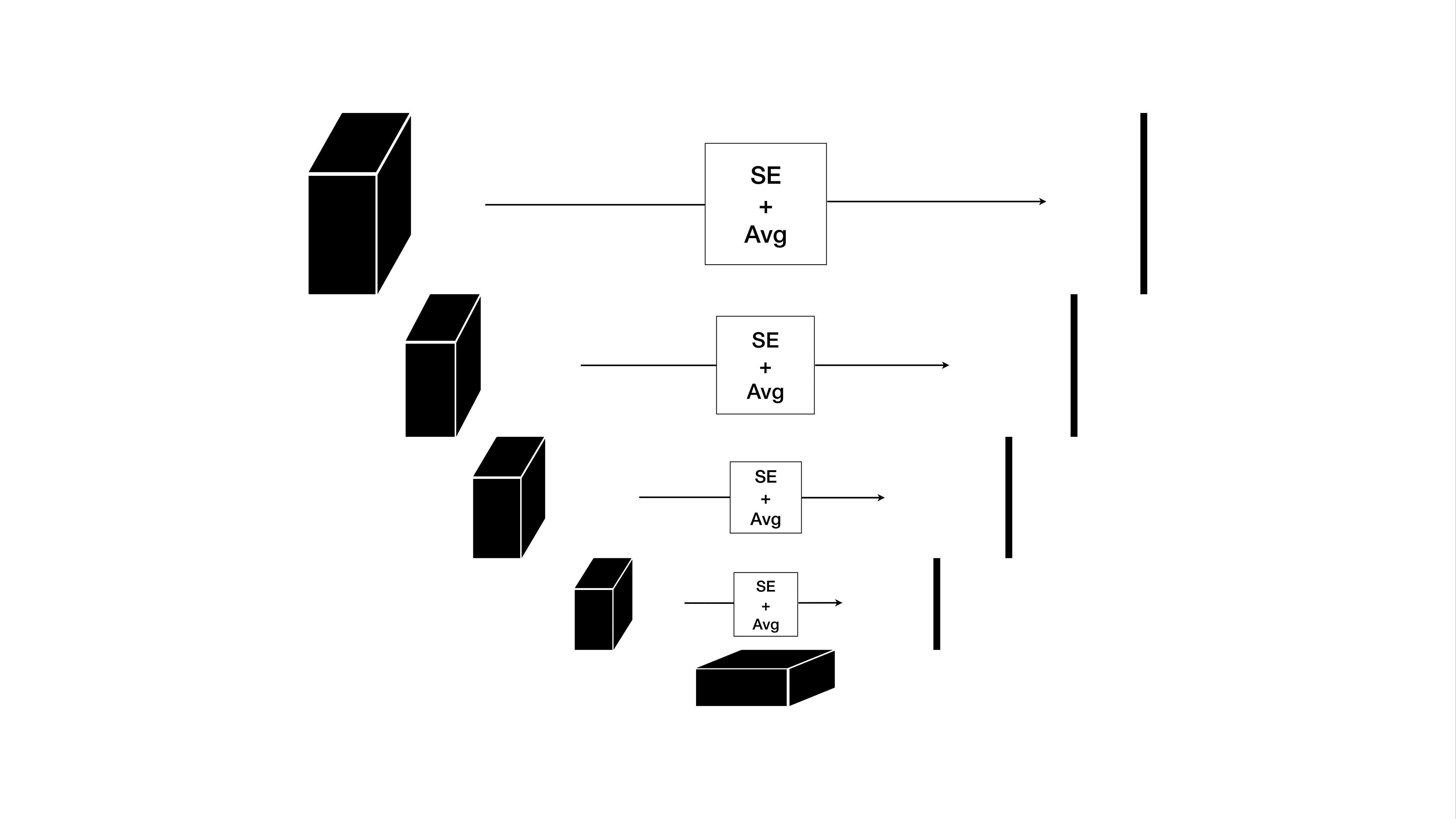\n\nAs been mentioned, we chose a 3D Encoder 2D Decoder U-Net model using SE blocks within the skip connections. Therefore, the selected slices were still seen as a 3D input volume by our network. After passing through the encoder, the features were mapped to 2D on all levels (i.e., skip connections) using a specific weighting. One unique aspect of the network to highlight is that the encoder contained four convolutions in each stage to process the difficult 3D input, whereas the decoder only had two convolutional blocks.\n\nThe mapping was initially performed using a simple average operation but was later refined with the use of Squeeze-and-Excitation. However, instead of applying the SE on the channel dimension — as is usually done to highlight important channels — we applied one SE Block per level (i.e., skip) to all channels, but on the x-dimension. This results in a weighting of the slices in feature space, so when aggregating with the average operation later, each slice has a different contribution.\n\n## Preprocessing\n\nIn the preprocessing stage, we cropped each fragment into 25 parts and ensured they contain an equal amount of data points (area labeled as foreground in the mask.png). This process was performed to create five folds for training.\n\nFor the selection of the 32 slices, we calculated the intensity distributions for each individual fragment. From these distributions, we determined the minimum and maximum values and calculated the middle point between them. We then cropped 32 slices around this chosen central slice. The following plot shows the intensity distribution for the individual fragments. The vertical line in the plot represents the midpoint between the maximum and minimum intensity values.\n\n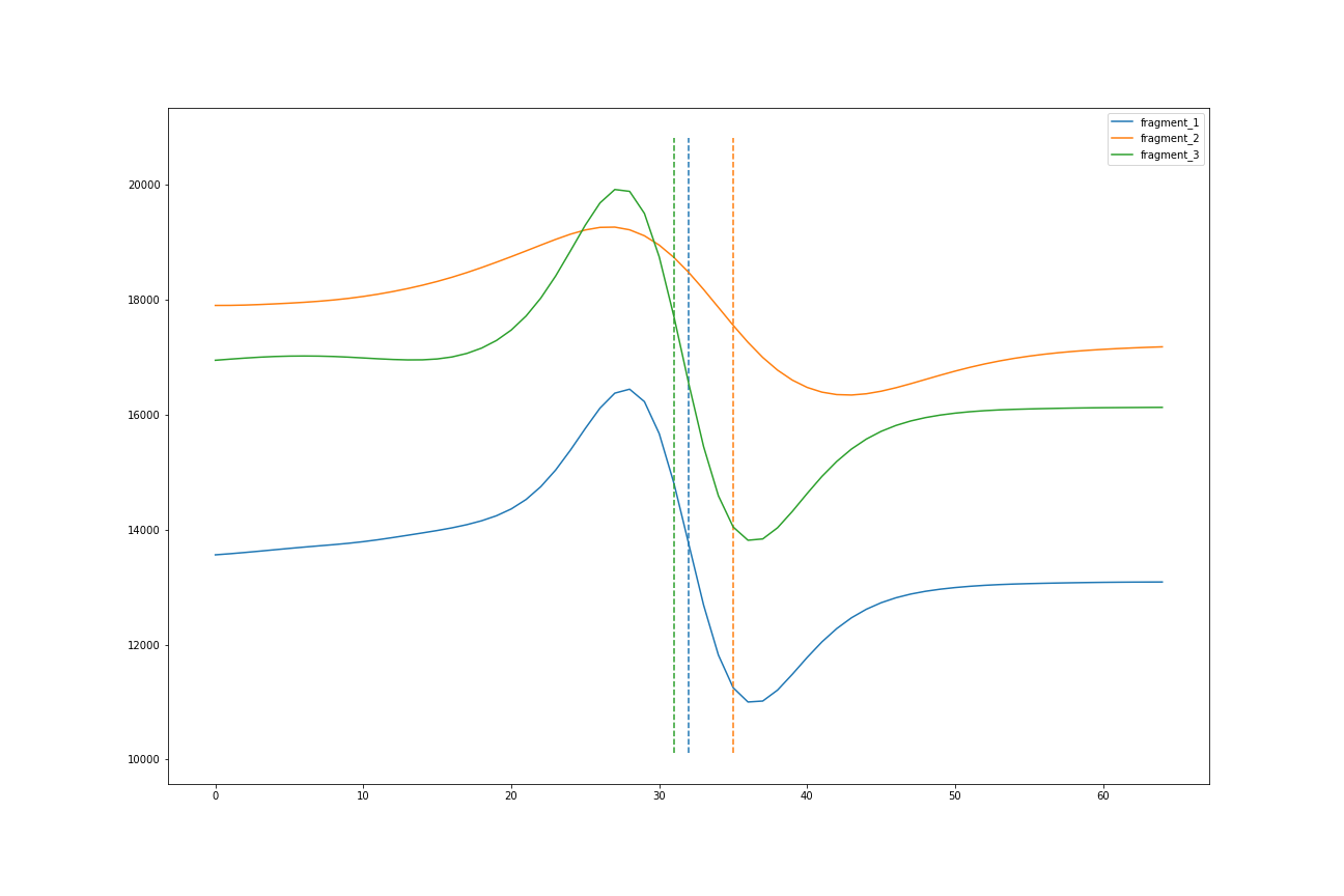\n\nTo further preprocess the data, we applied z-scoring to normalize the intensity values. Additionally, we clipped the intensity values at the 0.5 and 99.5 percentiles to remove extreme outliers. Finally, we performed normalization on each individual fragment to ensure consistency across the dataset.\n\n## Training\n\nHere are some insights into our training pipeline.\n\n### Augmentation\n\nFor the most part, we utilized the out-of-the-box augmentation techniques provided by nnU-Net, a framework specifically designed for medical image segmentation. These techniques formed the foundation of our data augmentation pipeline. However, we made certain modifications and additions to tailor the augmentation process to our specific task and data characteristics:\n\n- Rotation: We performed rotations only in the plane, meaning we applied rotations along the y and z axes. Out-of-plane rotations were considered as a measure to ensure stability but were not implemented.\n- Scaling: We introduced scaling augmentation, allowing the data to be randomly scaled within a certain range. This helped to increase the diversity of object sizes in the training data.\n- Gaussian Noise: We added Gaussian noise to the data, which helps to simulate realistic variations in image acquisition and improve the model's ability to handle noise.\n- Gaussian Blur: We applied Gaussian blur to the data, with varying levels of blurring intensity. This transformation aimed to capture the variations in image quality that can occur in different imaging settings.\n- Brightness and Contrast: We incorporated brightness and contrast augmentation to simulate variations in lighting conditions.\n- Simulate Low Resolution: We introduced a transformation to simulate low-resolution imaging by randomly zooming the data within a specified range. This augmentation aimed to make the model more robust to lower resolution images.\n- Gamma Transformation: We applied gamma transformations to the data, which adjusted the pixel intensities to enhance or reduce image contrast. This augmentation technique helps the model adapt to different contrast levels in input images.\n- Mirror Transform: We employed mirroring along specified axes to introduce further variations in object orientations and appearances.\n\n### Training Curves for Submission Folds\n\nBatch size of 4 and a weight decay of 1e-4. Fold 0.\n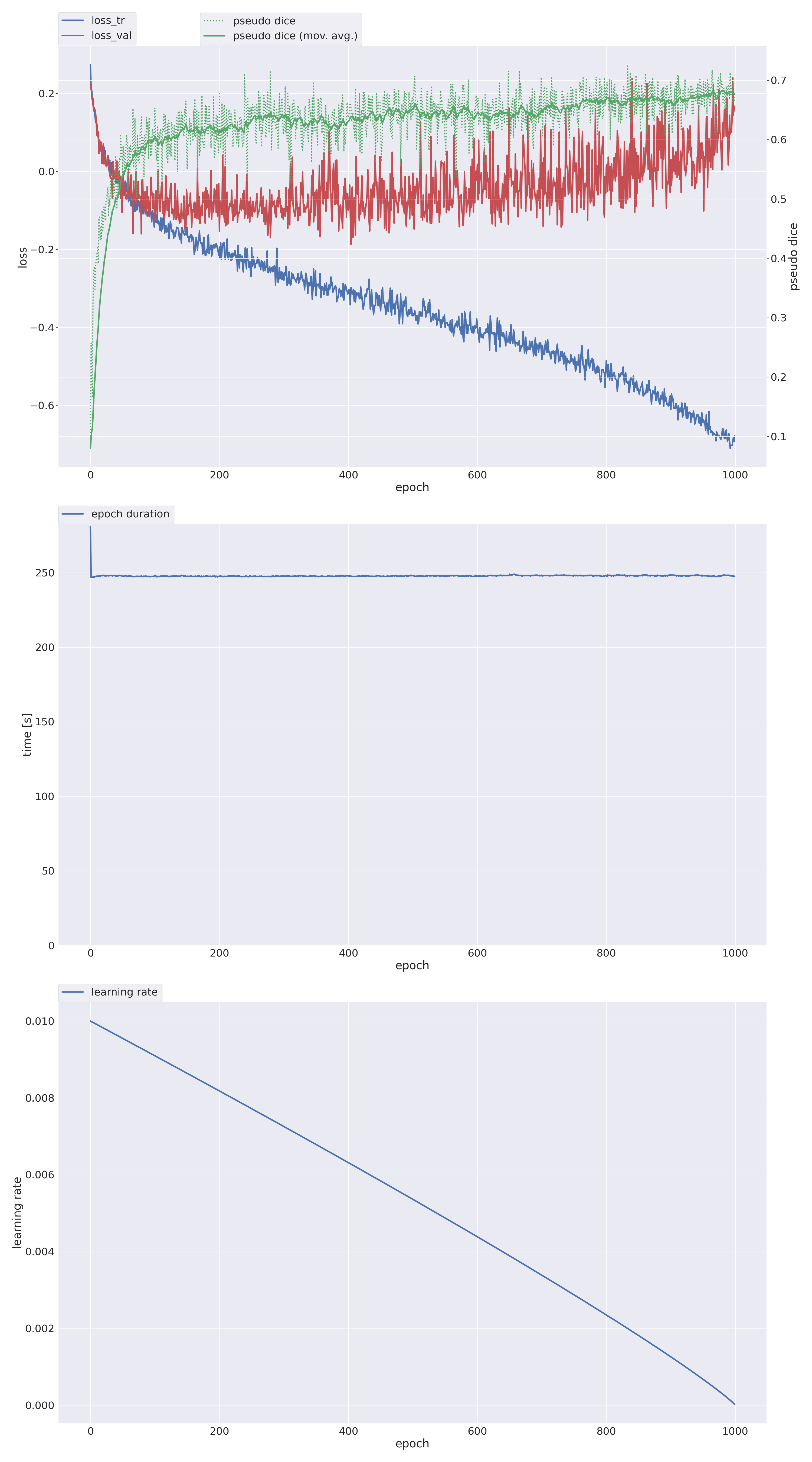\nBatch size of 4 and a weight decay of 1e-4. Fold 2.\n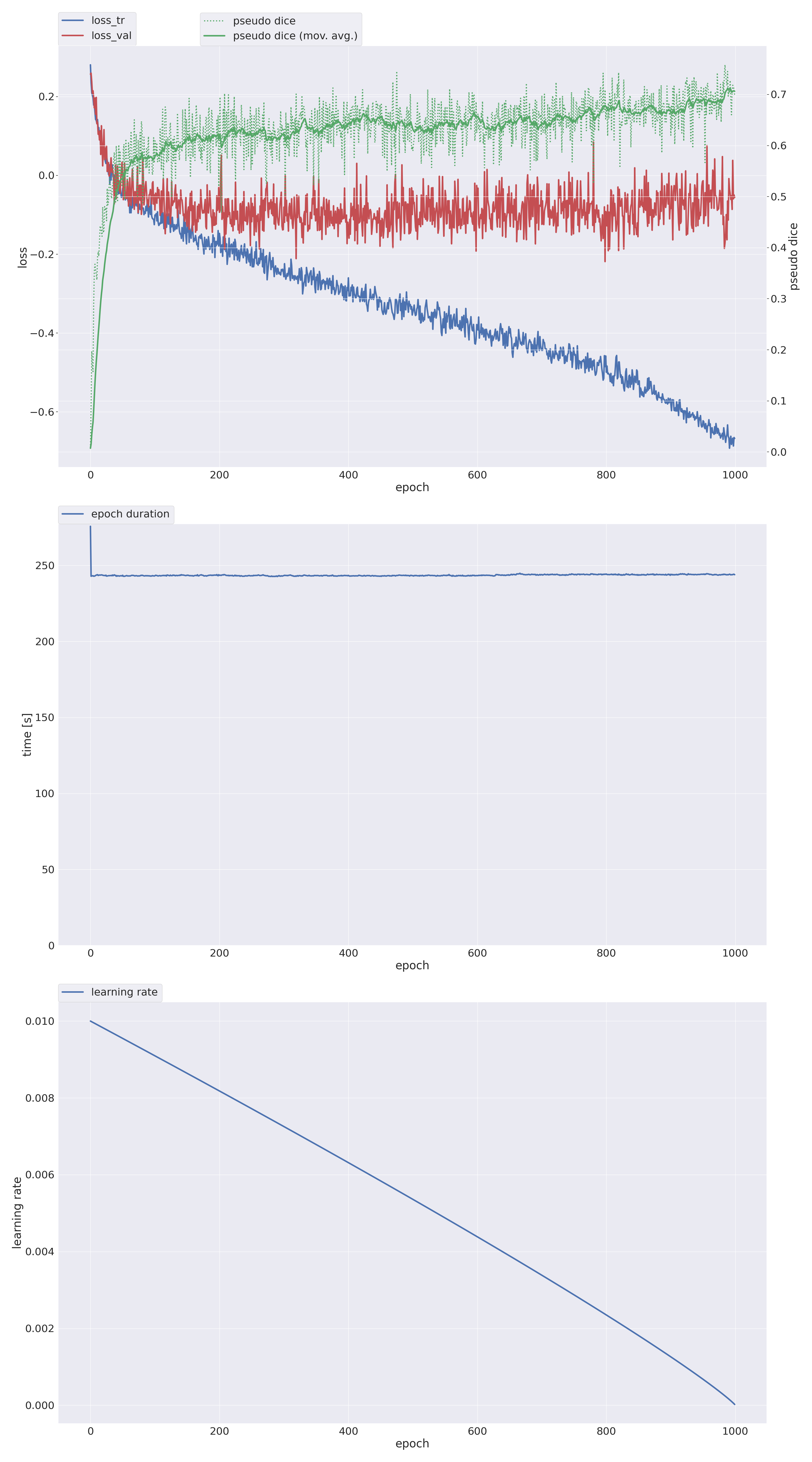\nBatch size of 2 and a weight decay of 3e-5. Fold 0.\n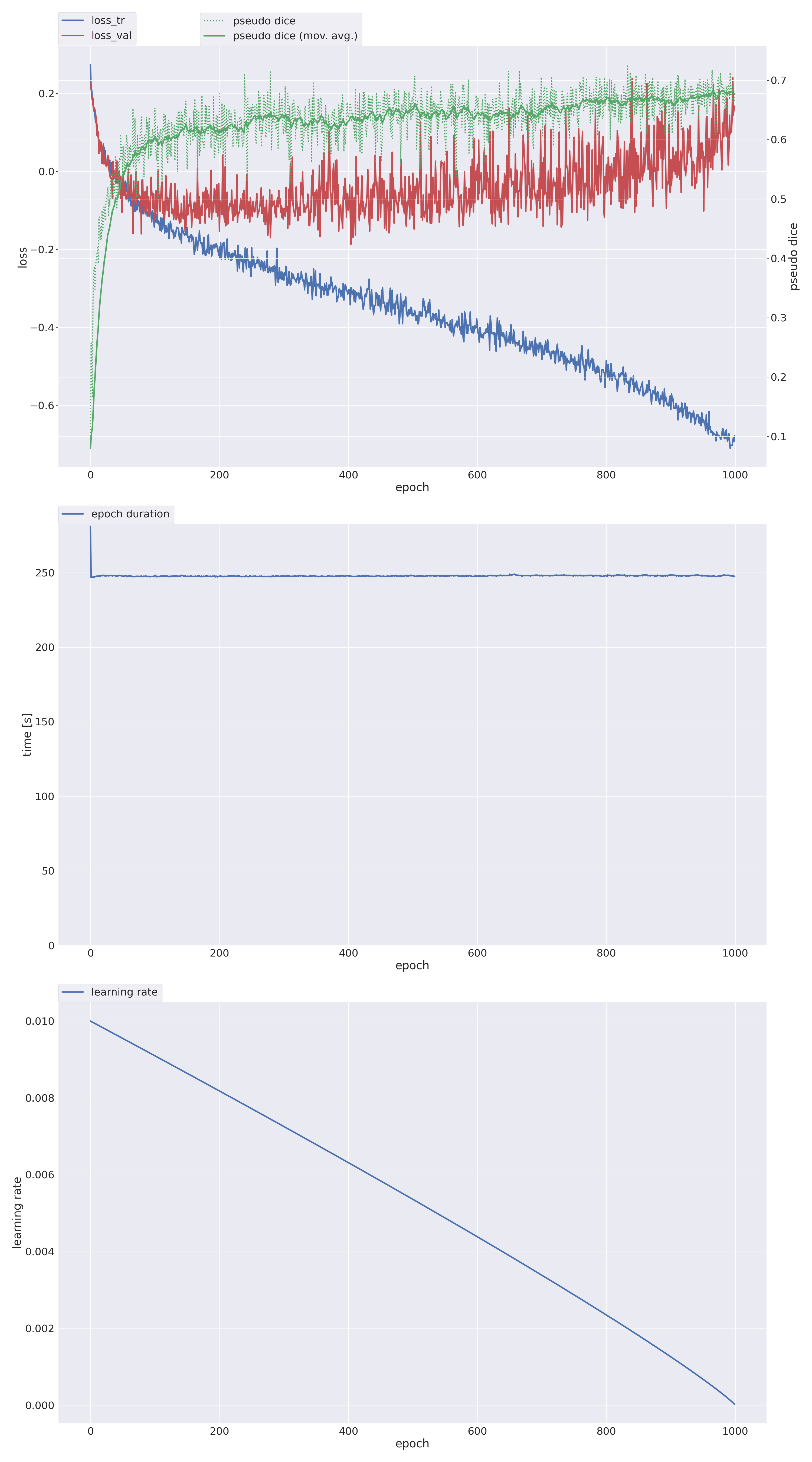\nBatch size of 2 and a weight decay of 3e-5. Fold 2.\n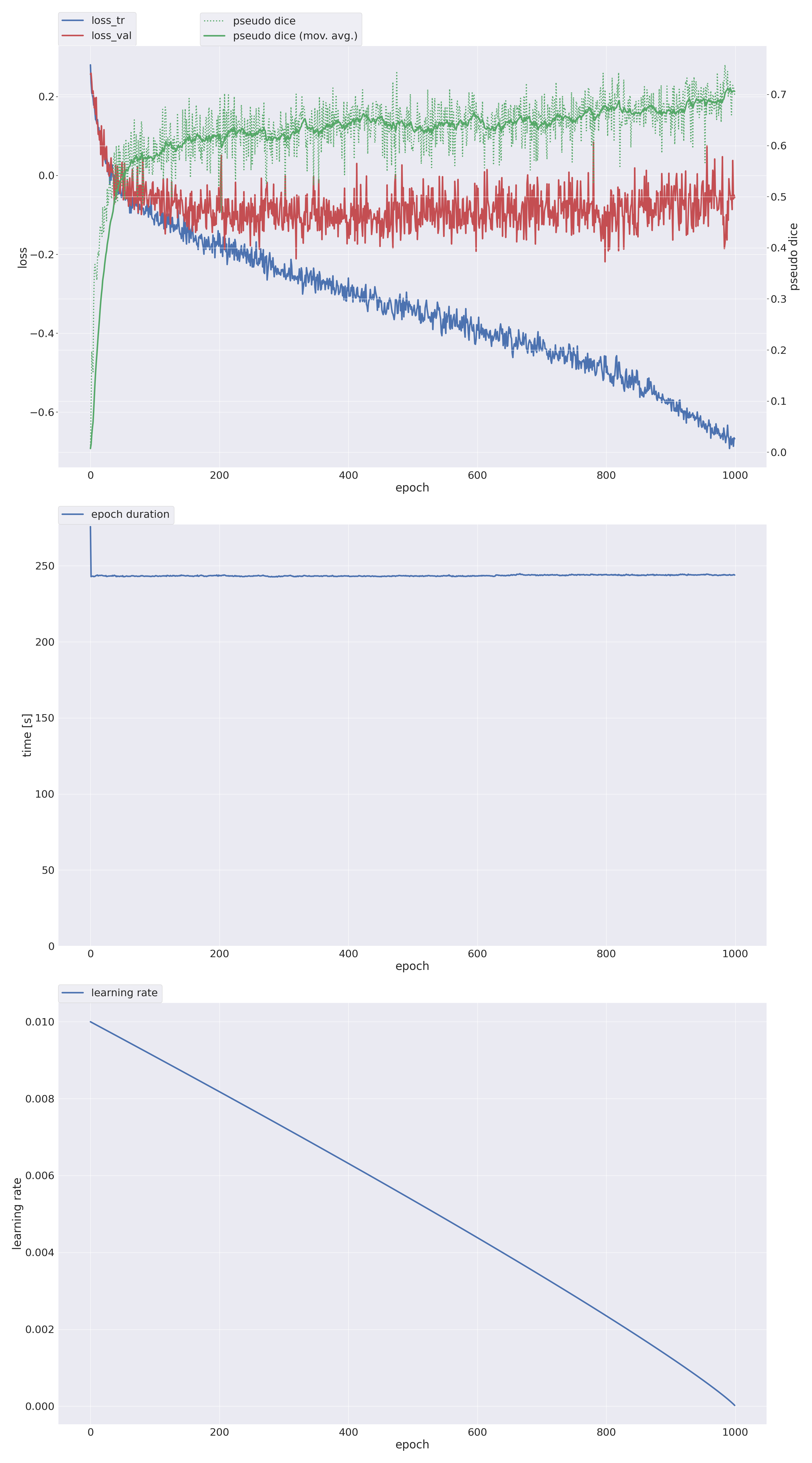\n\n## Inference\n\nWe made the decision to submit only the ensemble of fold 0 and fold 2 models due to their superior performance on the validation data compared to the other folds. The difference in Dice score between these two folds and the rest of the folds was substantial, with a margin of ~0.1. As a result, we deemed the ensemble of fold 0 and fold 2 models to be the most reliable and effective for our final submission (we fools).\n\nAdditionally, we made the decision to incorporate test time augmentation (TTA) techniques during the inference process. TTA involved applying mirroring along all axes and in-plane rotation of 90° to each patch. By performing these augmentations, we generated a total of eight separate predictions per model for each patch.\n\n### Post Processing\n\nIn a moment of desperate determination to achieve better results on the public test set, one audacious team member decided to dive headfirst into the realm of advanced post-processing. This daring soul concocted a daring plan: raise the threshold of the softmax outputs from a mundane 0.5 to a daring 0.6. But that was just the beginning!\n\nUndeterred by caution, the same intrepid individual embarked on a quest to conduct a connected component analysis, mercilessly discarding all instances with a lowly softmax 95th percentile value below the illustrious threshold of 0.8.\n\nWith fervor and a touch of madness, this brave adventurer tested countless combinations of thresholds, determined to find the golden ticket to enhanced validation scores across all folds. A relentless pursuit of validation improvement that knew no bounds.\n\nOn the public test set, this fearless undertaking delivered a substantial boost of 0.05 dice points, raising hopes and spirits across the team. The unexpected improvement injected a renewed sense of excitement and optimism.\n\nHowever, as fate would have it, on the ultimate battlefield of the 50% final, the outcome took a peculiar twist. The gains dwindled ever so slightly, with a meager decrease of -0.002 dice points. Though the difference may seem minuscule, in the realm of fierce competition, every decimal point counts.\n\nSorry guys.\n\n### 2D Unet Refinement \n\nThe second approach involved employing a 2D U-Net model with a patch size of 2048x2048 on the softmax outputs generated by the first model. Subsequently, the model's output was resized to 1024x1024 for inference purposes and then scaled up to the original resolution of 2048x2048. The rationale behind this strategy was to leverage the higher resolution input data to capture finer structural details, including the intricate shapes of letters. The training data for our this model was derived from inferences made by our various trained models on the original training data.\n\nWhose idea was this?\n\nSorry again.\n\n## Preliminary Last Words\n\nMore details and code will follow, cheers!", "votes": 30 }, { "id": 2306303, "postDate": "2023-06-17T07:51:28.517Z", "content": "A very enjoyable write up! Your \"group of PhD students from the lab where nnUNet was developed\" and witty writing talents - sounds like a pilot for The Big Scroll.
\nCongrats to your team and the intrepid adventurer.
Wherever this daring wonderer of a post processing legend remains today - he may rest in peace and all his desperate tries of utter panic to increase the score shall be forgiven. Someday he will properly possess the power to post process - but until this day we will remain calm and only feel love for his poor soul. He had no chance of knowing better <3
", "rawMarkdown": "Wherever this daring wonderer of a post processing legend remains today - he may rest in peace and all his desperate tries of utter panic to increase the score shall be forgiven. Someday he will properly possess the power to post process - but until this day we will remain calm and only feel love for his poor soul. He had no chance of knowing better <3", "votes": 3 }, { "id": 2304175, "postDate": "2023-06-15T18:32:15.197Z", "content": "Lots of love for this unknown adventurer who tried his best to push our results even further - and nearly succeeded. Let's see what the final results will show.
", "rawMarkdown": "Lots of love for this unknown adventurer who tried his best to push our results even further - and nearly succeeded. Let's see what the final results will show.", "votes": 3 }, { "id": 2304438, "postDate": "2023-06-16T02:07:52.997Z", "content": "Just realizing the labels on the graphs. did you actually train for 1000 epochs?
", "rawMarkdown": "Just realizing the labels on the graphs. did you actually train for 1000 epochs?", "votes": 1, "replies": [ { "id": 2304745, "postDate": "2023-06-16T07:52:36.157Z", "rawMarkdown": "", "isDeleted": true }, { "id": 2304750, "postDate": "2023-06-16T07:56:05.763Z", "content": "Yes, we tried different schedules but this combination of optimizer, learning rate scheduler and number of training epochs yielded the best end results on our validation splits and also on the leaderboard. For some configurations which didn't make it into the final choice 2000 epochs worked even better than 1000, even though the models already go into slight overfitting after ~150 epochs.
", "rawMarkdown": "Yes, we tried different schedules but this combination of optimizer, learning rate scheduler and number of training epochs yielded the best end results on our validation splits and also on the leaderboard. For some configurations which didn't make it into the final choice 2000 epochs worked even better than 1000, even though the models already go into slight overfitting after ~150 epochs.", "votes": 1 }, { "id": 2304766, "postDate": "2023-06-16T08:10:05.923Z", "content": "Yes, but we primarily evaluated the model with the best EMA pseudo Dice score, in addition to the final model. Usually, the best EMA pseudo Dice model performed the best.
", "rawMarkdown": "Yes, but we primarily evaluated the model with the best EMA pseudo Dice score, in addition to the final model. Usually, the best EMA pseudo Dice model performed the best." } ] }, { "id": 2304381, "postDate": "2023-06-16T00:45:58.180Z", "content": "Very interesting that you used nnU-net. I looked all around at various medical imaging models and didnt see that one. I was mostly looking at unetr and unetr++ and nnformer, but I never got around to trying all of them. How did you come across nnU-net?
", "rawMarkdown": "Very interesting that you used nnU-net. I looked all around at various medical imaging models and didnt see that one. I was mostly looking at unetr and unetr++ and nnformer, but I never got around to trying all of them. How did you come across nnU-net?", "votes": 2, "replies": [ { "id": 2304742, "postDate": "2023-06-16T07:51:07.950Z", "content": "We are a group of PhD students from the lab where nnUNet was developed, so it was a natural choice for us to use it as the underlying framework. The neat thing about nnUNet is that it already takes care of many things out of the box and is highly optimized for that. Therefore you can just work on what you need for your specific task. In the case of this challenge that meant modifying nearly every part of the pipeline from preprocessing, the used architecture, inference and postprocessing. You can also quite easily add architectures that are not standard UNet based like the mentioned UNetr or also SwinUNetr but in this very low data regime we figured that the inductive bias of convolutional networks would be beneficient for our training. We plan to publish our full code with modifications of the nnUNet in a repo which we will link here. If you are interested you can have a look to see how you can use and modify nnUNet yourself.
", "rawMarkdown": "We are a group of PhD students from the lab where nnUNet was developed, so it was a natural choice for us to use it as the underlying framework. The neat thing about nnUNet is that it already takes care of many things out of the box and is highly optimized for that. Therefore you can just work on what you need for your specific task. In the case of this challenge that meant modifying nearly every part of the pipeline from preprocessing, the used architecture, inference and postprocessing. You can also quite easily add architectures that are not standard UNet based like the mentioned UNetr or also SwinUNetr but in this very low data regime we figured that the inductive bias of convolutional networks would be beneficient for our training. We plan to publish our full code with modifications of the nnUNet in a repo which we will link here. If you are interested you can have a look to see how you can use and modify nnUNet yourself.", "votes": 4, "replies": [ { "id": 2305471, "postDate": "2023-06-16T17:59:35.077Z", "content": "Thank you for sharing. This sounds great, and I look forward to checking out nnUNet.
", "rawMarkdown": "Thank you for sharing. This sounds great, and I look forward to checking out nnUNet.", "votes": 2 }, { "id": 2308042, "postDate": "2023-06-18T16:06:09.523Z", "content": "That's very interesting. Is there an open-source implementation of nnU-Net? You are probably referring to this one => https://github.com/MIC-DKFZ/nnUNet
", "rawMarkdown": "That's very interesting. Is there an open-source implementation of nnU-Net? You are probably referring to this one => https://github.com/MIC-DKFZ/nnUNet" }, { "id": 2308067, "postDate": "2023-06-18T16:30:15Z", "content": "Thank you! Yes exactly, there is the official GitHub repo of nnUNet which you linked and our challenge code with all the modifications is now also available at https://github.com/MIC-DKFZ/OverthINKingSegmenter
", "rawMarkdown": "Thank you! Yes exactly, there is the official GitHub repo of nnUNet which you linked and our challenge code with all the modifications is now also available at https://github.com/MIC-DKFZ/OverthINKingSegmenter", "votes": 3 }, { "id": 2309087, "postDate": "2023-06-19T11:45:38.667Z", "content": "That's great, thanks for sharing!
", "rawMarkdown": "That's great, thanks for sharing! " } ] } ] }, { "id": 2308039, "postDate": "2023-06-18T16:03:46.280Z", "content": "Very nice write-up. The graph to choose the slices is a good idea. Plus a lot of nice monitoring graphs, thanks for sharing!
", "rawMarkdown": "Very nice write-up. The graph to choose the slices is a good idea. Plus a lot of nice monitoring graphs, thanks for sharing!", "replies": [ { "id": 2308075, "postDate": "2023-06-18T16:32:10.583Z", "content": "Thank you!
", "rawMarkdown": "Thank you!" } ] } ], "comments": [ { "id": 2306303, "author_name": "something4kag", "author_url": "", "post_date": "2023-06-17T07:51:28.517000", "content": "A very enjoyable write up! Your \"group of PhD students from the lab where nnUNet was developed\" and witty writing talents - sounds like a pilot for The Big Scroll.
\nCongrats to your team and the intrepid adventurer.
Wherever this daring wonderer of a post processing legend remains today - he may rest in peace and all his desperate tries of utter panic to increase the score shall be forgiven. Someday he will properly possess the power to post process - but until this day we will remain calm and only feel love for his poor soul. He had no chance of knowing better <3
", "votes": 3, "replies": [] }, { "id": 2304175, "author_name": "YanKir", "author_url": "", "post_date": "2023-06-15T18:32:15.197000", "content": "Lots of love for this unknown adventurer who tried his best to push our results even further - and nearly succeeded. Let's see what the final results will show.
", "votes": 3, "replies": [] }, { "id": 2304438, "author_name": "ryches", "author_url": "", "post_date": "2023-06-16T02:07:52.997000", "content": "Just realizing the labels on the graphs. did you actually train for 1000 epochs?
", "votes": 1, "replies": [ { "id": 2304745, "author_name": "", "author_url": "", "post_date": "2023-06-16T07:52:36.157000", "content": "", "votes": 0, "replies": [] }, { "id": 2304750, "author_name": "YanKir", "author_url": "", "post_date": "2023-06-16T07:56:05.763000", "content": "Yes, we tried different schedules but this combination of optimizer, learning rate scheduler and number of training epochs yielded the best end results on our validation splits and also on the leaderboard. For some configurations which didn't make it into the final choice 2000 epochs worked even better than 1000, even though the models already go into slight overfitting after ~150 epochs.
", "votes": 1, "replies": [] }, { "id": 2304766, "author_name": "Benjamin Hamm", "author_url": "", "post_date": "2023-06-16T08:10:05.923000", "content": "Yes, but we primarily evaluated the model with the best EMA pseudo Dice score, in addition to the final model. Usually, the best EMA pseudo Dice model performed the best.
", "votes": 0, "replies": [] } ] }, { "id": 2304381, "author_name": "ryches", "author_url": "", "post_date": "2023-06-16T00:45:58.180000", "content": "Very interesting that you used nnU-net. I looked all around at various medical imaging models and didnt see that one. I was mostly looking at unetr and unetr++ and nnformer, but I never got around to trying all of them. How did you come across nnU-net?
", "votes": 2, "replies": [ { "id": 2304742, "author_name": "YanKir", "author_url": "", "post_date": "2023-06-16T07:51:07.950000", "content": "We are a group of PhD students from the lab where nnUNet was developed, so it was a natural choice for us to use it as the underlying framework. The neat thing about nnUNet is that it already takes care of many things out of the box and is highly optimized for that. Therefore you can just work on what you need for your specific task. In the case of this challenge that meant modifying nearly every part of the pipeline from preprocessing, the used architecture, inference and postprocessing. You can also quite easily add architectures that are not standard UNet based like the mentioned UNetr or also SwinUNetr but in this very low data regime we figured that the inductive bias of convolutional networks would be beneficient for our training. We plan to publish our full code with modifications of the nnUNet in a repo which we will link here. If you are interested you can have a look to see how you can use and modify nnUNet yourself.
", "votes": 4, "replies": [ { "id": 2305471, "author_name": "Ted K", "author_url": "", "post_date": "2023-06-16T17:59:35.077000", "content": "Thank you for sharing. This sounds great, and I look forward to checking out nnUNet.
", "votes": 2, "replies": [] }, { "id": 2308042, "author_name": "Yassine Alouini", "author_url": "", "post_date": "2023-06-18T16:06:09.523000", "content": "That's very interesting. Is there an open-source implementation of nnU-Net? You are probably referring to this one => https://github.com/MIC-DKFZ/nnUNet
", "votes": 0, "replies": [] }, { "id": 2308067, "author_name": "YanKir", "author_url": "", "post_date": "2023-06-18T16:30:15", "content": "Thank you! Yes exactly, there is the official GitHub repo of nnUNet which you linked and our challenge code with all the modifications is now also available at https://github.com/MIC-DKFZ/OverthINKingSegmenter
", "votes": 3, "replies": [] }, { "id": 2309087, "author_name": "Yassine Alouini", "author_url": "", "post_date": "2023-06-19T11:45:38.667000", "content": "That's great, thanks for sharing!
", "votes": 0, "replies": [] } ] } ] }, { "id": 2308039, "author_name": "Yassine Alouini", "author_url": "", "post_date": "2023-06-18T16:03:46.280000", "content": "Very nice write-up. The graph to choose the slices is a good idea. Plus a lot of nice monitoring graphs, thanks for sharing!
", "votes": 0, "replies": [ { "id": 2308075, "author_name": "YanKir", "author_url": "", "post_date": "2023-06-18T16:32:10.583000", "content": "Thank you!
", "votes": 0, "replies": [] } ] } ], "raw_markdown_by_id": { "2304075": "We are very grateful for the organization of this very interesting competition. Sincere thanks to the hosts and the Kaggle team. A big thank you to Yannick and Max, it was lots of fun working with you! For all of us it was the first Kaggle competition. \n\n## Summary\n\nIn this competition submission, we used the [nnU-Net framework](https://github.com/MIC-DKFZ/nnUNet), a recognized powerhouse in the medical imaging domain. The success of nnU-Net is validated by its adoption in winning solutions of 9 out of 10 challenges at [MICCAI 2020](https://arxiv.org/abs/2101.00232), 5 out of 7 in MICCAI 2021 and the first place in the [AMOS 2022](https://amos22.grand-challenge.org/final-ranking/) challange.\n\nTo tackle the three-dimensional nature of the given task, we designed a custom network architecture: a 3D Encoder 2D Decoder U-Net model using Squeeze-and-Excitation (SE) blocks within the skip connections. We used fragment-wise normalization and selected 32 slices for training, enabling us to extend the patch size to 32x512x512. We divided each fragment into 25 pieces and trained five folds. We only submitted models that performed well on our validation data. For the final submission, we ensambled the weights of two folds (zero and two) from two respective models. One model was trained with a batch size of 2 and a weight decay of 3e-5, while the other was trained with a batch size of 4 and a weight decay of 1e-4. During test time augmentation, we implemented mirroring along all axes and in-plane rotation of 90°, resulting in a total of eight separate predictions per model for each patch. \n\nFor the two submissions we chose two different postprcessing techniques. The first approach involved setting the threshold of the softmax outputs from the network from 0.5 to 0.6. As a second step we conducted a connected component analysis to eliminate all instances with a softmax 95th percentile value below 0.8. The second approach involved utilizing an off-the-shelf 2D U-Net model with a patch size of 2048x2048 on the softmax outputs of the first model. The output was resized to 1024x1024 for inference and then scaled up to 2048x2048. The intention behind this step was to capture more structural elements, such as the shape of letters, due to the higher resolution of the input. We regret both since they only improved results for public testset.\n\n## Model Architecture\n\n\n\nAs been mentioned, we chose a 3D Encoder 2D Decoder U-Net model using SE blocks within the skip connections. Therefore, the selected slices were still seen as a 3D input volume by our network. After passing through the encoder, the features were mapped to 2D on all levels (i.e., skip connections) using a specific weighting. One unique aspect of the network to highlight is that the encoder contained four convolutions in each stage to process the difficult 3D input, whereas the decoder only had two convolutional blocks.\n\nThe mapping was initially performed using a simple average operation but was later refined with the use of Squeeze-and-Excitation. However, instead of applying the SE on the channel dimension — as is usually done to highlight important channels — we applied one SE Block per level (i.e., skip) to all channels, but on the x-dimension. This results in a weighting of the slices in feature space, so when aggregating with the average operation later, each slice has a different contribution.\n\n## Preprocessing\n\nIn the preprocessing stage, we cropped each fragment into 25 parts and ensured they contain an equal amount of data points (area labeled as foreground in the mask.png). This process was performed to create five folds for training.\n\nFor the selection of the 32 slices, we calculated the intensity distributions for each individual fragment. From these distributions, we determined the minimum and maximum values and calculated the middle point between them. We then cropped 32 slices around this chosen central slice. The following plot shows the intensity distribution for the individual fragments. The vertical line in the plot represents the midpoint between the maximum and minimum intensity values.\n\n\n\nTo further preprocess the data, we applied z-scoring to normalize the intensity values. Additionally, we clipped the intensity values at the 0.5 and 99.5 percentiles to remove extreme outliers. Finally, we performed normalization on each individual fragment to ensure consistency across the dataset.\n\n## Training\n\nHere are some insights into our training pipeline.\n\n### Augmentation\n\nFor the most part, we utilized the out-of-the-box augmentation techniques provided by nnU-Net, a framework specifically designed for medical image segmentation. These techniques formed the foundation of our data augmentation pipeline. However, we made certain modifications and additions to tailor the augmentation process to our specific task and data characteristics:\n\n- Rotation: We performed rotations only in the plane, meaning we applied rotations along the y and z axes. Out-of-plane rotations were considered as a measure to ensure stability but were not implemented.\n- Scaling: We introduced scaling augmentation, allowing the data to be randomly scaled within a certain range. This helped to increase the diversity of object sizes in the training data.\n- Gaussian Noise: We added Gaussian noise to the data, which helps to simulate realistic variations in image acquisition and improve the model's ability to handle noise.\n- Gaussian Blur: We applied Gaussian blur to the data, with varying levels of blurring intensity. This transformation aimed to capture the variations in image quality that can occur in different imaging settings.\n- Brightness and Contrast: We incorporated brightness and contrast augmentation to simulate variations in lighting conditions.\n- Simulate Low Resolution: We introduced a transformation to simulate low-resolution imaging by randomly zooming the data within a specified range. This augmentation aimed to make the model more robust to lower resolution images.\n- Gamma Transformation: We applied gamma transformations to the data, which adjusted the pixel intensities to enhance or reduce image contrast. This augmentation technique helps the model adapt to different contrast levels in input images.\n- Mirror Transform: We employed mirroring along specified axes to introduce further variations in object orientations and appearances.\n\n### Training Curves for Submission Folds\n\nBatch size of 4 and a weight decay of 1e-4. Fold 0.\n\nBatch size of 4 and a weight decay of 1e-4. Fold 2.\n\nBatch size of 2 and a weight decay of 3e-5. Fold 0.\n\nBatch size of 2 and a weight decay of 3e-5. Fold 2.\n\n\n## Inference\n\nWe made the decision to submit only the ensemble of fold 0 and fold 2 models due to their superior performance on the validation data compared to the other folds. The difference in Dice score between these two folds and the rest of the folds was substantial, with a margin of ~0.1. As a result, we deemed the ensemble of fold 0 and fold 2 models to be the most reliable and effective for our final submission (we fools).\n\nAdditionally, we made the decision to incorporate test time augmentation (TTA) techniques during the inference process. TTA involved applying mirroring along all axes and in-plane rotation of 90° to each patch. By performing these augmentations, we generated a total of eight separate predictions per model for each patch.\n\n### Post Processing\n\nIn a moment of desperate determination to achieve better results on the public test set, one audacious team member decided to dive headfirst into the realm of advanced post-processing. This daring soul concocted a daring plan: raise the threshold of the softmax outputs from a mundane 0.5 to a daring 0.6. But that was just the beginning!\n\nUndeterred by caution, the same intrepid individual embarked on a quest to conduct a connected component analysis, mercilessly discarding all instances with a lowly softmax 95th percentile value below the illustrious threshold of 0.8.\n\nWith fervor and a touch of madness, this brave adventurer tested countless combinations of thresholds, determined to find the golden ticket to enhanced validation scores across all folds. A relentless pursuit of validation improvement that knew no bounds.\n\nOn the public test set, this fearless undertaking delivered a substantial boost of 0.05 dice points, raising hopes and spirits across the team. The unexpected improvement injected a renewed sense of excitement and optimism.\n\nHowever, as fate would have it, on the ultimate battlefield of the 50% final, the outcome took a peculiar twist. The gains dwindled ever so slightly, with a meager decrease of -0.002 dice points. Though the difference may seem minuscule, in the realm of fierce competition, every decimal point counts.\n\nSorry guys.\n\n### 2D Unet Refinement \n\nThe second approach involved employing a 2D U-Net model with a patch size of 2048x2048 on the softmax outputs generated by the first model. Subsequently, the model's output was resized to 1024x1024 for inference purposes and then scaled up to the original resolution of 2048x2048. The rationale behind this strategy was to leverage the higher resolution input data to capture finer structural details, including the intricate shapes of letters. The training data for our this model was derived from inferences made by our various trained models on the original training data.\n\nWhose idea was this?\n\nSorry again.\n\n## Preliminary Last Words\n\nMore details and code will follow, cheers!", "2306303": "A very enjoyable write up! Your \"group of PhD students from the lab where nnUNet was developed\" and witty writing talents - sounds like a pilot for The Big Scroll. \nCongrats to your team and the intrepid adventurer. ", "2304288": "Wherever this daring wonderer of a post processing legend remains today - he may rest in peace and all his desperate tries of utter panic to increase the score shall be forgiven. Someday he will properly possess the power to post process - but until this day we will remain calm and only feel love for his poor soul. He had no chance of knowing better <3", "2304175": "Lots of love for this unknown adventurer who tried his best to push our results even further - and nearly succeeded. Let's see what the final results will show.", "2304438": "Just realizing the labels on the graphs. did you actually train for 1000 epochs?", "2304381": "Very interesting that you used nnU-net. I looked all around at various medical imaging models and didnt see that one. I was mostly looking at unetr and unetr++ and nnformer, but I never got around to trying all of them. How did you come across nnU-net?", "2308039": "Very nice write-up. The graph to choose the slices is a good idea. Plus a lot of nice monitoring graphs, thanks for sharing!" } }