---
title: "A Beginner's Guide to CERN's TrackML Challenge"
author: "Pranav Pandya"
output:
html_document:
number_sections: false
code_folding: show
toc: true
toc_depth: 6
fig_width: 10
highlight: tango
theme: cosmo
smart: true
editor_options:
chunk_output_type: console
---
-------------------------------------------------------------------------------------
**update** : Added simple approach to calculate EPS value (part 3)
# Introduction
To explore what our universe is made of, scientists at CERN are colliding protons, essentially recreating mini big bangs, and meticulously observing these collisions with intricate silicon detectors. While orchestrating the collisions and observations is already a massive scientific accomplishment, analyzing the enormous amounts of data produced from the experiments is becoming an overwhelming challenge.
In this challenge, a team of Machine Learning experts and physics scientists working at CERN (the world largest high energy physics laboratory), has partnered with Kaggle and prestigious sponsors to answer the question:
**can machine learning assist high energy physics in discovering and characterizing new particles?**
## What is Particle physics?
* Particle physics is the study of subatomic particles and the fundamental forces that act between them.
* Present-day particle physics research represents man’s most ambitious and organised effort to answer the question: What is the universe made of?
* Just to give you an idea, Higgs boson was found after a 40-year search.
## Particle physics and The Large Hadron Collider (LHC)
To find the Higgs boson and attempt to unlock some other mysteries, CERN needed to:
* Build the world’s most powerful particle accelerator and largest machine (LHC) ever constructed by humankind
* Construct incredibly sophisticated particle detectors
* Collect an enormous amount of data
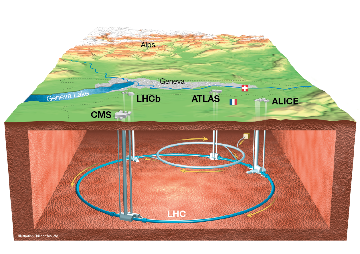
Note: ATLAS, ALICE, CMS and LHCb [refers](https://universe-review.ca/R15-20-accelerators03.htm) to name of detectors
* ALICE: A Large Ion Collider Experiment
* ATLAS: A large Toroidal LHC ApparatuS
* CMS : Compact Muon Solenoid
* LHCb : Large Hadron Collider beauty
Let's get started with exploratory data analysis to see how the data looks like.
# Part 1: Data Exploration
In this part, we will explore the data for **single event** to get a quick overview. Each event contains simulated measurements (essentially 3D points) of particles generated in a collision between proton bunches at the [Large Hadron Collider](https://home.cern/topics/large-hadron-collider) at [CERN](https://home.cern).
The training dataset contains the recorded hits, their ground truth counterpart and their association to particles, and the initial parameters of those particles. The test dataset contains only the recorded hits.
-------------------------------------------------------------------------------------
## Extract data for event000001000
```{r message=FALSE}
if (!require("pacman")) install.packages("pacman")
pacman::p_load(knitr, tidyverse, highcharter, data.table, tictoc, DT, viridis, plotly, DescTools, fpc, dbscan, factoextra)
options(warn = -1)
event000001000 <- lapply(Sys.glob("../input/train_1/event000001000*.csv"), fread)
str(event000001000, max=1)
```
There are 4 files within selected event. Let's extract each file one by one. In the following sections, initial tab contains glimpse of each table and other tabs contains distribution information of important variables.
### Event hits {.tabset .tabset-fade .tabset-pills}
The hits file contains the following values for each hit/entry:
* **hit_id**: numerical identifier of the hit inside the event.
* **x, y, z**: measured x, y, z position (in millimeter) of the hit in global coordinates.
* **volume_id**: numerical identifier of the detector group.
* **layer_id**: numerical identifier of the detector layer inside the group.
* **module_id**: numerical identifier of the detector module inside the layer.
The volume/layer/module id could in principle be deduced from x, y, z. They are given here to simplify detector-specific data handling.
#### Glimpse
```{r message=FALSE}
hits <- as.data.frame(event000001000[2])
head(hits, 10) %>%
datatable(style="bootstrap", options = list(dom = 'tp', pageLength = 5))
```
**Unique values by each variable in hits**
```{r message=FALSE}
kable(as.data.frame(lapply(hits, function(x)length(unique(x)))))
```
#### X coordinate
```{r message=FALSE}
PlotFdist(hits$x, "Distribution of X co-ord position")
```
#### Y coordinate
```{r message=FALSE}
PlotFdist(hits$y, "Distribution of Y co-ord position")
```
#### Zcoordinate
```{r message=FALSE}
PlotFdist(hits$z, "Distribution of Z co-ord position")
```
### Event cells {.tabset .tabset-fade .tabset-pills}
The cells file contains the constituent active detector cells that comprise each hit.
* **hit_id**: numerical identifier of the hit as defined in the hits file.
* **ch0, ch1**: channel identifier/coordinates unique within one module.
* **value**: signal value information, e.g. how much charge a particle has deposited.
#### Glimpse
```{r message=FALSE}
cells <- as.data.frame(event000001000[1])
head(cells, 10) %>%
datatable(style="bootstrap", options = list(dom = 'tp', pageLength = 5))
```
**Unique values by each variable in Cells**
```{r message=FALSE}
kable(as.data.frame(lapply(cells, function(x)length(unique(x)))))
```
#### Value of charge deposited by particle
```{r message=FALSE}
PlotFdist(cells$value, "Distribution of charge deposited by particle")
```
### Event particles {.tabset .tabset-fade .tabset-pills}
The particles files contains the following values for each particle/entry:
* **particle_id**: numerical identifier of the particle inside the event.
* **vx, vy, vz**: initial position or vertex (in millimeters) in global coordinates.
* **px, py, pz**: initial momentum (in GeV/c) along each global axis.
* **q**: particle charge (as multiple of the absolute electron charge).
* **nhits**: number of hits generated by this particle.
All entries contain the generated information or ground truth.
#### Glimpse
```{r message=FALSE}
particles <- as.data.frame(event000001000[3])
head(particles, 10) %>%
datatable(style="bootstrap", options = list(dom = 'tp', pageLength = 5))
```
**Unique values by each variable in Particles file**
```{r message=FALSE}
kable(as.data.frame(lapply(particles, function(x)length(unique(x)))))
```
#### Vertex {.tabset .tabset-fade .tabset-pills}
##### vx
```{r message=FALSE}
PlotFdist(particles$vx)
```
##### vy
```{r message=FALSE}
PlotFdist(particles$vy)
```
##### vz
```{r message=FALSE}
PlotFdist(particles$vz)
```
#### Initial momentum {.tabset .tabset-fade .tabset-pills}
##### px
```{r message=FALSE}
PlotFdist(particles$px)
```
##### py
```{r message=FALSE}
PlotFdist(particles$py)
```
##### pz
```{r message=FALSE}
PlotFdist(particles$pz)
```
#### Number of hits by particle
```{r message=FALSE}
PlotFdist(particles$nhits)
```
### Event truth {.tabset .tabset-fade .tabset-pills}
The truth file contains the mapping between hits and generating particles and the true particle state at each measured hit. Each entry maps one hit to one particle.
* **hit_id**: numerical identifier of the hit as defined in the hits file.
* **particle_id**: numerical identifier of the generating particle as defined in the particles file. A value of 0 means that the hit did not originate from a reconstructible particle, but e.g. from detector noise.
* **tx, ty, tz** true intersection point in global coordinates (in millimeters) between the particle trajectory and the sensitive surface.
* **tpx, tpy, tpz** true particle momentum (in GeV/c) in the global coordinate system at the intersection point. The corresponding vector is tangent to the particle trajectory at the intersection point.
* **weight** per-hit weight used for the scoring metric; total sum of weights within one event equals to one.
#### Glimpse
```{r message=FALSE}
truth <- as.data.frame(event000001000[4])
head(truth, 10) %>%
datatable(style="bootstrap", options = list(dom = 'tp', pageLength = 5))
```
**Unique values by each variable in Truth file**
```{r message=FALSE}
kable(as.data.frame(lapply(truth, function(x)length(unique(x)))))
```
#### True intersection points {.tabset .tabset-fade .tabset-pills}
##### tx
```{r message=FALSE}
PlotFdist(truth$tx)
```
##### ty
```{r message=FALSE}
PlotFdist(truth$ty)
```
##### tz
```{r message=FALSE}
PlotFdist(truth$tz)
```
#### True particle momentum {.tabset .tabset-fade .tabset-pills}
##### tpx
```{r message=FALSE}
PlotFdist(truth$tpx)
```
##### tpy
```{r message=FALSE}
PlotFdist(truth$tpy)
```
##### tpz
```{r message=FALSE}
PlotFdist(truth$tpz)
```
#### Per-hit weight
```{r message=FALSE}
PlotFdist(truth$weight)
```
### Detector geometry information (Additional)
The detector is built from silicon slabs (or modules, rectangular or trapezoïdal), arranged in cylinders and disks, which measure the position (or hits) of the particles that cross them.
* **volume_id**: numerical identifier of the detector group.
* **layer_id**: numerical identifier of the detector layer inside the group.
* **module_id**: numerical identifier of the detector module inside the layer.
* **cx, cy, cz**: position of the local origin in the described in the global coordinate system (in millimeter).
* **rot_xu, rot_xv, rot_xw, rot_yu, ...**: components of the rotation matrix to rotate from local u,v,w to global x,y,z coordinates.
* **module_t**: thickness of the detector module (in millimeter).
* **module_minhu, module_maxhu**: the minimum/maximum half-length of the module boundary along the local u direction (in millimeter).
* **module_hv**: the half-length of the module boundary along the local v direction (in millimeter).
* **pitch_u, pitch_v**: the size of detector cells along the local u and v direction (in millimeter).
#### Glimpse
```{r message=FALSE}
unzip("../input/detectors.zip")
detectors <- fread("../input/detectors.csv")
head(detectors, 10) %>%
datatable(style="bootstrap", options = list(dom = 'tp', pageLength = 5))
```
# Part 2: Exploring Patterns in Particles Data
As we have 3 dimensional data, it would be interesting to see patterns in particles data.
-------------------------------------------------------------------------------------
## Particles by initial momentum and number of hits
```{r message=FALSE, fig.align="center", fig.height= 6, out.width="100%"}
particles %>%
arrange(desc(nhits)) %>%
mutate(nhits = as.factor(nhits)) %>%
plot_ly(x = ~px, y = ~py, z = ~pz, color = ~nhits, hoverinfo = 'text', colors = viridis(19),
text = ~paste('Particle ID:', particle_id,
'
Particle charge:', q,
'
Number of hits :', nhits,
'
X init momentum:', vx,
'
Y init momentum:', vy,
'
Z init momentum:', vz)) %>%
add_markers(opacity = 0.8) %>%
layout(title = "Particles by initial momentum and number of hits",
annotations=list(yref='paper',xref="paper",y=1.05,x=1.1, text="Number of hits",showarrow=F),
scene = list(xaxis = list(title = 'px GeV/c'),
yaxis = list(title = 'py GeV/c'),
zaxis = list(title = 'pz GeV/c')))
```
As we can see that particles with high number of hits are observed in the center of x and y axis and they are often with initial momentum slightly above and below 0.
## Particles by Vertex and number of hits
```{r message=FALSE, fig.align="center", fig.height= 10, out.width="100%"}
particles %>%
arrange(desc(nhits)) %>%
mutate(nhits = as.factor(nhits)) %>%
plot_ly(x = ~vx, y = ~vy, z = ~vz, color = ~nhits, hoverinfo = 'text', colors = viridis(19),
text = ~paste('Particle ID:', particle_id,
'
Particle charge:', q,
'
Number of hits :', nhits,
'
X vertex:', vx,
'
Y vertex:', vy,
'
Z vertex:', vz)) %>%
add_markers(opacity = 0.8) %>%
layout(title = "Particles by Vertex and number of hits",
annotations=list(yref='paper',xref="paper",y=1.05,x=1.1, text="Number of hits",showarrow=F),
scene = list(xaxis = list(title = 'vx'),
yaxis = list(title = 'vy'),
zaxis = list(title = 'vz')))
```
Similar observation can be seen from vertex perpective. Particles with most number of hits tends to have Z vertex slightly above and below zero as well as they are often seen at the intersection of x and y vertex.
Click/unclick on legend value (number of hits) of your choice on the right hand side for further comparison.
## 3D Animations
Note:
* Click **Play button** on bottom left to start animation
* Plot area can be **zoomed** by dragging and selecting
* Data points on plot are based on number of hits i.e 0 to 19 interations
* Data points color in first plot is by z initial momentum and z vertex in second plot
-------------------------------------------------------------------------------------
### Particles by initial momentum
```{r message=FALSE, fig.align="center", fig.height= 6, out.width="100%"}
particles %>%
plot_ly(x = ~px, y = ~py,
color = ~pz, frame = ~nhits, hoverinfo = 'text',
text = ~paste('Particle ID:', particle_id,
'
Particle charge:', q,
'
Number of hits :', nhits,
'
X init momentum:', px,
'
Y init momentum:', py,
'
Z init momentum:', pz),
type = 'scatter', mode = 'markers') %>%
animation_opts(frame = 1000) %>%
animation_slider(currentvalue = list(prefix = "Number of hits: ", font = list(color="#104e8b"))) %>%
layout(title = "Particles by Initial Momentum and Number of Hits")
```
### Particles by Vertex
```{r message=FALSE, fig.align="center", fig.height= 6, out.width="100%"}
particles %>%
plot_ly(x = ~vx, y = ~vy, color = ~vz,
frame = ~nhits, hoverinfo = 'text',
text = ~paste('Particle ID:', particle_id,
'
Particle charge:', q,
'
Number of hits :', nhits,
'
X vertex:', vx,
'
Y vertex:', vy,
'
Z vertex:', vz),
type = 'scatter', mode = 'markers') %>%
animation_opts(frame = 2000) %>%
animation_slider(currentvalue = list(prefix = "Number of hits: ", font = list(color="#104e8b"))) %>%
layout(title = "Particles by Vertex and Number of Hits")
```
# Part 3: Finding Optimal EPS Value with DBSCAN
## What is DBSCAN?
**DBSCAN** (Density-Based Spatial Clustering and Application with Noise), is a density-based clusering algorithm, introduced in Ester et al. 1996, which can be used to identify clusters of any shape in a data set containing noise and outliers.
Two important parameters are required for DBSCAN:
* epsilon (**eps**) : defines the radius of neighborhood around a point x. It’s called called the ϵ-neighborhood of x.
* minimum points (**MinPts**) : the minimum number of neighbors within “eps” radius.
As you may have noticed that [DBSCAN benchmark kernel](https://www.kaggle.com/mikhailhushchyn/dbscan-benchmark) uses **eps=0.008** and scores **0.2078** on public LB.
In this section, we will try a simple method to calculate EPS value only. For demostration purpose, I'm using hits data from single event.
-------------------------------------------------------------------------------------
## Extract hits data for single event
```{r message=FALSE}
hitters <- lapply(Sys.glob("../input/train_1/event000001000-hits.csv"), fread)
str(hitters)
hitters <- do.call(rbind , hitters) %>% select(x,y,z)
```
## Calculate optimal EPS with kNNdist
```{r message=FALSE, echo=TRUE}
tic("Total processing time for single event file: ")
dist <- dbscan::kNNdist(hitters, k=5, search="kd")
dist <- dist[order(dist)]
dist <- dist / max(dist)
ddist <- diff(dist) / ( 1 / length(dist))
knee <- dist[length(ddist)- length(ddist[ddist > 1])]
cat("knee/ optimum eps value: ", knee, "\n")
toc()
```
Note that the calculation for EPS above is **only for one event** and may not be good to generalize on test dataset.
**For better EPS value, may be... **
