{"cells":[{"metadata":{"_cell_guid":"cfdfeba0-1b49-46f2-924b-e86bdb30f644","_uuid":"681303e4fe0da6d8063f2cd836951c564798c36a"},"cell_type":"markdown","source":"# TrackML Particle Tracking Challenge\n\n>A dataset consisting of a simulation of a typical full Silicon LHC detector will be made available, listing for each event the measured 3D points (x, y , z) coordinates, an event being the recording of the collision of two bunches of protons. The ground truth is provided as separate file, indicating which hits correspond to the same particle.\n\n>For each collision, about 10.000 space tracks (helicoidal trajectories originating approximately from the center of the detector), will leave about 10 precise 3D points. The core pattern recognition tracking task is to associate the 100.000 3D points into tracks. Current studies show that traditional algorithms suffer from a combinatorial explosion of the CPU time.\nThere is a strong potential for application of Machine Learning techniques to this tracking issue. The problem can be related to representation learning, to combinatorial optimization, to clustering (associate together the hits which were deposited by the same particle), and even to time series prediction. An essential question is to efficiently exploit the a priori knowledge about geometrical constraints (structural priors) [1].\n\n>Specifically, in this competition, you’re challenged to build an algorithm that quickly reconstructs particle tracks from 3D points left in the silicon detectors [2].\n\n[1] https://sites.google.com/site/trackmlparticle/dataset  \n[2] https://www.kaggle.com/c/trackml-particle-identification\n\nTo slake some visualization hunger, here's a plot of a few particle trajectories. We're trying to find these from only a few points left behind.\n![tracks](https://i.imgur.com/c0aGYdt.pngt)"},{"metadata":{"_cell_guid":"e34b5387-42f4-48ad-a070-eb41fb93ac6d","_uuid":"998397377951c9352de8504424f217d4b93ea9ce"},"cell_type":"markdown","source":"# Table of Contents\n1. [Introduction](#intro)\n2. [Importing and Loading](#import)\n3. [Hits](#hits)\n4. [Cells](#cells)\n5. [Particles](#particles)\n6. [Truth](#truth)"},{"metadata":{"_cell_guid":"3b9d4033-5b2b-49f8-80a8-a2cedddf4523","_uuid":"147b923a10a54785f1af59fdf2e65a8514d727a6"},"cell_type":"markdown","source":"# <a name=\"intro\">Introduction</a>"},{"metadata":{"_cell_guid":"22340a54-a0d8-4876-a977-45b406077140","_uuid":"9fc61e214f4f4c05a7d0f4b487d3a302368f464f"},"cell_type":"markdown","source":"## \"Physics\"\nDisclaimer 1: I'm an astroparticle physicist and not a HEP physicist. I'm also not a software engineer nor a data scientist.  \nDisclaimer 2: I commit early and commit often. I think this messes with Kaggle and I often loose bits of work. It's annoying. So if sentences just end, etc. that's not me.\n\nOkay, here's the gist: accelerated and guided by supercooled magnets, a group of protons from the left and a group of protons from the right collide in the center of this LHC ([Large Hadron Collider](https://en.wikipedia.org/wiki/Large_Hadron_Collider), a particle accelerator) detector simulation (a la [ATLAS](https://en.wikipedia.org/wiki/ATLAS_experiment), [CMS](https://en.wikipedia.org/wiki/Compact_Muon_Solenoid) who are both two of many experiments attached to the LHC). This collision, with a lot of initial kinetic energy, transforms that energy into a lot of non-proton particles. These particles fly away from the center of the detector and leave their tracks behind via charge as they hit (/pass through) silicon plates. These plates are the actual inividual detectors, placed and layered in a such a way to allow track reconstruction (and ultimately particle identification, but that's beyond the scope of this challenge). However, we don't know the actual track line -- we only know where the particles hit. Like a bullet moving through a book.\n\nI won't get into the traditional methods for such track reconstruction, but this challenge wants us to use ML techniques instead to reconstruct (accurately and quickly) these tracks from only detector hit positions and some other information like charge and momentum that are magically given to us.\n\n## Data\nThere are 8850 __events__ in the training data. Each event creates over 10k particles summing over 100k detector hits. That means each particle passes through an average of 10 silicon plates.\n* __Hits__ are given as x, y, z positions and the detector groups they interacted with: volume, layer, module in increasing granularity (volume big, module small). \n* For each hit, we're also also given the __cells__ position and charge that did the detecting. These are the smallest unit of detector group, even finer than module. \n* For each event we're also given __particle__ information x, y, z momentums, and charge, and number of detectors hit from that particle.  \n* Finally, we're given __truth__, telling us for certain which hits belong to which particles. Maybe this is kind of like our \"y\", and the other features are kind of like our \"X\".\n\nThis is all explained in more detail below, later.\n\nI'll first go through some data visualization to get a sense of what's up, then eventually make my may into some physics. It's this physics that holds the key to any real modelling."},{"metadata":{"_cell_guid":"f2cf32d5-abda-4f6f-8173-0319aadba08a","_uuid":"181c3cebf6ccaeebbea7e32ab3aaad5f3fafa2dc"},"cell_type":"markdown","source":"# <a name=\"import\">Importing and Loading</a>"},{"metadata":{"_cell_guid":"0882b857-0448-49d6-9b83-8908b9ae87a3","_uuid":"9a101a7b56b0a42317a866716bd8b626ddb5e87f"},"cell_type":"markdown","source":"## Import standard libraries"},{"metadata":{"_cell_guid":"b1076dfc-b9ad-4769-8c92-a6c4dae69d19","_uuid":"8f2839f25d086af736a60e9eeb907d3b93b6e0e5","collapsed":true,"trusted":true},"cell_type":"code","source":"import numpy as np\nimport pandas as pd\nimport matplotlib.pyplot as plt\n#from mpl_toolkits.mplot3d import Axes3D\nfrom mpl_toolkits import mplot3d\nimport seaborn as sns\n%matplotlib inline","execution_count":1,"outputs":[]},{"metadata":{"_cell_guid":"8f080acb-2a29-4d2f-9818-67debfaca588","_uuid":"1ef3192e30b95e3cb440435959aecf3975d87c62"},"cell_type":"markdown","source":"## Download data and/or import TrackML utility library\n\n* For personal use, I downloaded `train_sample.zip` and `detectors.zip`. `train_sample.zip` unzipped into the folder `train_100_events`.  To install the [TrackML utility library](https://github.com/LAL/trackml-library) via pip, type \n`pip install --user git+https://github.com/LAL/trackml-library.git`\ninto your console. `ls *-hits*` shows that event id begins at 000001000 and ends at 000001099.\n\n* For Kernel use, see below to install the utility library.  Under the Kernel Data tab, it's noted that  \"This file is an ZIP archive. ZIP archive files will be uncompressed and their contents available at the root folder when this dataset is used in Kernels.\"\nI couldn't  access ```train_sample``` (\"`Exception: No file matches '../input/train_sample/event000001000-hits.csv*'`\") so I'll access ```train_1``` instead. \nNote that despite the [example given by TrackML](https://www.kaggle.com/c/trackml-particle-identification/data), event ids below 000001000 do not seem to exist (in `train_1`).\n\nAdd a custom package:\n1. Click the [<] button at top-right of Kernel screen\n2. Click Settings\n3. Enter \"LAL/trackml-library\", e.g., into \"GitHub user/repo\" space at the bottom\n4. Click the (->) button to the left of that\n5. Restart Kernel by clicking the circular refresh/recycle-y button at the bottom-right of the screen, in the Console\n6. Custom libraries will now import when imported"},{"metadata":{"_cell_guid":"5106a634-ec3a-490f-893d-7e134a56ae31","_uuid":"97e0b10b374cbe760968960bfb38126e582a7921","collapsed":true,"trusted":true},"cell_type":"code","source":"from trackml.dataset import load_event, load_dataset\nfrom trackml.randomize import shuffle_hits\nfrom trackml.score import score_event","execution_count":2,"outputs":[]},{"metadata":{"_cell_guid":"fb6b6d26-05f1-4f56-b539-a5464b01be5c","_uuid":"d0ae7949a7e6f64a5706591ea322eea46d5bbd1f"},"cell_type":"markdown","source":"## Load one event for this EDA"},{"metadata":{"_cell_guid":"79c7e3d0-c299-4dcb-8224-4455121ee9b0","_uuid":"d629ff2d2480ee46fbb7e2d37f6b5fab8052498a","collapsed":true,"trusted":true},"cell_type":"code","source":"# One event of 8850\nevent_id = 'event000001000'\n# \"All methods either take or return pandas.DataFrame objects\"\nhits, cells, particles, truth = load_event('../input/train_1/'+event_id)","execution_count":3,"outputs":[]},{"metadata":{"_cell_guid":"bf7b23ef-d82a-48d1-a25c-d7b046454837","_uuid":"ddee48998945435dc2ca419d709e04a51cbe1535"},"cell_type":"markdown","source":"__hits__  \nThe hits file contains the following values for each hit/entry:  \n* __hit_id__: numerical identifier of the hit inside the event.\n* __x, y, z__: measured x, y, z position (in millimeter) of the hit in global coordinates.\n* __volume_id__: numerical identifier of the detector group.\n* __layer_id__: numerical identifier of the detector layer inside the group.\n* __module_id__: numerical identifier of the detector module inside the layer.  \n\nThe volume/layer/module id could in principle be deduced from x, y, z. They are given here to simplify detector-specific data handling.\n\n__cells__  \nThe cells file contains the constituent active detector cells that comprise each hit. The cells can be used to refine the hit to track association. A cell is the smallest granularity inside each detector module, much like a pixel on a screen, except that depending on the volume_id a cell can be a square or a long rectangle. It is identified by two channel identifiers that are unique within each detector module and encode the position, much like column/row numbers of a matrix. A cell can provide signal information that the detector module has recorded in addition to the position. Depending on the detector type only one of the channel identifiers is valid, e.g. for the strip detectors, and the value might have different resolution.  \n* __hit_id__: numerical identifier of the hit as defined in the hits file.\n* __ch0, ch1__: channel identifier/coordinates unique within one module.\n* __value__: signal value information, e.g. how much charge a particle has deposited.\n\n__particles__  \nThe particles files contains the following values for each particle/entry:  \n* __particle_id__: numerical identifier of the particle inside the event.\n* __vx, vy, vz__: initial position or vertex (in millimeters) in global coordinates.\n* __px, py, pz__: initial momentum (in GeV/c) along each global axis.\n* __q__: particle charge (as multiple of the absolute electron charge).\n* __nhits__: number of hits generated by this particle.\n\n__truth__  \nThe truth file contains the mapping between hits and generating particles and the true particle state at each measured hit. Each entry maps one hit to one particle.  \n* __hit_id__: numerical identifier of the hit as defined in the hits file.\n* __particle_id__: numerical identifier of the generating particle as defined in the particles file. A value of 0 means that the hit did not originate from a reconstructible particle, but e.g. from detector noise.\n* __tx, ty, tz__ true intersection point in global coordinates (in millimeters) between the particle trajectory and the sensitive surface.\n* __tpx, tpy, tpz__ true particle momentum (in GeV/c) in the global coordinate system at the intersection point. The corresponding vector is tangent to the particle trajectory at the intersection point.\n* __weight__ per-hit weight used for the scoring metric; total sum of weights within one event equals to one.\n\n\nNow let's get to it..."},{"metadata":{"_cell_guid":"337e6e12-66f5-46f0-b8d0-e6fecfe59a5d","_uuid":"82c00b0d55a80ff9fa0569a40f94d0d562680477"},"cell_type":"markdown","source":"# <a name=\"hits\">Hits</a>\nThe hits file contains the following values for each hit/entry:  \n* __hit_id__: numerical identifier of the hit inside the event.\n* __x, y, z__: measured x, y, z position (in millimeter) of the hit in global coordinates.\n* __volume_id__: numerical identifier of the detector group.\n* __layer_id__: numerical identifier of the detector layer inside the group.\n* __module_id__: numerical identifier of the detector module inside the layer.  \n\nThe volume/layer/module id could in principle be deduced from x, y, z. They are given here to simplify detector-specific data handling."},{"metadata":{"_cell_guid":"74a0a09b-09ea-4a5b-ac4c-cecd53194866","_uuid":"68282813996b432e1fb5603e0077336b82eae890","trusted":true},"cell_type":"code","source":"hits.head()","execution_count":4,"outputs":[]},{"metadata":{"_cell_guid":"cb2123df-7833-4daf-9092-02c2de6e97e6","_uuid":"bffc5fa7a9a48edc914ebe457accf5124c24eafc","trusted":true},"cell_type":"code","source":"hits.tail()","execution_count":5,"outputs":[]},{"metadata":{"_cell_guid":"4fb0bbc7-0862-480d-b989-46c113ccda3e","_uuid":"5dd5cb3c400ca5a59b4006da8f1285fe969425a0","trusted":true},"cell_type":"code","source":"hits.describe()","execution_count":6,"outputs":[]},{"metadata":{"_cell_guid":"04d632fa-36db-4f8a-95d9-300b551837d0","_uuid":"f37607def4ad1875cf4013ff859847585137cada"},"cell_type":"markdown","source":"Look at that. The mean of hit.x,y,z is only a few millimeters from the center of the detector. But the std is very high. Lots of spread in hit location here."},{"metadata":{"_cell_guid":"1fd007b9-0f26-4507-94ab-f9f90356104d","_uuid":"58123f4587286d8a8199f3eff0f14b7829837633"},"cell_type":"markdown","source":"## What's the spatial distribution of hits within the detector for this event?"},{"metadata":{"_cell_guid":"83df7fe2-6f8f-4598-a581-5a6ab54b3d51","_uuid":"ea1dd9ec705c01043f8d6e8da3141d52507e3a38","collapsed":true},"cell_type":"markdown","source":"I think first and foremost we need to understand the geometry of our detector. For reference, our hit geometry _should_ inspire a detector that looks like the one below. Spoilers: it does. Each event was created by a bundle of protons smashing into eachother as they meet from opposite ends of this \"tube\".\n\n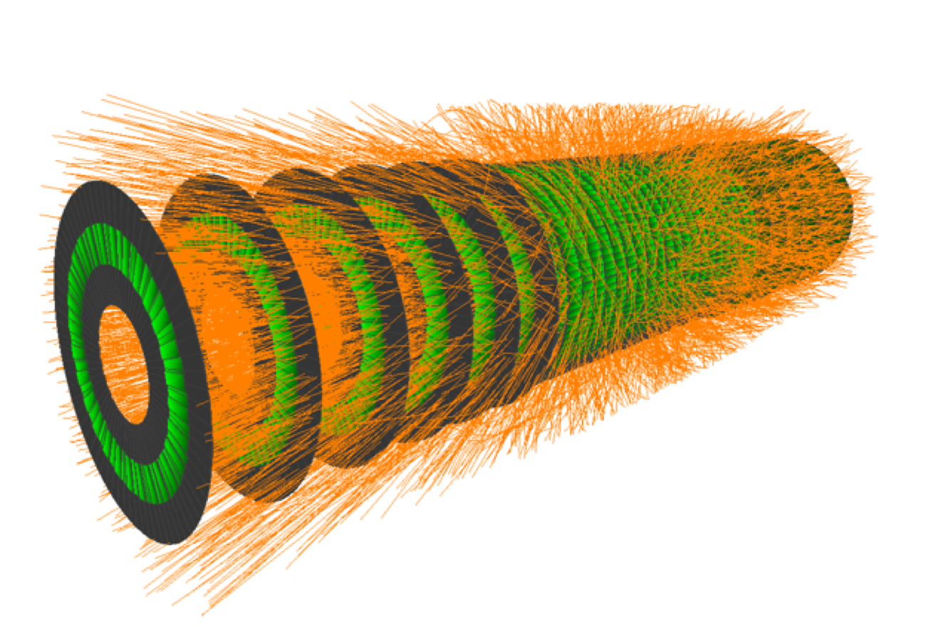![LHC](https://storage.googleapis.com/kaggle-media/competitions/CERN/cern_graphic.png)"},{"metadata":{"_cell_guid":"3cc87fff-b16d-4956-8ba2-149b187cce74","_uuid":"cf2900461153a05139d9aeb7b6502c7c91c57ea0","trusted":true},"cell_type":"code","source":"#plt.figure(figsize=(10,10))\n#plt.scatter(hits.x,hits.y, s=1)\n#plt.show()\n# Essentially the same plot as above but includes univariate plots and Pearson corr coeff\nradialview = sns.jointplot(hits.x, hits.y, size=10, s=1)\nradialview.set_axis_labels('x (mm)', 'y (mm)')\nplt.show()","execution_count":7,"outputs":[]},{"metadata":{"_cell_guid":"5b8cc4e6-cd93-4a0d-84ae-05a437d8e1f7","_uuid":"fec4a6ffadf35dacc58a9df22e28772f73cd12c9"},"cell_type":"markdown","source":"That solid core in the middle is probably more concentric detectors. Let's zoom in and find out."},{"metadata":{"_cell_guid":"46c77050-26b3-47e4-95b2-a8e8e3ae40f5","_uuid":"f9ab5775857a51aae46b9aac327b6950a9dc92b7","trusted":true},"cell_type":"code","source":"radialview = sns.jointplot( hits[hits.x.abs()<200].x, hits[hits.y.abs()<200].y, size=10, s=1)\nradialview.set_axis_labels('x (mm)', 'y (mm)')\nplt.show()","execution_count":8,"outputs":[]},{"metadata":{"_cell_guid":"ef5bad40-e37d-4ac1-843e-fadd36114bd8","_uuid":"c825f8ee638356f8830b9a0ce8ff301a4a97ce86"},"cell_type":"markdown","source":"Indeed, the inner detectors are just more concentric rings.\n\nThat scattering we see in between the rings are just events from the vertical detectors. Below shows these caps removed, and again shows the concentric nature of the inner detector."},{"metadata":{"_cell_guid":"74d94fdd-a516-4e6c-a127-64ca16c1ec42","_uuid":"a548905f0043648b70dc274de0fe52ce8e35b534","trusted":true},"cell_type":"code","source":"nocap = hits[hits.z.abs()<200]\nradialview = sns.jointplot( nocap[nocap.x.abs()<200].x, nocap[nocap.y.abs()<200].y, size=10, s=1)\nradialview.set_axis_labels('x (mm)', 'y (mm)')\nplt.show()","execution_count":9,"outputs":[]},{"metadata":{"_cell_guid":"dc0b753a-eb41-42cc-a834-c155024234d0","_uuid":"765996abc8dd103ed175319f09608c6a6fda5743"},"cell_type":"markdown","source":"Notice those clipped detectors at the corners? Notice how they seem to be layered? That's because they are small flat rectangles shingled into this pattern. Let's zoom in even more to the center-most ones."},{"metadata":{"_cell_guid":"b1573176-63f7-4f13-bc65-3a248f4df20e","_uuid":"b4074b457b9feb3c319c9848f2eeec8628a6415d","trusted":true},"cell_type":"code","source":"radialview = sns.jointplot( nocap[nocap.x.abs()<50].x, nocap[nocap.y.abs()<50].y, size=10, s=1)\nradialview.set_axis_labels('x (mm)', 'y (mm)')\nplt.show()","execution_count":10,"outputs":[]},{"metadata":{"_cell_guid":"a16fee97-472a-4705-bc8a-4a9d4df23028","_uuid":"7ca19701d5abaa732cb09faeff72e12d20e43644"},"cell_type":"markdown","source":"We can look at the sideview of the full detector, too."},{"metadata":{"_cell_guid":"c11d2b42-4465-494c-b5d8-ec40ced3c480","_uuid":"56d950512c9a212d957208de417f457b77443c70","trusted":true},"cell_type":"code","source":"# See here for why these two plots are not in subplots:\n# https://stackoverflow.com/a/35044845\n# There appears to be radial symmetry, so x ~= y for this visualization\n'''\nfig = plt.figure()\nsns.jointplot(hits.z, hits.y, s=1)\naxialview.set_axis_labels('z (mm)', 'y (mm)')\naxialview.fig.set_figwidth(24)\naxialview.fig.set_figheight(8)\n'''\nplt.figure(figsize=(24,8))\naxialview = plt.scatter(hits.z, hits.y, s=1) \nplt.xlabel('z (mm)')\nplt.ylabel('y (mm)')\nplt.show()","execution_count":11,"outputs":[]},{"metadata":{"_cell_guid":"333bd4b9-d434-48d5-b7bb-fa877113872a","_uuid":"3c6d41eedb9018cfaaeaeb11d3bd788b0acc5a7c"},"cell_type":"markdown","source":"For completeness, below is a 3D plot of a random sample effectively combining both of the above. Note though I could not get it to plot with proportional axes without adding a couple of points to force full axes."},{"metadata":{"_cell_guid":"a61ebdda-8074-4ebe-b671-21e46c870fbb","_uuid":"0312203ae2ee2c1db3f77d93172c72f8ccdecd04","trusted":true},"cell_type":"code","source":"plt.figure(figsize=(15,15))\nax = plt.axes(projection='3d')\nsample = hits.sample(30000)\nax.scatter(sample.z, sample.x, sample.y, s=5, alpha=0.5)\nax.set_xlabel('z (mm)')\nax.set_ylabel('x (mm)')\nax.set_zlabel('y (mm)')\n# These two added to widen the 3D space\nax.scatter(3000,3000,3000, s=0)\nax.scatter(-3000,-3000,-3000, s=0)\nplt.show()","execution_count":12,"outputs":[]},{"metadata":{"_cell_guid":"965ea794-777b-439e-af70-f7bb3e2fedda","_uuid":"fa24c868693c8231279e1638ecd9b955faba10de"},"cell_type":"markdown","source":"Normally one should bin these events with position resolution in mind. But it appears resolution is effectively perfect, or \" Depending on the detector type only one of the channel identifiers is valid, e.g. for the strip detectors, and the value might have different resolution.\" This is something I need to think on."},{"metadata":{"_cell_guid":"313872d7-eb0a-4780-978f-d25a48795010","_uuid":"dce572d1df88a259fa477ecb79f930e81eddb6d4"},"cell_type":"markdown","source":"## Where are the individual detector groups located?"},{"metadata":{"_cell_guid":"1282723d-6b15-4946-a053-907eed3c530e","_uuid":"0ba3ab76bde0555027400651c49fb4bbf069fe7c"},"cell_type":"markdown","source":"Let's plot each detector volume as a different color:"},{"metadata":{"_cell_guid":"80a175cb-5574-42b5-b1d4-5c19d0e2f80f","_uuid":"da022caf1b820242e17d7628d5fbdef556e3815d","trusted":true,"collapsed":true},"cell_type":"code","source":"# I am sure there's a nice pandas-specific method, but alas\nvolumes = hits.volume_id.unique()\n\n#plt.figure(figsize=(15,15))\n#for volume in volumes:\n#    v = hits[hits.volume_id == volume]\n#    #sns.jointplot(v.x, v.y, size=10, s=1)\n#    plt.scatter(v.x, v.y, s=10, label='Volume '+str(volume), alpha=0.5)\n#plt.title('Detector Volumes, Radial View')\n#plt.xlabel('x (mm)')\n#plt.ylabel('y (mm)')\n#plt.legend()\n#plt.show()","execution_count":24,"outputs":[]},{"metadata":{"_cell_guid":"85a4826c-31dc-4a8e-8f67-11af5ace553d","_uuid":"8967f84af239f63d4c2ec89f4fbc5d8690af0a93","trusted":true,"collapsed":true},"cell_type":"code","source":"#plt.figure(figsize=(24,8))\n#for volume in volumes:\n#    v = hits[hits.volume_id == volume]\n#    plt.scatter(v.z, v.y, s=10, label='Volume '+str(volume), alpha=0.5)\n#plt.title('Detector Volumes, Axial View')\n#plt.xlabel('z (mm)')\n#plt.ylabel('y (mm)')\n#plt.legend()\n#plt.show()","execution_count":23,"outputs":[]},{"metadata":{"_cell_guid":"1db4231e-d732-4e88-9472-4ee182ee5f04","_uuid":"570062cae3db995f363f452997c702cf92e73da4"},"cell_type":"markdown","source":"Let's ~~also~~ only plot these in 3D:"},{"metadata":{"_cell_guid":"63bc84c0-b242-40b7-9411-db3db91057b4","_uuid":"9842cde51b7b4e6e2784897980e6b09474a9f8cc","trusted":true},"cell_type":"code","source":"plt.figure(figsize=(20,20))\nax = plt.axes(projection='3d')\nfor volume in volumes:\n    v = sample[sample.volume_id == volume]\n    ax.scatter(v.z, v.x, v.y, s=5, label='Volume '+str(volume), alpha=0.5)\nax.set_xlabel('z (mm)')\nax.set_ylabel('x (mm)')\nax.set_zlabel('y (mm)')\nax.legend()\n# These two added to widen the 3D space\nax.scatter(3000,3000,3000, s=0)\nax.scatter(-3000,-3000,-3000, s=0)\nplt.show()","execution_count":15,"outputs":[]},{"metadata":{"_cell_guid":"0b91f609-4d18-4432-8f45-3dce5d99b4f7","_uuid":"257f78ee8ae0491d88b74f4413ddfc2f2027d8e1"},"cell_type":"markdown","source":"We can also look at the layers:"},{"metadata":{"_cell_guid":"bff1eaa2-22ed-48ff-8847-8f549ab40a6d","_uuid":"95f93f3459b4247d9a65f1c852face75ff20fc36","trusted":true,"collapsed":true},"cell_type":"code","source":"layers = hits.layer_id.unique()\n\n#plt.figure(figsize=(15,15))\n#for layer in layers:\n#    l = hits[hits.layer_id == layer]\n#    plt.scatter(l.x, l.y, s=10, label='Layer '+str(layer), alpha=0.5)\n#plt.title('Detector Layers, Radial View')\n#plt.xlabel('x (mm)')\n#plt.ylabel('y (mm)')\n#plt.legend()\n#plt.show()","execution_count":21,"outputs":[]},{"metadata":{"_cell_guid":"210217fb-253c-470f-9a44-9cb82b0998e5","_uuid":"6c406c474834feccdeda7a2791515804da52705f","trusted":true,"collapsed":true},"cell_type":"code","source":"#plt.figure(figsize=(24,8))\n#for layer in layers:\n#    l = hits[hits.layer_id == layer]\n#    plt.scatter(l.z, l.y, s=10, label='Layer '+str(layer), alpha=0.5)\n#plt.title('Detector Layers, Axial View')\n#plt.xlabel('z (mm)')\n#plt.ylabel('y (mm)')\n#plt.legend()\n#plt.show()","execution_count":22,"outputs":[]},{"metadata":{"_cell_guid":"4b4a137c-1d23-4668-a5d2-a5dd29274be2","_uuid":"983edfcf2445162f9f61e789c28b5f3db8b3ecba","trusted":true},"cell_type":"code","source":"plt.figure(figsize=(20,20))\nax = plt.axes(projection='3d')\nfor layer in layers:\n    l = sample[sample.layer_id == layer]\n    ax.scatter(l.z, l.x, l.y, s=5, label='Layer '+str(layer), alpha=0.5)\nax.set_xlabel('z (mm)')\nax.set_ylabel('x (mm)')\nax.set_zlabel('y (mm)')\nax.legend()\n# These two added to widen the 3D space\nax.scatter(3000,3000,3000, s=0)\nax.scatter(-3000,-3000,-3000, s=0)\nplt.show()","execution_count":18,"outputs":[]},{"metadata":{"_cell_guid":"d435b7f0-2b24-4df8-bfd3-1523d9eb1ba7","_uuid":"7286f579427d21341c8d95142e86f26a37444f05"},"cell_type":"markdown","source":"Beautiful graphs! I'll avoid plotting modules because there are way too many."},{"metadata":{"_cell_guid":"c1eeb2c1-18f5-4967-b105-e54da8fbe70a","_uuid":"acd708ce5ff125daf8c86cecef3158dd9d4a9c06"},"cell_type":"markdown","source":"## More Detector Group Inquiry"},{"metadata":{"_cell_guid":"c70e8068-a22b-4faa-8a26-a49a8c551396","_uuid":"0cfa38561f3b032d46070b314d3442bd753df0c3"},"cell_type":"markdown","source":"Remember: modules make up layers, and layers make up volumes, i.e., module_id is a subdirectory of layer_id, and layer_id is a subdirectory of volume_id. I've jumped the gun here, but cells are the smallest unit of resolution and thus a subdirectory of module_id. \nWe could look at the populations of all of these, too."},{"metadata":{"_cell_guid":"826847ea-3163-464f-ad7b-911535537f40","_uuid":"f6495e59caca12fa3c41521139cd8c62c5a08811","trusted":true},"cell_type":"code","source":"plt.figure(figsize=(30,10))\nplt.subplot(1,5,1)\nsns.distplot(hits.volume_id)\nplt.subplot(1,5,2)\nsns.distplot(hits.layer_id)\nplt.subplot(1,5,3)\nsns.distplot(hits.module_id)\nplt.subplot(1,5,4)\nsns.distplot(cells.ch0)\nplt.subplot(1,5,5)\nsns.distplot(cells.ch1)\nplt.show()","execution_count":26,"outputs":[]},{"metadata":{"_cell_guid":"8af7d104-e13f-417c-b26a-feaf1587b7f6","_uuid":"5b08e86e8a8ec8ee413bb1f2217b4d300e33e44b"},"cell_type":"markdown","source":"If I were to guess I's say low-id layer, modules, cells are closer to the center. Maybe we can do the obvious: plot hits by their radius."},{"metadata":{"_cell_guid":"165a8e61-6de7-4f86-af93-d14c44505120","_uuid":"fe4aeb66cd008d62a52dd176ea9d22982091c634","trusted":true},"cell_type":"code","source":"plt.figure(figsize=(30,10))\nradius2 = np.sqrt(hits.x**2 + hits.y**2)\nplt.subplot(1,3,1)\nsns.distplot(radius2, axlabel='sqrt(x^2 + y^2)')\nplt.subplot(1,3,2)\nradius3 = np.sqrt(hits.x**2 + hits.y**2 + hits.z**2)\nsns.distplot(radius3, axlabel='sqrt(x^2 + y^2 + z^2)')\nplt.subplot(1,3,3)\nsns.distplot(hits.z**2, axlabel='z')\nplt.show()","execution_count":27,"outputs":[]},{"metadata":{"_cell_guid":"efb93bef-d688-4763-8b8a-d337b167b7ca","_uuid":"a1a3e854bf0173cd00340f63b4096f8c7050dda1"},"cell_type":"markdown","source":"And now that we see the general distribution of events are indeed proportional to radius, let's at least plot groups by radius."},{"metadata":{"_cell_guid":"a46ebc12-de17-4325-8c82-367cc0d8cbda","_uuid":"737a6a0b0c1d6a9575eab7dbde4f2034db82ec63","trusted":true},"cell_type":"code","source":"plt.figure(figsize=(30,10))\nplt.subplot(1,3,1)\nplt.scatter(hits.volume_id, radius2)\nplt.xlabel('volume_id')\nplt.ylabel('radius')\nplt.subplot(1,3,2)\nplt.scatter(hits.layer_id, radius2)\nplt.xlabel('layer_id')\nplt.ylabel('radius')\nplt.subplot(1,3,3)\nplt.scatter(hits.module_id, radius2)\nplt.xlabel('module_id')\nplt.ylabel('radius')\nplt.show()","execution_count":28,"outputs":[]},{"metadata":{"_cell_guid":"6ef236b8-b84a-496a-b03d-7b613d334d62","_uuid":"b376bacac59df3691db045b0e697da3f8cf9af55"},"cell_type":"markdown","source":"From these:\n* Volumes are named for left, center, right of detector center\n* Layers are named for their radius from the detector center, like onion layers\n* Modules are named for their rotation about the detector center\n\nWe can see this visually in the 3D plots above, too."},{"metadata":{"_cell_guid":"29a6153a-1ebf-4c8c-ac8d-dd5bc3865343","_uuid":"0b12245b1cb2431b388f0cf6b9bda094c5cac75e"},"cell_type":"markdown","source":"Just checking out group distrubution here:"},{"metadata":{"_cell_guid":"9a3e52f1-c1e6-4342-8464-f33e0ae2cac5","_uuid":"4a967af65928467ecbbb03bb60ee11965763c308","trusted":true},"cell_type":"code","source":"hits.volume_id.value_counts()","execution_count":29,"outputs":[]},{"metadata":{"_cell_guid":"e5de8687-32e8-4fe7-9133-34ddaed07091","_uuid":"3049f286d66d6cdcacdb0ace3a70eec3e2db831a","trusted":true},"cell_type":"code","source":"hits.layer_id.value_counts()","execution_count":30,"outputs":[]},{"metadata":{"_cell_guid":"53463f90-3548-48a1-aa4e-a4e49f19a6ba","_uuid":"ea353896a5bb819dc47da31c48b7530da74690ea","trusted":true},"cell_type":"code","source":"hits.module_id.value_counts().head()","execution_count":31,"outputs":[]},{"metadata":{"_cell_guid":"089285eb-547b-4026-adc5-a595e5ab7a6e","_uuid":"f5e8a221e7d08fb8680b9dd1519570b3aa6f5dbb","collapsed":true,"trusted":true},"cell_type":"code","source":"#groups = hits.groupby(['volume_id', 'layer_id', 'module_id'])","execution_count":32,"outputs":[]},{"metadata":{"_cell_guid":"a6659243-e5ca-4166-8459-c6261caa499a","_uuid":"e3a9285986a2f40530337fb707d1e455fdd10236"},"cell_type":"markdown","source":"## Hit Feature Correlations\n\nPlotting each feature (x, y, z, volume, layer, module) against each other. ~~I've dropped hits_id because that is a scientist-given variable and not physics-relevant.~~"},{"metadata":{"_cell_guid":"44b6e381-9f15-403a-b3aa-c2c44bb3a9a5","_uuid":"bd3ce57e3591df29054af2a8fc7633b9f50bb8cf","trusted":true},"cell_type":"code","source":"# Pairplotting 120k hits takes too long, so let's look at a random sampling\n#sample = hits.drop('hit_id', axis=1).sample(3000)\nsample = hits.sample(3000)\n# I've also decided to color-code them by group again. Makes sense to me.\nsns.pairplot(sample, hue='volume_id', size=8)\nplt.show()","execution_count":33,"outputs":[]},{"metadata":{"_cell_guid":"4b0689ab-f021-4d05-8126-14a2264a0a42","_uuid":"a7f2963e6d30c682548699b0f53d2166e6010949"},"cell_type":"markdown","source":"Qualitatively, there definitely exists correlations between hit features. We can extract the useable ones fairly easily (I think -- I may have done something like this a while ago) but I'll move on for now.\n\nWe can also plot a correlation heatmap. Now _here_ I've dropped hits_id."},{"metadata":{"_cell_guid":"28f1c012-f450-48dd-8744-9a0d72a5bed2","_uuid":"15cae8c04eee215d53b724b6197b15728eaee57a","trusted":true},"cell_type":"code","source":"plt.figure(figsize=(10, 10))\nhitscorr = hits.drop('hit_id', axis=1).corr()\nsns.heatmap(hitscorr, cmap='coolwarm', square=True)\nplt.title('Hits Correlation Heatmap')\nplt.show()","execution_count":34,"outputs":[]},{"metadata":{"_cell_guid":"64fbd7a1-d531-4506-b1bb-e4108356094c","_uuid":"447e7961ab6a7ee79854296823c9b3f522e262a8"},"cell_type":"markdown","source":"I suppose it does make sense that module_id is correlated with layer_id, and layer_id is correlated with volume_id."},{"metadata":{"_cell_guid":"9502cdee-fe11-4dd2-aeb8-9bbe3c019dd2","_uuid":"57ece65573ca23eabf5c01602a07b92b2dd36f12"},"cell_type":"markdown","source":"# <a name=\"cells\">Cells</a>\nThe cells file contains the constituent active detector cells that comprise each hit. The cells can be used to refine the hit to track association. A cell is the smallest granularity inside each detector module, much like a pixel on a screen, except that depending on the volume_id a cell can be a square or a long rectangle. It is identified by two channel identifiers that are unique within each detector module and encode the position, much like column/row numbers of a matrix. A cell can provide signal information that the detector module has recorded in addition to the position. Depending on the detector type only one of the channel identifiers is valid, e.g. for the strip detectors, and the value might have different resolution.  \n* __hit_id__: numerical identifier of the hit as defined in the hits file.\n* __ch0, ch1__: channel identifier/coordinates unique within one module.\n* __value__: signal value information, e.g. how much charge a particle has deposited."},{"metadata":{"_cell_guid":"4e8ddd37-39d3-4da7-ab1f-a51d51a792aa","_uuid":"211081d228593c5db775d0ec4ff2c7a9e6cf1b22","trusted":true},"cell_type":"code","source":"cells.head()","execution_count":35,"outputs":[]},{"metadata":{"_cell_guid":"b3367ab0-ecd0-443a-8cb3-4da7fca0c659","_uuid":"fb70307153bd6c5ec829a63a8e55610409347c78","trusted":true},"cell_type":"code","source":"cells.tail()","execution_count":36,"outputs":[]},{"metadata":{"_cell_guid":"8b47c942-e753-4410-9d32-bc0b64736a29","_uuid":"8180e3b71268f3fdc2560593ebed56e2be578c83","trusted":true},"cell_type":"code","source":"cells.describe()","execution_count":37,"outputs":[]},{"metadata":{"_cell_guid":"87ff2aa6-2868-4bff-83af-258f335d4752","_uuid":"59fb8c099f230860fb3f6ccf9239182fe80ae212","trusted":true},"cell_type":"code","source":"plt.figure(figsize=(10, 10))\ncellscorr = cells.drop('hit_id', axis=1).corr()\nsns.heatmap(cellscorr, cmap='coolwarm', square=True)\nplt.title('Cells Correlation Heatmap')\nplt.show()","execution_count":38,"outputs":[]},{"metadata":{"_cell_guid":"aae05ff9-3589-4e60-80b3-f51f395b1b2f","_uuid":"28980ff04d88be785d2d1abf37a24549f34376e2"},"cell_type":"markdown","source":"# <a name=\"particles\">Particles</a>\nThe particles files contains the following values for each particle/entry:  \n* __particle_id__: numerical identifier of the particle inside the event.\n* __vx, vy, vz__: initial position or vertex (in millimeters) in global coordinates.\n* __px, py, pz__: initial momentum (in GeV/c) along each global axis.\n* __q__: particle charge (as multiple of the absolute electron charge).\n* __nhits__: number of hits generated by this particle."},{"metadata":{"_cell_guid":"f8ea9079-2125-43cc-8d54-e236ce7ec095","_uuid":"3883c1f3f89aff89eacedd3c6b71155bf1719eee","trusted":true},"cell_type":"code","source":"particles.head()","execution_count":39,"outputs":[]},{"metadata":{"_cell_guid":"8c95bd30-4211-4cce-904b-c3371e847bfc","_uuid":"d7336ed4b40639404335d06e9906499713a5f9d3","trusted":true},"cell_type":"code","source":"particles.tail()","execution_count":40,"outputs":[]},{"metadata":{"_cell_guid":"151ae475-7f48-466e-a394-21d3297cb7bb","_uuid":"63f5e3e3279ed92541069c5bc03524e96b8380c2","trusted":true},"cell_type":"code","source":"particles.describe()","execution_count":41,"outputs":[]},{"metadata":{"_cell_guid":"c667a523-631f-424c-baff-e220902b9e2c","_uuid":"427cd88dd28a916cf10cd15e71e4e8bbcfc7462f"},"cell_type":"markdown","source":"Some things to noe here:\n* The particle vertex does not necessarily have to be the center of the detector. Perhaps that means it is a secondary particle created later inside the detector, either from a collison or a decay.\n* Charge _q_ is always +1 or -1, not some larger integer. No ions here.\n* nhits can be as low as 0. How? Not sure yet.\n\nEdit: Thanks to Nadans, nhits can be 0 when they hit no cell (obvously). What was not obvious was why particles that hit nothing would be kept in this simulation. After all, a particle that does not interact is not observed -- though could be inferenced. Anyway, Nadans noted that a particle moving along the beamline has a nonzero chance of not interacting at al, missing all the detectorsl. Let's see if we can prove this."},{"metadata":{"trusted":true,"_uuid":"88c463c7af89fca6b95133707f70ed6a37cda246"},"cell_type":"code","source":"nhits0 = particles[particles.nhits ==0]\nnhits0_2 = nhits0[nhits0.particle_id == 4503805785800704]\nnhits0[['px','py','pz']].describe()","execution_count":52,"outputs":[]},{"metadata":{"trusted":true,"_uuid":"1a9f8e407168137f5bd5aa756cc493efb07a345f"},"cell_type":"code","source":"pt_mean = np.mean(np.sqrt(particles.px**2 + particles.py**2))\npt_mean_unc = np.std(np.sqrt(particles.px**2 + particles.py**2))\npt0_mean = np.mean(np.sqrt(nhits0.px**2 + nhits0.py**2))\npt0_mean_unc = np.std(np.sqrt(nhits0.px**2 + nhits0.py**2))\nprint('Mean transverse momentum:')\nprint('    full:', pt_mean, ' +-', pt_mean_unc, 'GeV/c')\nprint(' nhits=0:', pt0_mean, '+-', pt0_mean_unc)","execution_count":74,"outputs":[]},{"metadata":{"_uuid":"1566ec153297b6dc436d5bd072f18e053dc2cfff"},"cell_type":"markdown","source":"From the describe(), the mean z-momentum is actually 10x _less for particles with nhits=0 than the full particles dataset. Compare 0.017 +- 4.2 GeV/c here to 0.1 +- 7.8 Gev/c.  \nFrom the printout, the mean t-momentum is again smaller, though not as much.  \nPerhaps particles with less total monetum just interact less.\nAre these points significant enough to conclude Nadans hypotheses? Not really. We'll leave this for now."},{"metadata":{"_cell_guid":"e8385029-819c-4f70-a0c2-07f751c8935f","_uuid":"94d49b138efe0bc1b2d167e4d15700d5473feab5"},"cell_type":"markdown","source":"Let's plot a couple of histograms:"},{"metadata":{"_cell_guid":"3a79bfee-6620-4751-ac4f-0381655c330b","_uuid":"4dc97c275d86e9c93a9c3c4a78dc4f3f03977777","trusted":true},"cell_type":"code","source":"plt.figure(figsize=(15,10))\nplt.subplot(1,2,1)\nparticles.q.hist(bins=3)\nplt.xlabel('Charge (e)')\nplt.ylabel('Counts')\nplt.subplot(1,2,2)\nparticles.nhits.hist(bins=particles.nhits.max())\nplt.xlabel('nhits')\nplt.show()","execution_count":75,"outputs":[]},{"metadata":{"_cell_guid":"843958d6-c9d9-4aa6-a413-e63df9eb8d7a","_uuid":"2c600cba989662caf0b0fb4908bf9ece131c857d"},"cell_type":"markdown","source":"There appears to be about a 20% differenence betweeen positively and negatively charged particles, i.e. there are more positively charged particles. And for nhits, the majority are either 0 or centered around some gaussian at 12. We should eventualy be able to convolve nhits and momentum."},{"metadata":{"_cell_guid":"3d824c8a-e118-4682-84d1-8128e924d888","_uuid":"81c001f0866aecb4b6cb3e64cc6d59762c0b8654"},"cell_type":"markdown","source":"Back to nhits and momentum... I'd say that nhits is proportional to total momentum p (particle has enough energy (but not too much) to move through enough detectors before stopping). Is this true? Or, assuming a particle does not stop or decay, then it would be dependent on where inside the detector this particle was and where it was going."},{"metadata":{"_cell_guid":"73aa7b42-4368-4908-9844-7d0ea6b4b402","_uuid":"44dbced5fc91f151cd641b0ebd5a76dde7256f1b","trusted":true},"cell_type":"code","source":"plt.figure(figsize=(10,10))\np = np.sqrt(particles.px**2 + particles.py**2 + particles.pz**2)\nplt.scatter(particles.nhits, p)\nplt.yscale('log')\nplt.xlabel('nhits')\nplt.ylabel('Momentum (GeV/c)')\nplt.show()","execution_count":76,"outputs":[]},{"metadata":{"_cell_guid":"939f460e-41f4-4756-95a6-b0401af5523e","_uuid":"deb2ec427f51c345ed9f7f4e642b266e28e6b8d9"},"cell_type":"markdown","source":"Wow, I see no real correlation here... For now.\n\nWe can look at a histogram of momentum (note the log~~-log~~ axes):"},{"metadata":{"_cell_guid":"13d968cf-46f0-41b8-ad28-b1b25d68de61","_uuid":"0dabc21bab3215bb33e307b4082fde4121a7f724","trusted":true},"cell_type":"code","source":"plt.figure(figsize=(15,8))\nplt.subplot(1,2,1)\n#plt.xscale('log')\nplt.hist(np.sqrt(particles.px**2 + particles.py**2), bins=100, log=True)\nplt.xlabel('Transverse momentum (GeV/c)')\nplt.ylabel('Counts')\nplt.subplot(1,2,2)\n#plt.xscale('log')\nplt.hist(particles.pz.abs(), bins=100, log=True)\nplt.xlabel('Z momentum (GeV/C)')\nplt.show()","execution_count":77,"outputs":[]},{"metadata":{"_cell_guid":"ac478dab-7cb4-4980-8364-040165b20793","_uuid":"8bf69406463173311dd8a2f0e9271a0a91311b32"},"cell_type":"markdown","source":"Right now I'm not sure what this tells us about momentum other than most particles have \"low\" momentum and few have \"high\" momentum. What about these momentums wrt eachother?"},{"metadata":{"_cell_guid":"71efd893-b1b4-4314-9ae1-444395932fa8","_uuid":"ebfa232d7db4b9292d64aea513e25db89b97e647","trusted":true},"cell_type":"code","source":"plt.figure(figsize=(10,10))\nplt.scatter(np.sqrt(particles.px**2 + particles.py**2), particles.pz, s=1)\nplt.xscale('log')\n#plt.yscale('log')\nplt.xlabel('Transverse momentum (GeV/c)')\nplt.ylabel('Z momentum (GeV/C)')\n#plt.zlabel('Counts')\nplt.show()","execution_count":78,"outputs":[]},{"metadata":{"_cell_guid":"c2473a01-a935-47ac-8485-e08fe870f520","_uuid":"c826d6b7586376e009388726e376532ff613824b"},"cell_type":"markdown","source":"Man, that one _pz_=500 particle is messing with our plot. Clip it and other outliers:"},{"metadata":{"_cell_guid":"fd13b9fb-a98f-4f50-8b08-97d8c778a5fe","_uuid":"23fb727a27cc3027324424d4205a1cf918de4de0","trusted":true},"cell_type":"code","source":"p = particles[particles.pz < 200]\n\nplt.figure(figsize=(10,10))\nplt.scatter(np.sqrt(p.px**2 + p.py**2), p.pz, s=5, alpha=0.5)\nplt.plot([0.1,0.1],[p.pz.min(),p.pz.max()], c='g') # 0.1 instead of 0 because log plot.\nplt.plot([0.1,np.sqrt(p.px**2 + p.py**2).max()],[0.1,0.1], c='r', linestyle='--')\nplt.xscale('log')\n#plt.yscale('log')\nplt.xlabel('Transverse momentum (GeV/c)')\nplt.ylabel('Z momentum (GeV/C)')\nplt.show()","execution_count":82,"outputs":[]},{"metadata":{"_cell_guid":"9b6eda5e-bd39-4694-b12b-0699949a1958","_uuid":"086a6bc86c7ee97ff455f3bfe8d7ab6c74a51656"},"cell_type":"markdown","source":"Particles that lie about the green line were moving in a trajectory perfectly parallel to the beamline. Particles that lie about the red dashed line were moving in a trajectory perfectly transverse to the beamline. From this we can see that move particles were travelling in some sort of cone shape, psuedocoincidentally shown as a cone here. Here I am using the fact that momentum is of course a magnitude and a direction."},{"metadata":{"_uuid":"85744e2637bc96b5b225f96c5539ef4ebb195eba"},"cell_type":"markdown","source":"I'm also curious about where these particles start (vertex) and what their momentum is. Is there correlation?"},{"metadata":{"trusted":true,"_uuid":"d69d21804f9ae24500d2d6b004096178cda91a82"},"cell_type":"code","source":"plt.figure(figsize=(20,10))\nplt.subplot(1,2,1)\nplt.scatter(particles.vx, particles.vy, s=1)\nplt.xlabel('px')\nplt.ylabel('py')\nplt.subplot(1,2,2)\nplt.scatter(particles.vz, particles.vy, s=1)\nplt.xlabel('pz')\nplt.show()","execution_count":115,"outputs":[]},{"metadata":{"trusted":true,"_uuid":"9266aa60b7f56cd5fb653b4bf0befd74bbd1da34"},"cell_type":"code","source":"plt.figure(figsize=(20,10))\nplt.subplot(1,2,1)\nplt.scatter(np.sqrt(particles.vx**2+particles.vy**2), np.sqrt(particles.px**2+particles.py**2), s=1)\nplt.xlabel('Vertex radius, 2D (mm)')\nplt.ylabel('Transverse momentum (GeV/c)')\nplt.xscale('log')\nplt.yscale('log')\nplt.subplot(1,2,2)\nplt.scatter(np.sqrt(particles.vx**2+particles.vy**2+particles.vz**2), np.sqrt(particles.px**2+particles.py**2+particles.pz**2), s=1)\nplt.xlabel('Vertex radius, 3D (mm)')\nplt.ylabel('Total momentum (GeV/c)')\nplt.xscale('log')\nplt.yscale('log')\nplt.show()","execution_count":103,"outputs":[]},{"metadata":{"_uuid":"a123659681aae2de6686f6548299a7415f785e1b"},"cell_type":"markdown","source":"It seems particles of ~all momentums exist at all points. Interesting, though, that particle vertices seem to coincide with detector strips, i.e. they are _created_ not only at the beam but after interacting with the detectors. See below, each particle vertex is unique and not just 1 of 10 hits, e.g.."},{"metadata":{"trusted":true,"_uuid":"e0d630d46b12334ac319b524ec4c98c870d2d412"},"cell_type":"code","source":"len(particles), len(particles.particle_id.unique())","execution_count":99,"outputs":[]},{"metadata":{"_cell_guid":"b761824b-42ba-4fe8-aba3-9d4a325a0653","_uuid":"40265d6cd72491ec6b1b1fc29e450df841446b8d","trusted":true},"cell_type":"code","source":"plt.figure(figsize=(10, 10))\nparticlescorr = particles.drop('particle_id', axis=1).corr()\nsns.heatmap(particlescorr, cmap='coolwarm', square=True)\nplt.title('Particles Correlation Heatmap')\nplt.show()","execution_count":83,"outputs":[]},{"metadata":{"_cell_guid":"d945c36b-e943-433e-89cf-9846d98bb422","_uuid":"2259aa9cac68243611d95bba2469a1da9f86e350"},"cell_type":"markdown","source":"# <a name=\"truth\">Truth</a>\nThe truth file contains the mapping between hits and generating particles and the true particle state at each measured hit. Each entry maps one hit to one particle.  \n* __hit_id__: numerical identifier of the hit as defined in the hits file.\n* __particle_id__: numerical identifier of the generating particle as defined in the particles file. A value of 0 means that the hit did not originate from a reconstructible particle, but e.g. from detector noise.\n* __tx, ty, tz__ true intersection point in global coordinates (in millimeters) between the particle trajectory and the sensitive surface.\n* __tpx, tpy, tpz__ true particle momentum (in GeV/c) in the global coordinate system at the intersection point. The corresponding vector is tangent to the particle trajectory at the intersection point.\n* __weight__ per-hit weight used for the scoring metric; total sum of weights within one event equals to one."},{"metadata":{"_cell_guid":"6b507837-5c9b-4626-aef8-dfce7785b3e3","_uuid":"34c1a9e8e6a54c785cce1048b3a382d012aee871","trusted":true},"cell_type":"code","source":"truth.head()","execution_count":84,"outputs":[]},{"metadata":{"_cell_guid":"d9e52edf-460f-42af-8438-f49de85b5fdc","_uuid":"df4b93821ae5f4c3fe6e10212b96edab4275ea39","trusted":true},"cell_type":"code","source":"truth.tail()","execution_count":85,"outputs":[]},{"metadata":{"_cell_guid":"72dd1cc3-ccb6-414a-9e4e-fcb4ce065495","_uuid":"9e33bf88a1a33a1eda9b5298da74914f3c2f0631","collapsed":true,"trusted":true},"cell_type":"code","source":"# Just checking out one example\n#truth[truth.particle_id == 22525763437723648]","execution_count":86,"outputs":[]},{"metadata":{"_cell_guid":"29e79fb7-945c-43c8-abc1-566b3df59e1a","_uuid":"0516a4c2be878cb5d2ce03058ea01d2c3bbfefe2","trusted":true},"cell_type":"code","source":"# Number of unique particles\nlen(truth.particle_id.unique())","execution_count":87,"outputs":[]},{"metadata":{"_cell_guid":"46ed030e-eda3-4ee5-b4d7-b062a3362ec3","_uuid":"7deffb227ecbce2e9a17d0d39c0dab6272f88976"},"cell_type":"markdown","source":"## Let's plot some particle tracks"},{"metadata":{"_cell_guid":"b27d8917-3f0a-4dd6-85e6-c15a2940b807","_uuid":"26c0c25dc8183694f40da00b05e4914edf7a853e","trusted":true},"cell_type":"code","source":"# Get every 100th particle\ntracks = truth.particle_id.unique()[1::100]\n\nplt.figure(figsize=(15,15))\nax = plt.axes(projection='3d')\nfor track in tracks:\n    t = truth[truth.particle_id == track]\n    ax.plot3D(t.tz, t.tx, t.ty)\nax.set_xlabel('z (mm)')\nax.set_ylabel('x (mm)')\nax.set_zlabel('y (mm)')\n# These two added to widen the 3D space\nax.scatter(3000,3000,3000, s=0)\nax.scatter(-3000,-3000,-3000, s=0)\nplt.show()","execution_count":88,"outputs":[]},{"metadata":{"_cell_guid":"a9d4441f-3d3a-4bac-ab3e-834af2dd4d60","_uuid":"3199a8428755e908fbff89a4a88aca31a8472c60","collapsed":true},"cell_type":"markdown","source":"We can actually see that indeed many particles do not start at the detector center, and originate somewhere else. We can also see that trajectories are more (visibly) helical the less z-momentum they have."},{"metadata":{"collapsed":true,"trusted":true,"_uuid":"496a9f19d752e9ab020f017f8e3d974288cd939f"},"cell_type":"code","source":"","execution_count":null,"outputs":[]}],"metadata":{"kernelspec":{"display_name":"Python 3","language":"python","name":"python3"},"language_info":{"name":"python","version":"3.6.5","mimetype":"text/x-python","codemirror_mode":{"name":"ipython","version":3},"pygments_lexer":"ipython3","nbconvert_exporter":"python","file_extension":".py"}},"nbformat":4,"nbformat_minor":1}