{"cells":[{"metadata":{"_cell_guid":"99c702eb-f95c-4403-ac4f-69aeaa653e8e","_uuid":"a458131750431a9f761e87eb36e94489609d8884"},"cell_type":"markdown","source":"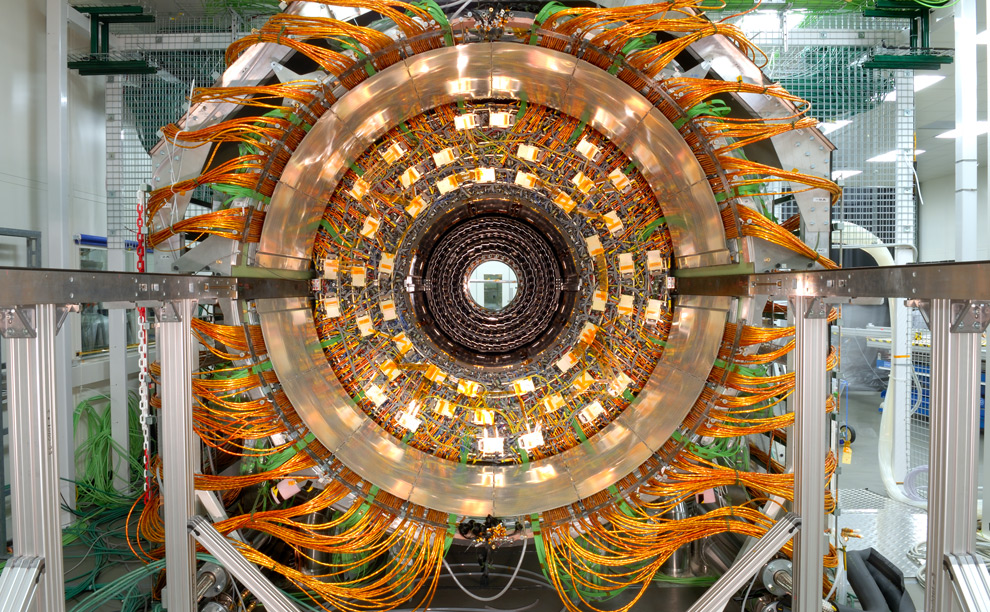"},{"metadata":{"_cell_guid":"b89b8bc7-587b-46cf-9e3b-022bd5a8ae3d","_uuid":"05a51ccbcf4c2c663fdca26ec8b81f635f94de56"},"cell_type":"markdown","source":"# Please wait few seconds to display graphs/images because plotly is little slow.\n## More To Come !! Stayed Tuned."},{"metadata":{"_cell_guid":"d0bc4f72-629d-4f20-8cb2-e4555a97ee93","_uuid":"006839cecc1945c1ec066ed602ef4739ccc339fc"},"cell_type":"markdown","source":"- 1. Introduction\n- 2. Importing required libraries and data\n- 3. Event hits Data\n - 3.1 Glimpse of Event hit data\n - 3.2 Vertical Intersection ( x,y ) in Detection Layers\n - 3.3 2D scatter plot \n - 3.4 2D Histogram\n - 3.5 3D Surface plot\n - 3.6 3D Sactter plot\n - 3.7 Horizontal Intersection ( z ,y ) in Detection Layers\n - 3.8 Distribution of Volume id, Layer id and Module id for single event<\n - 3.9 ScatterPlotMatrix of full hits table\n- 4. Event hit cells data\n - 4.1 Glimpse of Event hit cells data\n - 4.2 Visualization of channel identifier/coordinates unique within one module.\n - 4.3 Channel identifiers (ch0, ch1) and signal value information for a single event\n - 4.4 ScatterPlotMatrix of Event hits cells \n- 5. Event particles Data \n - 5.1 Glimpse of Event particles data\n - 5.2 Initial position or vertex (in millimeters) in global coordinates. 'X' and 'Y' axis with number of hits generated by particular particle\n - 5.3 Distribution of particle charges in event000001005\n - 5.4 initial position or vertex (in millimeters) in global coordinates. 'X' and 'Y' axis with particle charge(positive or negative)\n - 5.5 Initial momentum (in GeV/c) along 'X' and 'Y' axis with particle charges(Positive or Negative).\n - 5.6 3D scatter plot of inintial momentum and initial vertex\n - 5.7 Initial position or vertex (in millimeters) in global coordinates. 'Z' and 'Y' axis with number of hits generated by particular particle\n - 5.8 initial momentum (in GeV/c) along 'X' and 'Y' global axis with number of hits and physics particles\n - 5.9 Distribution of number of hits generated by particular particle\n- 6. Event truth data\n - 6.1 Glimpse of Event truth data\n - 6.2 Vertical Intersection ( x,y ) between the particle trajectory and the sensitive surface\n - 6.3 Horizontal Intersection ( z,y ) between the particle trajectory and the sensitive surface\n - 6.4 3D scatter plot of true particle momentum (in GeV/c) in the global coordinate system at the intersection point\n - 6.5 Distribution of Hit ID, Particle ID and weight for each measurement hit\n- 7. Detector Geometry Information data\n - 7.1 Glimpse of Detector Geometry Information data\n - 7.2 Distribution of module_t (thickness of the detector module (in millimeter)).\n - 7.3 Distribution of module_hv ( the half-length of the module boundary along the local v direction (in millimeter)).\n - 7.4 Correlation of features\n - 7.5 Distribution of Layer ID, Volume ID and Module ID of detector Geometry information data\n - 7.6 Distribution of the size of detector cells along the local u and v direction (in millimeter)"},{"metadata":{"_cell_guid":"aa2b1cc4-630f-44ed-839e-5b87bce612d9","_uuid":"5fef0ac2337cc2b3fbc357e48f0b3618c25ca391"},"cell_type":"markdown","source":"# 1. Introduction"},{"metadata":{"_cell_guid":"877f0139-e86d-41bf-bdcc-8b6f0c1d93c8","_uuid":"50353b6a56422747a06ff324a7b5e4560e1b182a"},"cell_type":"markdown","source":"To explore what our universe is made of, scientists at CERN are colliding protons, essentially recreating mini big bangs, and meticulously observing these collisions with intricate silicon detectors.\n\nWhile orchestrating the collisions and observations is already a massive scientific accomplishment, analyzing the enormous amounts of data produced from the experiments is becoming an overwhelming challenge.\n\nEvent rates have already reached hundreds of millions of collisions per second, meaning physicists must sift through tens of petabytes of data per year. And, as the resolution of detectors improve, ever better software is needed for real-time pre-processing and filtering of the most promising events, producing even more data.\n\nTo help address this problem, a team of Machine Learning experts and physics scientists working at CERN (the world largest high energy physics laboratory), has partnered with Kaggle and prestigious sponsors to answer the question: can machine learning assist high energy physics in discovering and characterizing new particles?\n\nSpecifically, in this competition, you’re challenged to build an algorithm that quickly reconstructs particle tracks from 3D points left in the silicon detectors. "},{"metadata":{"_cell_guid":"b37f3b08-34d3-4dce-a88d-c931d185d0aa","_uuid":"ba689f496a67545995c058f05cd34b2ee7a2ae71"},"cell_type":"markdown","source":"# 2. Importing required libraries and data"},{"metadata":{"_cell_guid":"b1076dfc-b9ad-4769-8c92-a6c4dae69d19","_kg_hide-input":true,"_uuid":"8f2839f25d086af736a60e9eeb907d3b93b6e0e5","collapsed":true,"trusted":true},"cell_type":"code","source":"import numpy as np\nimport pandas as pd\nimport matplotlib.pyplot as plt\n\n# import seaborn\nimport seaborn as sns\n\n# import plotly and offline mode\nfrom plotly.offline import iplot, init_notebook_mode\nimport plotly.graph_objs as go\nimport plotly.figure_factory as ff\n\n# import cufflinks and offline mode\nimport cufflinks as cf\ncf.go_offline()\n\n% matplotlib inline\n\n# # for 3D plotting\n# import ipyvolume as ipv\n# import ipywidgets as widgets\n\nfrom trackml.dataset import load_event, load_dataset\nfrom trackml.randomize import shuffle_hits\nfrom trackml.score import score_event","execution_count":null,"outputs":[]},{"metadata":{"_cell_guid":"79c7e3d0-c299-4dcb-8224-4455121ee9b0","_kg_hide-input":true,"_uuid":"d629ff2d2480ee46fbb7e2d37f6b5fab8052498a","collapsed":true,"trusted":true},"cell_type":"code","source":"hits, cells, particles, truth = load_event('../input/train_1/event000001005')\ndetectors = pd.read_csv(\"../input/detectors.csv\")","execution_count":null,"outputs":[]},{"metadata":{"_cell_guid":"2b7f8871-ba62-4161-8dbd-59ae5f7cf0a9","_uuid":"a2b6ccf2e8efe9c0ed9f956684bd523eb3954f7e"},"cell_type":"markdown","source":"# 3. Event hits Data"},{"metadata":{"_cell_guid":"c8c3bd86-26a1-4ce2-b33f-0fd37d00b778","_uuid":"b95068a0152534082a766f9a20f34353122dfaf8"},"cell_type":"markdown","source":"## 3.1 Glimpse of Event hit data"},{"metadata":{"_cell_guid":"745cc9ad-cfb7-42ba-9823-1f4bcc93090c","_kg_hide-input":true,"_uuid":"f21ce7976fb8b8092e31c61fd78aaaa6c222783d","collapsed":true,"scrolled":true,"trusted":true},"cell_type":"code","source":"hits.head()","execution_count":null,"outputs":[]},{"metadata":{"_cell_guid":"33c66981-00d9-4d97-a4da-776792f45939","_uuid":"3cfc3dcac2718d7fdeff84add6bcd67412ca2d01"},"cell_type":"markdown","source":"The hits file contains the following values for each hit/entry:\n\n- **hit_id:** numerical identifier of the hit inside the event.\n- **x, y, z:** measured x, y, z position (in millimeter) of the hit in global coordinates.\n- **volume_id:** numerical identifier of the detector group.\n- **layer_id:** numerical identifier of the detector layer inside the group.\n- **module_id:** numerical identifier of the detector module inside the layer.\n\nThe volume/layer/module id could in principle be deduced from x, y, z. They are given here to simplify detector-specific data handling."},{"metadata":{"_cell_guid":"be3d1434-7220-4846-8fd7-ff1a669e858b","_uuid":"4476d014b7291263017056e3a16e4d54c4309196"},"cell_type":"markdown","source":"## 3.2 Vertical Intersection ( x,y ) in Detection Layers"},{"metadata":{"_cell_guid":"1375a151-93aa-4a43-b17a-106097ed820a","_kg_hide-input":true,"_uuid":"82e41eab45131c8fa42d94961cdefe2a646af2ef","collapsed":true,"trusted":true},"cell_type":"code","source":"hits_samples = hits.sample(8000)\n\nfig = ff.create_facet_grid(\n hits_samples,\n x='x',\n y='y',\n color_name='volume_id',\n show_boxes=False,\n marker={'size': 10, 'opacity': 1.0},\n )\niplot(fig, filename='facet - custom colormap')","execution_count":null,"outputs":[]},{"metadata":{"_cell_guid":"473884ba-2621-4523-83fc-238c96e5d66d","_kg_hide-input":true,"_uuid":"ab21d0e2c4b7eeecac479619d4a8575d7e054601","collapsed":true,"trusted":true},"cell_type":"code","source":"hits_samples = hits.sample(8000)\n\nfig = ff.create_facet_grid(\n hits_samples,\n x='x',\n y='y',\n facet_col='volume_id',\n color_name='volume_id',\n color_is_cat=True,\n# color_name='volume_id',\n# show_boxes=False,\n# marker={'size': 10, 'opacity': 1.0},\n )\niplot(fig, filename='facet - custom colormap')","execution_count":null,"outputs":[]},{"metadata":{"_cell_guid":"7586aeb8-b2c5-4a1b-a6c3-a7fbabc0a2c7","_uuid":"3549246c650cb51426eb7e4aafbc3a24f4239998"},"cell_type":"markdown","source":"## 3.3 2D scatter plot "},{"metadata":{"_cell_guid":"a6c19759-97cf-4a43-8e4f-48958f1b2777","_kg_hide-input":true,"_uuid":"4d7aaa0d311dba3412a2ff287b054f9ae5d439eb","collapsed":true,"scrolled":true,"trusted":true},"cell_type":"code","source":"hits_samples = hits.sample(8000)\nhits_samples.iplot(kind='scatter',x='x',y='y',mode='markers',size=10)","execution_count":null,"outputs":[]},{"metadata":{"_cell_guid":"35fa42b3-a7e7-4242-b99e-56b3233f4bf3","_uuid":"bcb632fe350fa5fe4da4e5584b94675cd96d010a"},"cell_type":"markdown","source":"## 3.4 2D Histogram"},{"metadata":{"_cell_guid":"5045053a-55f0-49f0-990a-a7204721b286","_kg_hide-input":true,"_uuid":"fb16d2657b21da2199458c3df6ee2d93604f2745","collapsed":true,"trusted":true},"cell_type":"code","source":"data = [\n go.Histogram2d(\n x=hits.x,\n y=hits.y\n )\n]\niplot(data)","execution_count":null,"outputs":[]},{"metadata":{"_cell_guid":"4071075f-7ba4-4b17-b926-8b19b4705fae","_uuid":"8cb1ae732a16b07f79bdb30d2e4439109a80896f"},"cell_type":"markdown","source":"## 3.5 3D Surface plot"},{"metadata":{"_cell_guid":"9be62bfd-4367-4f0e-bea5-6d8867f97153","_kg_hide-input":true,"_uuid":"be97d91751fa8ac240b77a5ccf2de3adb14698ee","collapsed":true,"trusted":true},"cell_type":"code","source":"hits_sample = hits.sample(8000)\ncols_to_use = ['x','y','z']\nhits_sample[cols_to_use].iplot(kind='surface',colorscale='rdylbu')","execution_count":null,"outputs":[]},{"metadata":{"_cell_guid":"a8d1a19d-7567-4312-8f9f-95c1853c219e","_uuid":"815c8ab219a1611b85158f32af7477e12a52b389"},"cell_type":"markdown","source":"## 3.6 3D Sactter plot"},{"metadata":{"_cell_guid":"900e936a-ad45-4f3d-aa24-a1fbf69aedff","_kg_hide-input":true,"_uuid":"1cb73467e0ef192c9b9a750df1820a21d24ebc29","collapsed":true,"scrolled":true,"trusted":true},"cell_type":"code","source":"hits_sample = hits.sample(8000)\ntrace1 = go.Scatter3d(\n x=hits_sample.x,\n y=hits_sample.y,\n z=hits_sample.z,\n mode='markers',\n marker=dict(\n size=6,\n line=dict(\n color='rgba(217, 217, 217, 0.14)',\n width=0.5\n ),\n opacity=1\n ),\n name = hits_sample.volume_id\n)\n\ndata = [trace1]\nlayout = go.Layout(\n margin=dict(\n l=0,\n r=0,\n b=0,\n t=0\n )\n)\nfig = go.Figure(data=data, layout=layout)\niplot(fig)","execution_count":null,"outputs":[]},{"metadata":{"_cell_guid":"ac02baa2-8135-4016-a5e9-a80706f07735","_uuid":"a3157e97e3d421b3b7c801bdeaaabb9cad37c094"},"cell_type":"markdown","source":"## 3.7 Horizontall Intersection ( z , y ) in Detection Layers"},{"metadata":{"_cell_guid":"85d9c94c-a226-4697-a622-1df717c2b9bb","_kg_hide-input":true,"_uuid":"1db4ffb37fc3a38f20c60b62aa9987bf140e600c","collapsed":true,"trusted":true},"cell_type":"code","source":"hits_samples = hits.sample(8000)\n\nfig = ff.create_facet_grid(\n hits_samples,\n x='z',\n y='y',\n color_name='volume_id',\n show_boxes=False,\n marker={'size': 10, 'opacity': 1.0},\n )\niplot(fig, filename='facet - custom colormap')","execution_count":null,"outputs":[]},{"metadata":{"_cell_guid":"0593b747-e0d1-47bf-882c-01cce0502574","_uuid":"e7db8dd2d09600e9a2a35582f08a77ab87729822"},"cell_type":"markdown","source":"## 3.8 Histogram of Volume id, Layer id and Module id for single event"},{"metadata":{"_cell_guid":"b68b2c43-2cd5-460b-b942-323a31a9cf44","_kg_hide-input":true,"_uuid":"29cc82fc149784a0913eabcb531cabdde56e6ecb","collapsed":true,"trusted":true},"cell_type":"code","source":"df = pd.DataFrame({'volume id': hits.volume_id,\n 'Layer id': hits.layer_id,\n 'Module id': hits.module_id})\ndf.iplot(kind='histogram', subplots=True, shape=(3, 1), filename='cufflinks/histogram-subplots')","execution_count":null,"outputs":[]},{"metadata":{"_cell_guid":"899be7f7-d52f-4e41-9e30-6c0adc83e9b3","_uuid":"0c772f99b51989450034dc301c504809ba3f7708","collapsed":true},"cell_type":"markdown","source":"## 3.9 ScatterPlotMatrix of full hits table"},{"metadata":{"_cell_guid":"a7d0ce9c-b405-46af-8d45-a20014461290","_kg_hide-input":true,"_uuid":"e1c84c8fc35aacc689eff66a8a703bce838856c6","collapsed":true,"trusted":true},"cell_type":"code","source":"hits_samples = hits.sample(8000)\n\nfig = ff.create_scatterplotmatrix(hits_samples[['x','y','z','volume_id']], index='volume_id', size=10, height=800, width=800)\niplot(fig, filename = 'Index a Column')","execution_count":null,"outputs":[]},{"metadata":{"_cell_guid":"0424eb1f-abc9-4007-bd24-ad7126fe4dd6","_uuid":"3f282ca1b76ce9cdd9b349c7f9a2eb536c2d25f3"},"cell_type":"markdown","source":"# 4. Event hit cells\n--------------------------------------------------------\nThe cells file contains the constituent active detector cells that comprise each hit. The cells can be used to refine the hit to track association. A cell is the smallest granularity inside each detector module, much like a pixel on a screen, except that depending on the volume_id a cell can be a square or a long rectangle. It is identified by two channel identifiers that are unique within each detector module and encode the position, much like column/row numbers of a matrix. A cell can provide signal information that the detector module has recorded in addition to the position. Depending on the detector type only one of the channel identifiers is valid, e.g. for the strip detectors, and the value might have different resolution."},{"metadata":{"_cell_guid":"c731f294-f76d-4a2f-8ab0-a589c19970a3","_uuid":"95267a4c17fdf8289b8c1b481df488d249c84626"},"cell_type":"markdown","source":"## 4.1 Glimpse of Event hit cells data"},{"metadata":{"_cell_guid":"9a71c1e3-a796-48bb-b98c-42531ed33c3a","_kg_hide-input":true,"_uuid":"3b28ca716c7d8b6f13229fd574dc828d4bfa05bf","collapsed":true,"trusted":true},"cell_type":"code","source":"cells.head()","execution_count":null,"outputs":[]},{"metadata":{"_cell_guid":"1b6a502b-6d18-4f71-bcfc-032e1e593f81","_uuid":"1cfaff27fd5765e76fd51701158e14b70a80ffdd"},"cell_type":"markdown","source":"- **hit_id:** numerical identifier of the hit as defined in the hits file.\n- **ch0, ch1:** channel identifier/coordinates unique within one module.\n- **value:** signal value information, e.g. how much charge a particle has deposited."},{"metadata":{"_cell_guid":"1d790fe1-5a2d-462a-aa70-67c7996e66ca","_uuid":"b4238724c88a0453b17bb9fd08c01dcda688d72e"},"cell_type":"markdown","source":"## 4.2 Visualization of channel identifier/coordinates unique within one module."},{"metadata":{"_cell_guid":"bb5a7a4e-223c-4089-a6d5-f14a0118ef14","_kg_hide-input":true,"_uuid":"ded628298cfe722612b3fff28f43c2fb34ef4f20","collapsed":true,"scrolled":false,"trusted":true},"cell_type":"code","source":"cells_samples = cells.sample(8000)\nfig = ff.create_facet_grid(\n cells_samples,\n x='ch0',\n y='ch1',\n# facet_col='value',\n# color_name='value',\n# color_is_cat=True,\n color_name='value',\n show_boxes=False,\n marker={'size': 10, 'opacity': 1.0},\n )\niplot(fig, filename='facet - custom colormap')","execution_count":null,"outputs":[]},{"metadata":{"_cell_guid":"dbdbde09-4b55-4231-8f73-83c48ba7376f","_uuid":"17e35e7290ea01b257759db491c6a3bf894418e9"},"cell_type":"markdown","source":"## 4.3 Channel identifiers (ch0, ch1) and signal value information for a single event"},{"metadata":{"_cell_guid":"f32c11dd-0ce6-43e9-bd5a-8fa1d2a532a9","_kg_hide-input":true,"_uuid":"0d3a5d52b3e647354d2863ee32734304b40fc446","collapsed":true,"trusted":true},"cell_type":"code","source":"df = pd.DataFrame({'channel identifier(ch0) unique within one module': cells.ch0,\n 'channel identifier(ch1) unique within one module': cells.ch1,\n 'Signal value information': cells.value})\ndf.iplot(kind='histogram', subplots=True, shape=(3, 1), filename='cufflinks/histogram-subplots')","execution_count":null,"outputs":[]},{"metadata":{"_cell_guid":"2789cdcb-4f42-4cdc-8dc1-01d1dd27a362","_uuid":"7bd54a57e5803bd6ac4c05997a3046fc0976d41c"},"cell_type":"markdown","source":"## 4.4 ScatterPlotMatrix of Event hits cells "},{"metadata":{"_cell_guid":"1b930f63-b448-4b79-ab94-e6815f0e85bc","_kg_hide-input":true,"_uuid":"6a7f40fe1a40ddaa165d29468d4d24b610092b0d","collapsed":true,"trusted":true},"cell_type":"code","source":"cells_samples = cells.sample(8000)\n\nfig = ff.create_scatterplotmatrix(cells_samples, index='value', size=10, height=800, width=800)\niplot(fig, filename = 'Index a Column')","execution_count":null,"outputs":[]},{"metadata":{"_cell_guid":"8464161d-1493-4005-9d15-c4f53f411893","_uuid":"59dafd59c243fcd90ace713dbec5c95007316ce2"},"cell_type":"markdown","source":"# 5. Event particles Data "},{"metadata":{"_cell_guid":"ba0dfd74-fc8e-465e-84ad-827586eae49c","_uuid":"ee3406d0944ddd2bc80c098333a01a00564318b6"},"cell_type":"markdown","source":"## 5.1 Glimpse of Event particles data"},{"metadata":{"_cell_guid":"2bac3d2d-3573-4690-ae42-bbc57858c1c1","_kg_hide-input":true,"_uuid":"ba8fa2b5c1b16e55a175d36139d0a9a4b7e97c64","collapsed":true,"trusted":true},"cell_type":"code","source":"particles.head()","execution_count":null,"outputs":[]},{"metadata":{"_cell_guid":"8167977e-8d79-4876-a4e0-f7ea094fae34","_uuid":"60d18f227f4bdec37c22af0c27261d244c601601"},"cell_type":"markdown","source":"The particles files contains the following values for each particle/entry:\n\n- **particle_id:** numerical identifier of the particle inside the event.\n- **vx, vy, vz:** initial position or vertex (in millimeters) in global coordinates.\n- **px, py, pz:** initial momentum (in GeV/c) along each global axis.\n- **q:** particle charge (as multiple of the absolute electron charge).\n- **nhits:** number of hits generated by this particle.\n\nAll entries contain the generated information or ground truth."},{"metadata":{"_cell_guid":"40bfd900-4358-42b3-b484-4abacdf643c1","_uuid":"f8317288024e542f79808511b845fe38fbeac6ed"},"cell_type":"markdown","source":"## 5.2 Initial position or vertex (in millimeters) in global coordinates. 'X' and 'Y' axis with number of hits generated by particular particle"},{"metadata":{"_cell_guid":"b9bc5511-8189-49a5-9ff7-a2cc23d2ff4b","_kg_hide-input":true,"_uuid":"d0f4e347a5be429c039399262bd2181d9d09df46","collapsed":true,"trusted":true},"cell_type":"code","source":"particles_samples = particles.sample(10000)\n\nfig = ff.create_facet_grid(\n particles_samples,\n x='vx',\n y='vy',\n# facet_col='nhits',\n# color_name='nhits',\n# color_is_cat=True,\n color_name='nhits',\n show_boxes=False,\n marker={'size': 10, 'opacity': 1.0},\n )\niplot(fig, filename='facet - custom colormap')","execution_count":null,"outputs":[]},{"metadata":{"_cell_guid":"1a7b0fbf-1192-46c6-86b6-4c13d56f2ce5","_kg_hide-input":true,"_uuid":"fb39dab6c1cf609c4a071049b19d607563790558","collapsed":true,"trusted":true},"cell_type":"code","source":"particles_samples = particles.sample(10000)\n\nfig = ff.create_facet_grid(\n particles_samples,\n x='vx',\n y='vy',\n facet_col='nhits',\n color_name='nhits',\n color_is_cat=True,\n# color_name='nhits',\n# show_boxes=False,\n# marker={'size': 10, 'opacity': 1.0},\n )\niplot(fig, filename='facet - custom colormap')","execution_count":null,"outputs":[]},{"metadata":{"_cell_guid":"69ca5381-6010-4794-a99a-e1bfef823725","_uuid":"fbf7944c10ab5697ae0f1e7e38c1327e8ef55232"},"cell_type":"markdown","source":"## 5.3 Distribution of particle charges in event000001005"},{"metadata":{"_cell_guid":"e58c4415-3276-49e6-82e5-57c2555a47b0","_kg_hide-input":true,"_uuid":"45f1aa2b2964e0c3fbed1a5edbb0cbefacd22ee2","collapsed":true,"trusted":true},"cell_type":"code","source":"temp = particles['q'].value_counts()\nlabels = temp.index\nsizes = (temp / temp.sum())*100\ntrace = go.Pie(labels=labels, values=sizes, hoverinfo='label+percent')\nlayout = go.Layout(title='Distribution of particle charges in event000001005')\ndata = [trace]\nfig = go.Figure(data=data, layout=layout)\niplot(fig)","execution_count":null,"outputs":[]},{"metadata":{"_cell_guid":"2afadb89-0c74-49b0-bb5e-cd3f0c6b657f","_uuid":"fa86bd861412744f68a223bfef8f08841f3d4820"},"cell_type":"markdown","source":"## 5.4 initial position or vertex (in millimeters) in global coordinates. 'X' and 'Y' axis with particle charge(positive or negative)"},{"metadata":{"_cell_guid":"5b1aa4f9-0a10-449e-b2eb-6c3b1f1d565b","_kg_hide-input":true,"_uuid":"a15fecb8a0d300a3faae857dfa812033883bb238","collapsed":true,"trusted":true},"cell_type":"code","source":"# color set\n\n_11_lg = '#95C061'\n_12_lb = '#75ABDE'\n_13_lo = '#FE9C43'\n_14_lbr = '#A6886D'\n_15_lr = '#E7675D'\n_16_lp = '#7C5674'\n\ncolor_set = [_11_lg, _12_lb, _13_lo, _14_lbr, _15_lr, _16_lp]\ndata = []\ni = 0\nfor col in particles_samples['q'].unique():\n data.append(go.Scatter(x=particles_samples[particles_samples['q'] == col]['vx'], y=particles_samples[particles_samples['q'] == col]['vy'], \n mode='lines+markers', line=dict(color=color_set[i], width=1, dash='dash'), \n marker=dict(color=color_set[i], size=10), name=col))\n i += 1\n\nlayout = go.Layout(\n xaxis = dict(\n title = 'Vx',\n ),\n yaxis = dict(\n title = 'vy',\n ),\n)\n \nfig = go.Figure(data=data, layout=layout)\n\niplot(fig) ","execution_count":null,"outputs":[]},{"metadata":{"_cell_guid":"402e4e73-5a8d-422f-be83-4ec068235645","_uuid":"807e0feb749852a22bdb89bfc5b909f561c91e0f"},"cell_type":"markdown","source":"## 5.5 Initial momentum (in GeV/c) along 'X' and 'Y' axis with particle charges(Positive or Negative)."},{"metadata":{"_cell_guid":"e2e9698f-a39a-4574-9a01-c8edd9369d67","_kg_hide-input":true,"_uuid":"b33a33621bd2a7dde54050886bd689d61fab2977","collapsed":true,"trusted":true},"cell_type":"code","source":"particles_samples = particles.sample(10000)\ndata = []\ni = 0\nfor col in particles_samples['q'].unique():\n data.append(go.Scatter(x=particles_samples[particles_samples['q'] == col]['px'], y=particles_samples[particles_samples['q'] == col]['py'], \n mode='lines+markers', line=dict(color=color_set[i], width=1, dash='dash'), \n marker=dict(color=color_set[i], size=10), name=col))\n i += 1\n\nlayout = go.Layout(\n xaxis = dict(\n title = 'Vx',\n ),\n yaxis = dict(\n title = 'vy',\n ),\n)\n \nfig = go.Figure(data=data, layout=layout)\n\niplot(fig) ","execution_count":null,"outputs":[]},{"metadata":{"_cell_guid":"12c89a1b-d5b3-45bf-9933-1dfdb16bb02a","_uuid":"e49e0719462c8080f66408c47c16c14581ba3d3f"},"cell_type":"markdown","source":"## 5.6 3D scatter plot of inintial momentum and initial vertex"},{"metadata":{"_cell_guid":"ab8d90ed-55a9-4723-8077-20862c6fda25","_uuid":"1ad994b4e17465a322c696439ea384144d14fea8"},"cell_type":"markdown","source":"* Please **zoom out** to see the initial momentum (in GeV/c) along each global axis"},{"metadata":{"_cell_guid":"76c87bc7-d145-4835-87e7-323e595434a6","_kg_hide-input":true,"_uuid":"a493a2225cc27fc21a7daa7c6f2643dd414728bd","collapsed":true,"scrolled":true,"trusted":true},"cell_type":"code","source":"particles_samples = particles.sample(10000)\n\ntrace1 = go.Scatter3d(\n x=particles_samples.px,\n y=particles_samples.py,\n z=particles_samples.pz,\n mode='markers',\n marker=dict(\n size=6,\n line=dict(\n color='rgba(217, 217, 217, 0.14)',\n width=0.5\n ),\n opacity=1\n ),\n name = 'initial momentum (in GeV/c) along each global axis'\n)\ntrace2 = go.Scatter3d(\n x=particles_samples.vx,\n y=particles_samples.vy,\n z=particles_samples.vz,\n mode='markers',\n marker=dict(\n size=6,\n line=dict(\n color='rgba(217, 217, 217, 0.14)',\n width=0.5\n ),\n opacity=1\n ),\n name = 'initial position or vertex (in millimeters) in global coordinates.'\n)\ndata = [trace1, trace2]\nlayout = go.Layout(\n margin=dict(\n l=0,\n r=0,\n b=0,\n t=0\n )\n)\nfig = go.Figure(data=data, layout=layout)\niplot(fig)","execution_count":null,"outputs":[]},{"metadata":{"_cell_guid":"2400a9a6-a9c9-4b61-8ffe-374c6f15bf66","_uuid":"914069ba91d141edda93d6190eb03cfe525ea6ae"},"cell_type":"markdown","source":"## 5.7 Initial position or vertex (in millimeters) in global coordinates. 'Z' and 'Y' axis with number of hits generated by particular particle"},{"metadata":{"_cell_guid":"43d9ac29-2601-4189-b4b2-11c985e493e0","_kg_hide-input":true,"_uuid":"363f841b86b3d366d6eadc656bdb0010a6489afb","collapsed":true,"trusted":true},"cell_type":"code","source":"particles_samples = particles.sample(10000)\n\nfig = ff.create_facet_grid(\n particles_samples,\n x='vz',\n y='vy',\n# facet_col='nhits',\n# color_name='nhits',\n# color_is_cat=True,\n color_name='nhits',\n show_boxes=False,\n marker={'size': 10, 'opacity': 1.0},\n )\niplot(fig, filename='facet - custom colormap')","execution_count":null,"outputs":[]},{"metadata":{"_cell_guid":"92ef320d-c883-4c7a-9d66-99ee0863c2cb","_uuid":"3dad5e4ac7f7845417e18da5e48d7767fa77188c"},"cell_type":"markdown","source":"## 5.8 initial momentum (in GeV/c) along 'X' and 'Y' global axis with number of hits and physics particles"},{"metadata":{"_cell_guid":"b2163495-1a68-4ec6-97b2-6fe13f315a53","_kg_hide-input":true,"_uuid":"7cdc1618b11838cd3ec3d5251ed7b6ffc26db9db","collapsed":true,"trusted":true},"cell_type":"code","source":"particles_samples = particles.sample(10000)\n\nfig = ff.create_facet_grid(\n particles_samples,\n x='vx',\n y='vy',\n facet_row = 'q',\n facet_col = 'nhits',\n# color_name='nhits',\n color_is_cat=True,\n# color_name='nhits',\n show_boxes=False,\n marker={'size': 6, 'opacity': 1.0},\n )\niplot(fig, filename='facet - custom colormap')","execution_count":null,"outputs":[]},{"metadata":{"_cell_guid":"79956e06-0524-4316-a40b-b742f581a2bb","_uuid":"b0add1be9d4870109e35a9bb932972818782e6e0"},"cell_type":"markdown","source":"## 5.9 Distribution of number of hits generated by particular particle"},{"metadata":{"_cell_guid":"cc1985b6-2a1a-4845-baf7-42c79ff73fd8","_kg_hide-input":true,"_uuid":"94ab78ef5df6a32fece0fdc1f610dc94d9cb80fd","collapsed":true,"trusted":true},"cell_type":"code","source":"particles['nhits'].iplot(kind='histogram',filename='cufflinks/histogram-subplots')","execution_count":null,"outputs":[]},{"metadata":{"_cell_guid":"e5c58f32-e600-47d6-95ce-c4a2a6de36e1","_uuid":"73d6a5f559199abd025885a86c64b166bd51a0df"},"cell_type":"markdown","source":"# 6. Event truth data\n----------------------------------------------\nThe truth file contains the mapping between hits and generating particles and the true particle state at each measured hit. Each entry maps one hit to one particle."},{"metadata":{"_cell_guid":"ece6f888-421a-4d1b-acbd-3276b4cb75e5","_uuid":"36d0c46b3f9656a5392c0bd3e8d98da89b9ef615"},"cell_type":"markdown","source":"## 6.1 Glimpse of Event truth data"},{"metadata":{"_cell_guid":"d05015fe-5ee8-40bd-9243-dc5af682dd95","_kg_hide-input":true,"_uuid":"5ce62f7a7fb717dea2e489ed71c3952c53e81090","collapsed":true,"scrolled":true,"trusted":true},"cell_type":"code","source":"truth.head()","execution_count":null,"outputs":[]},{"metadata":{"_cell_guid":"ef2cb8f7-b565-4863-b4f0-88b183b748c4","_uuid":"a64ff221ff91f42411f62e0540ed49148f0ccf3f"},"cell_type":"markdown","source":"- **hit_id:** numerical identifier of the hit as defined in the hits file.\n- **particle_id:** numerical identifier of the generating particle as defined in the particles file. A value of 0 means that the hit did not originate from a reconstructible particle, but e.g. from detector noise.\n- **tx, ty, tz :** true intersection point in global coordinates (in millimeters) between the particle trajectory and the sensitive surface.\n- **tpx, tpy, tpz :** true particle momentum (in GeV/c) in the global coordinate system at the intersection point. The corresponding vector is tangent to the particle trajectory at the intersection point.\n- **weight :** per-hit weight used for the scoring metric; total sum of weights within one event equals to one."},{"metadata":{"_cell_guid":"2d45e928-99a4-433b-8c68-7646c40f7890","_uuid":"243a4c9812f56f389788a0ddba0903ac37b35e85"},"cell_type":"markdown","source":"## 6.2 Vertical Intersection ( x,y ) between the particle trajectory and the sensitive surface"},{"metadata":{"_cell_guid":"5001a56c-a365-42b3-82cd-4c76241cff98","_kg_hide-input":true,"_uuid":"44a271638ff96daff150a6566be5e9cdc3b717e3","collapsed":true,"trusted":true},"cell_type":"code","source":"truth_samples = truth.sample(8000)\n\nfig = ff.create_facet_grid(\n truth_samples,\n x='tx',\n y='ty',\n color_name='weight',\n show_boxes=False,\n marker={'size': 10, 'opacity': 1.0},\n )\niplot(fig, filename='facet - custom colormap')","execution_count":null,"outputs":[]},{"metadata":{"_cell_guid":"681d1357-2083-46a0-bd52-2823970a3293","_kg_hide-input":true,"_uuid":"4a2308b4fc31934525da4c6530d227920c595cd0"},"cell_type":"markdown","source":"## 6.3 Horizontal Intersection ( z,y ) between the particle trajectory and the sensitive surface"},{"metadata":{"_cell_guid":"7290435c-7ac3-41ce-80db-e0e59437a7ba","_kg_hide-input":true,"_uuid":"eec6283c7e4c512a90dc98ed1b3d5b3dde9f1017","collapsed":true,"trusted":true},"cell_type":"code","source":"truth_samples = truth.sample(8000)\n\nfig = ff.create_facet_grid(\n truth_samples,\n x='tz',\n y='ty',\n color_name='weight',\n show_boxes=False,\n marker={'size': 10, 'opacity': 1.0, 'color': 'rgb(86, 7, 100)'},\n )\niplot(fig, filename='facet - custom colormap')","execution_count":null,"outputs":[]},{"metadata":{"_cell_guid":"212de955-df07-4c69-854a-0553476a4abc","_uuid":"ec589290a0f5f65f7c6ab9c4e86334cb49e49659"},"cell_type":"markdown","source":"## 6.4 3D scatter plot of true particle momentum (in GeV/c) in the global coordinate system at the intersection point"},{"metadata":{"_cell_guid":"b1454866-43fd-481b-8a8a-b1fbe32e4f21","_kg_hide-input":true,"_uuid":"01eff2707965965ce333fa737d5d6f84d6bb3629","collapsed":true,"scrolled":true,"trusted":true},"cell_type":"code","source":"truth_samples = truth.sample(8000)\n\ntrace2 = go.Scatter3d(\n x=truth_samples.tpx,\n y=truth_samples.tpy,\n z=truth_samples.tpz,\n mode='markers',\n marker=dict(\n size=6,\n line=dict(\n color='rgba(217, 217, 217, 0.14)',\n width=0.5\n ),\n opacity=1\n ),\n)\ndata = [trace2]\nlayout = go.Layout(\n margin=dict(\n l=0,\n r=0,\n b=0,\n t=0\n )\n)\nfig = go.Figure(data=data, layout=layout)\niplot(fig)","execution_count":null,"outputs":[]},{"metadata":{"_cell_guid":"32b17bda-0e42-4810-8aa5-d86c51d77bff","_uuid":"c2312f9fac46e7debb600bfbfb8e53c58279df13"},"cell_type":"markdown","source":"## 6.5 Distribution of Hit ID, Particle ID and weight for each measurement hit"},{"metadata":{"_cell_guid":"ac19f796-584c-4ce9-a46c-54fe73b519f9","_kg_hide-input":true,"_uuid":"4b572aef4fd379be508db125791046d2d64d8b75","collapsed":true,"trusted":true},"cell_type":"code","source":"df = pd.DataFrame({'Hit ID': truth.hit_id,\n 'Particle ID': truth.particle_id,\n ' per-hit weight used for the scoring metric': truth.weight})\ndf.iplot(kind='histogram', subplots=True, shape=(3, 1), filename='cufflinks/histogram-subplots')","execution_count":null,"outputs":[]},{"metadata":{"_cell_guid":"ed9c9509-4d8e-433a-bed1-16d74ca70609","_uuid":"0bb0473b622a8a9f8d6e487d1cdcfa3114101d6c"},"cell_type":"markdown","source":"# 7. Detector Geometry Information\n-----------------------------------------------------------------------------\nThe detector is built from silicon slabs (or modules, rectangular or trapezoïdal), arranged in cylinders and disks, which measure the position (or hits) of the particles that cross them. The detector modules are organized into detector groups or volumes identified by a volume id. Inside a volume they are further grouped into layers identified by a layer id. Each layer can contain an arbitrary number of detector modules, the smallest geometrically distinct detector object, each identified by a module_id. Within each group, detector modules are of the same type have e.g. the same granularity. All simulated detector modules are so-called semiconductor sensors that are build from thin silicon sensor chips. Each module can be represented by a two-dimensional, planar, bounded sensitive surface. These sensitive surfaces are subdivided into regular grids that define the detectors cells, the smallest granularity within the detector.\n\nEach module has a different position and orientation described in the detectors file. A local, right-handed coordinate system is defined on each sensitive surface such that the first two coordinates u and v are on the sensitive surface and the third coordinate w is normal to the surface. The orientation and position are defined by the following transformation"},{"metadata":{"_cell_guid":"0228a9aa-4877-480f-a10f-51cb054b9c40","_uuid":"4ad9b22296a0ca9c3423f62c7042fffef6059c0b"},"cell_type":"markdown","source":"## 7.1 Glimpse of Detector Geometry Information data"},{"metadata":{"_cell_guid":"00859950-22d7-4221-b854-0dbae58bdd02","_kg_hide-input":true,"_uuid":"7b5b3c3541b933ea12f053fbea15f70e4fbc6203","collapsed":true,"trusted":true},"cell_type":"code","source":"detectors.head()","execution_count":null,"outputs":[]},{"metadata":{"_cell_guid":"e3266830-99a9-4fa5-9256-bda8fbb64d80","_uuid":"5a4ae7350d68d48238865292a30db7052ec6bf3e"},"cell_type":"markdown","source":"- **volume_id:** numerical identifier of the detector group.\n- **layer_id:** numerical identifier of the detector layer inside the group.\n- **module_id:** numerical identifier of the detector module inside the layer.\n- **cx, cy, cz:** position of the local origin in the described in the global coordinate system (in millimeter).\n- **rot_xu, rot_xv, rot_xw, rot_yu, ...:** components of the rotation matrix to rotate from local u,v,w to global x,y,z coordinates.\n- **module_t:** thickness of the detector module (in millimeter).\n- **module_minhu, module_maxhu:** the minimum/maximum half-length of the module boundary along the local u direction (in millimeter).\n- **module_hv:** the half-length of the module boundary along the local v direction (in millimeter).\n- **pitch_u, pitch_v:** the size of detector cells along the local u and v direction (in millimeter)."},{"metadata":{"_cell_guid":"cd3f79ec-3e79-45c1-85a3-0f009af93714","_uuid":"e76add2a0259881cda7960fc0f1671a607da1e1b"},"cell_type":"markdown","source":"## 7.2 Distribution of module_t (thickness of the detector module (in millimeter))."},{"metadata":{"_cell_guid":"bcaf4d9b-a127-4a89-ad9d-f41a48f44bdf","_kg_hide-input":true,"_uuid":"39f36197760e296abe2892da389a1ada89c1e26a","collapsed":true,"trusted":true},"cell_type":"code","source":"detectors['module_t'].iplot(kind='hist', bins=10)","execution_count":null,"outputs":[]},{"metadata":{"_cell_guid":"fb523062-0d98-4af5-b20c-14bf0112f1a7","_uuid":"2ac2d00e471bfbee6f0baba69512b6bc745359d8"},"cell_type":"markdown","source":"* As we can thickness of detector module(in millimeter) is only 0.15 , 0.25 and 0.35."},{"metadata":{"_cell_guid":"f2966780-4d74-4616-a098-a18cd643d29e","_uuid":"6c1ffc7251cd89ac0f3530151e6f6e0f60ca4da8"},"cell_type":"markdown","source":"## 7.3 Distribution of module_hv ( the half-length of the module boundary along the local v direction (in millimeter))."},{"metadata":{"_cell_guid":"0ef365c0-d586-4805-97d9-fa2303c6d01a","_kg_hide-input":true,"_uuid":"40eafb2f2a25a464c997db545e32f0eb8010a809","collapsed":true,"trusted":true},"cell_type":"code","source":"detectors['module_hv'].iplot(kind='hist', bins=10)","execution_count":null,"outputs":[]},{"metadata":{"_cell_guid":"8db4a452-4298-4e1d-8acd-b50288101b01","_uuid":"58a14fd4c851a1cabe621bf674b34b5216cbe143"},"cell_type":"markdown","source":" * The half-length of the module boundary along the local v direction (in millimeter) is only either 36 , 56 or 78."},{"metadata":{"_cell_guid":"4667233f-e2f2-4811-bd67-932b496ae2df","_uuid":"98d0c0cba1009deb2157f76025e04d5f8e0ef929"},"cell_type":"markdown","source":"## 7.4 Correlation of features"},{"metadata":{"_cell_guid":"e2b7104a-20df-466e-bd0c-24e2176d6749","_kg_hide-input":true,"_uuid":"0cb7c37420beaaeeaafb0e697d2cf0e196fb5ab8","collapsed":true,"scrolled":false,"trusted":true},"cell_type":"code","source":"data = [\n go.Heatmap(\n z= detectors.corr().values,\n x=detectors.columns.values,\n y=detectors.columns.values,\n colorscale='Viridis',\n reversescale = False,\n text = True ,\n opacity = 1.0 )\n]\n\nlayout = go.Layout(\n title='Correlation of features',\n xaxis = dict(ticks='', nticks=36),\n yaxis = dict(ticks='' ),\n width = 900, height = 700)\n\nfig = go.Figure(data=data, layout=layout)\niplot(fig, filename='labelled-heatmap')","execution_count":null,"outputs":[]},{"metadata":{"_cell_guid":"c3e5a823-39c1-479f-a1b3-6586a7d86106","_uuid":"714315d67aa5bf1b7034e5e1687ced9a8d2cb0e0"},"cell_type":"markdown","source":"## 7.5 Distribution of Layer ID, Volume ID and Module ID of detector Geometry information data"},{"metadata":{"_cell_guid":"d3922018-ba8f-4cc6-a738-60443ae28d0b","_kg_hide-input":true,"_uuid":"b02cd93e8203e354f06f3ebd6a083b47eb39ce53","collapsed":true,"trusted":true},"cell_type":"code","source":"df = pd.DataFrame({'Volume ID(of the detector group)': detectors.volume_id,\n 'Layer ID (detector layer inside the group)': detectors.layer_id,\n 'Module ID (detector module inside the layer)': detectors.module_id})\ndf.iplot(kind='histogram', subplots=True, shape=(3, 1), filename='cufflinks/histogram-subplots')","execution_count":null,"outputs":[]},{"metadata":{"_cell_guid":"e6d8b106-beab-41aa-92cf-baf8a5b61af0","_uuid":"8f797b033424bf6efffc1f1a0b6fbda3da7a2e6d"},"cell_type":"markdown","source":"## 7.6 Distribution of the size of detector cells along the local u and v direction (in millimeter)"},{"metadata":{"_cell_guid":"c7a1f52f-07d8-42e1-a3a6-09264891b3a9","_kg_hide-input":true,"_uuid":"4e7c24a3bb85465ce4ff2bf16f7501cc2b92fafe","collapsed":true,"trusted":true},"cell_type":"code","source":"df = pd.DataFrame({'the size of detector cells along the local u direction(in millimeter)': detectors.pitch_u,\n 'the size of detector cells along the local v direction(in millimeter)': detectors.pitch_v})\ndf.iplot(kind='histogram', subplots=True, shape=(3, 1), filename='cufflinks/histogram-subplots')","execution_count":null,"outputs":[]},{"metadata":{"_cell_guid":"1f179091-428a-489a-afbd-4e250cddc0b9","_uuid":"fc54179f159d0ce1ffee005f7cdb52bb96d524f1"},"cell_type":"markdown","source":"# More to come !! Stayed \n# If you find useful please upvote/leave a comment."}],"metadata":{"kernelspec":{"display_name":"Python 3","language":"python","name":"python3"},"language_info":{"name":"python","version":"3.6.5","mimetype":"text/x-python","codemirror_mode":{"name":"ipython","version":3},"pygments_lexer":"ipython3","nbconvert_exporter":"python","file_extension":".py"}},"nbformat":4,"nbformat_minor":1}