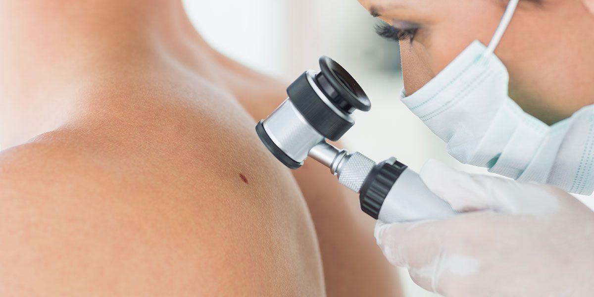
{"cells":[{"metadata":{},"cell_type":"markdown","source":"# **Melanoma Detection Using EfficientNet and MetaData Ensemble** <br>\nAuthor: TeYang, Lau<br>\nCreated: 1/5/2020<br>\nLast update: 17/8/2020<br>\n\n<img src = 'https://www.norrisderm.com/app/uploads/2013/06/portland-basal-cell-carcinoma-1200x600.jpg' width=\"700\">\n<br>\n\nThis notebook was created to try out **tensor processing unit** (TPU) for deep learning. TPU is developed by Google for neural network machine learning using Tensorflow, providing very high accuracy and speed. GPUs, on the other hand, have been around for a long time, and excel at matrix multiplication and parallelization, compared to CPUs. Although TPUs are more expensive than GPUs on a per hour basis, the time saved when training the same model will actually make it more cost-efficient when using a TPU. \n\nHere, I am using **EfficientNet** (EffNet) via **transfer learning**, one of the latest deep learning neural network model, to detect melanoma from images of skin lesions. This dataset consists of around 33,000 and 10,000 images in the training and testing set respectively. By leveraging the power of transfer learning, we are able to 'transfer' the weights of low-level features (e.g., lines, shapes, etc) that were detected in a pretrained model. Doing so saves us the need to train a model from scrach, which can be challenging for those who do not have a 'big' enough dataset or computational resources. I will also be trying out **Test Time Augmentation** to reduce errors for validation and test predictions. This will be explained further below.\n\nThis notebook uses code from [Chris Deotte's](https://www.kaggle.com/cdeotte) excellent [notebook](https://www.kaggle.com/cdeotte/triple-stratified-kfold-with-tfrecords) with some adjustments. All credits go to him!\n\nThe process is as follows:\n1. [Data Loading and Structure](#Data_loading_structure)\n2. [Set Up TPU](#TPU)\n3. [Setting Hyperparameters](#Hyperparameters)\n    - [Learning Rate Train Schedule](#TrainSchedule)\n4. [Image Loading Functions](#ImageLoading)\n5. [Train and Evaluate Model](#Train_model)\n    - [EfficientNets](#EffNets)\n    - [Test Time Augmentation](#TTA) \n    - [Out of Fold (OOF) in K-Fold Cross Validation](#OOF)\n    - [Label Smoothing](#LabelSmooth)\n    - [Calculate OOF AUC](#OOF_AUC)\n    - [ROC and PR Curves](#AUROC_AUPRC)\n6. [Predicting on Test Set](#Predict_test)\n7. [Meta-Data Train and Prediction](#MetaData) \n    - [Clean Train and Test Sets](#Clean)\n    - [Dummy Encoding](#Dummy)\n    - [Prepare Train and Test Sets](#Prepare)\n    - [Train, Predict and Blend](#TrainPredict)\n8. [Ensemble Model](#Ensemble)\n9. [Conclusion](#Conclusion)<br><br>\n","execution_count":null},{"metadata":{},"cell_type":"markdown","source":"Before we begin, let's watch a short video to get an idea of how melanoma is diagnosed!","execution_count":null},{"metadata":{"_kg_hide-input":true,"trusted":true},"cell_type":"code","source":"from IPython.display import YouTubeVideo,HTML\nYouTubeVideo(\"hXYd0WRhzN4\", width=700, height=500)","execution_count":null,"outputs":[]},{"metadata":{},"cell_type":"markdown","source":"<a id='Data_loading_structure'></a>\n# 1. Data Loading and Structure\n\nWe start by loading the dependencies and data, and exploring the dataset to look at its structure and distribution. We also print some images to get a hang of it.","execution_count":null},{"metadata":{"_uuid":"8f2839f25d086af736a60e9eeb907d3b93b6e0e5","_cell_guid":"b1076dfc-b9ad-4769-8c92-a6c4dae69d19","trusted":true},"cell_type":"code","source":"# import modules\n\nimport numpy as np \nimport pandas as pd \nimport math\nimport os\nimport glob\nimport matplotlib.pyplot as plt\nimport seaborn as sns\nimport PIL\n\nfrom sklearn import model_selection\nfrom sklearn.model_selection import KFold, StratifiedKFold, train_test_split\nfrom sklearn.model_selection import cross_validate, cross_val_score, GridSearchCV\nfrom sklearn.metrics import roc_auc_score\nfrom sklearn import model_selection\nfrom sklearn.metrics import confusion_matrix\nfrom mlxtend.plotting import plot_confusion_matrix\n\nfrom random import choices\nfrom functools import partial\nimport re\nfrom kaggle_datasets import KaggleDatasets\n\nimport tensorflow as tf\nimport tensorflow.keras.backend as K\nfrom tensorflow.keras.layers import Dense \nfrom tensorflow.keras.models import Model,Sequential\nfrom tensorflow.keras import optimizers\nfrom keras.utils.vis_utils import plot_model\n\n!pip install -q efficientnet\nimport efficientnet.tfkeras as efn\n","execution_count":null,"outputs":[]},{"metadata":{},"cell_type":"markdown","source":"This datasets that we will be using has been preprocessed for Tensorflow by [Chris Deotte](https://www.kaggle.com/cdeotte). The images have been resized and stored in tensorflow records (TFRecords), which will be more efficient when using TPU to load the images. Furthermore, the images have been triple stratified:\n1. All images from one patient are fully contained in a single TFRecord\n2. All TFRecords have equal data class proportion (i.e. each TFRecord now contains 1.8% malignant images)\n3. Each TFRecord has an equzal number of patients with 115 images, with 100 images, with 70 and so on.\n\nRefer to Chris's [post](https://www.kaggle.com/c/siim-isic-melanoma-classification/discussion/165526) for more information.","execution_count":null},{"metadata":{"_uuid":"d629ff2d2480ee46fbb7e2d37f6b5fab8052498a","_cell_guid":"79c7e3d0-c299-4dcb-8224-4455121ee9b0","trusted":true},"cell_type":"code","source":"train = pd.read_csv('/kaggle/input/siim-isic-melanoma-classification/train.csv')\n\ntest = pd.read_csv('/kaggle/input/siim-isic-melanoma-classification/test.csv')\n\nsample = pd.read_csv('/kaggle/input/siim-isic-melanoma-classification/sample_submission.csv')\n\ntrain.head()","execution_count":null,"outputs":[]},{"metadata":{"trusted":true},"cell_type":"code","source":"# look at distribution\n\nfig = plt.figure(figsize=(14,15))\n\nax1 = fig.add_subplot(321)\nax = train['benign_malignant'].value_counts().plot(kind='barh', color=['blue','red'], alpha=.5,\n                                                  title='Melanoma Target Distribution')\n\nax2 = fig.add_subplot(322)\nax2 = train['sex'].value_counts().plot(kind='barh', color=['blue','red'], alpha=.5,\n                                                  title='Sex Distribution')\n\nax3 = fig.add_subplot(323)\nax3 = train['diagnosis'].value_counts().plot(kind='barh', color=['blue','red'], alpha=.5,\n                                                  title='Diagnosis Distribution')\n\nax4 = fig.add_subplot(324)\nax4 = train['anatom_site_general_challenge'].value_counts().plot(kind='barh', \n                                                            color=['blue','red'], alpha=.5, \n                                                            title='Anatomical Site Distribution')\n\nax5 = fig.add_subplot(325)\nax5 = sns.distplot(train['age_approx'], kde=False)\n","execution_count":null,"outputs":[]},{"metadata":{},"cell_type":"markdown","source":"Notice that there are significantly more benign images compared to malignant images in the train dataset. Stratifying when splitting the train and validation set as well as during cross-validaton will thus be important. Another option is to apply some kind of weights to the loss so that the benign images will be weighted less.\n\nLet's look at some benign and malignant images. Can you identify the differences based on the video we just saw?","execution_count":null},{"metadata":{"_kg_hide-input":true,"trusted":true},"cell_type":"code","source":"%matplotlib inline \nfrom matplotlib.image import imread\nimport random\nimport cv2\n\n# Function for plotting samples\ndef plot_samples(samples):  \n    fig, ax = plt.subplots(nrows=4, ncols=5, figsize=(30,16))\n    for i in range(len(samples)):\n        image = imread(samples[i])\n        ax[i//5][i%5].imshow(image)\n        if i<10:\n            ax[i//5][i%5].set_title(\"Benign\", fontsize=20)\n        else:\n            ax[i//5][i%5].set_title(\"Malignant\", fontsize=20)\n        ax[i//5][i%5].axis('off')","execution_count":null,"outputs":[]},{"metadata":{"trusted":true},"cell_type":"code","source":"# sample images\n\ndirname = '/kaggle/input/siim-isic-melanoma-classification/jpeg/train/'\n# get benign filepaths \nsampleimg = [dirname + i + '.jpg' for i in train[train['benign_malignant'] == 'benign']['image_name'][:10]] + \\\n[dirname + i + '.jpg' for i in train[train['benign_malignant'] == 'malignant']['image_name'][:10]]\n\nplot_samples(sampleimg)\nplt.suptitle('Melanoma Samples', fontsize=30)\nplt.show()","execution_count":null,"outputs":[]},{"metadata":{},"cell_type":"markdown","source":"<a id='TPU'></a>\n# 2. Set Up TPU\n\nNow we set up the TPU so that training can be done faster. As the sizes of our models and datasets increase, we need to use either TPUs or GPUs to train our models within a reasonable amount of time. Built using 4 custom made ASICs or application-specific integrated circuit by Google specifically designed for machine learning using TensorFlow, TPUs offer a truly robust 180 TFLOPS of performance with 64GB of high bandwidth memory. This makes TPUs perfect for both training and inferencing of machine learning models.\n\n<img src=\"https://qph.fs.quoracdn.net/main-qimg-9ecde3fc6d69116db89aacd83bdf15e5\">","execution_count":null},{"metadata":{"trusted":true},"cell_type":"code","source":"AUTO = tf.data.experimental.AUTOTUNE\n\n# Detect hardware, return appropriate distribution strategy\ntry:\n    # TPU detection. No parameters necessary if TPU_NAME environment variable is set. \n    # On Kaggle this is always the case.\n    tpu = tf.distribute.cluster_resolver.TPUClusterResolver()  \n    print('Running on TPU ', tpu.master())\nexcept ValueError:\n    tpu = None\n\nif tpu:\n    tf.config.experimental_connect_to_cluster(tpu)\n    tf.tpu.experimental.initialize_tpu_system(tpu)\n    strategy = tf.distribute.experimental.TPUStrategy(tpu)\nelse:\n    # default distribution strategy in Tensorflow. Works on CPU and single GPU.\n    strategy = tf.distribute.get_strategy() \n\nREPLICAS = strategy.num_replicas_in_sync\nprint(\"REPLICAS: \", strategy.num_replicas_in_sync)\n","execution_count":null,"outputs":[]},{"metadata":{},"cell_type":"markdown","source":"<a id='Hyperparameters'></a>\n# 3. Setting Hyperparameters\n\nThe reason why there are multiple values for some of the hyperparameter is for training and experimenting with different models during each kfold. However, when training the final dataset, the hyperparameters should all be the same for all kfolds.","execution_count":null},{"metadata":{"trusted":true},"cell_type":"code","source":"# Hyperparameters\n\nSEED = 42\nFOLDS=3\nEFF_NETS = [6]*FOLDS\nBATCH_SIZES = [bs * strategy.num_replicas_in_sync for bs in [32]*FOLDS]\nIMG_SIZES = [512]*FOLDS\nEPOCHS = [10]*FOLDS\nDROPOUT = 0.25\nLR = 0.00004\nWARMUP = 5\n# CLASS WEIGHT SCALING\n# Scaling by total/2 helps keep the loss to a similar magnitude.\n# The sum of the weights of all examples stays the same.\nCLASS_WEIGHT = {0: train['benign_malignant'].value_counts().malignant/len(train),\n                1: train['benign_malignant'].value_counts().benign/len(train)}\n# WEIGHTS FOR FOLD MODELS WHEN PREDICTING TEST\nWGTS = [1/FOLDS]*FOLDS\nLABEL_SMOOTHING = 0.05\nTTA = 15 # test time augmentation\n\n# INCLUDE OLD COMP DATA? YES=1 NO=0\nINC2018 = [1]*FOLDS\n\n# seed\nnp.random.seed(SEED)\ntf.random.set_seed(SEED)","execution_count":null,"outputs":[]},{"metadata":{},"cell_type":"markdown","source":"Here, we set the paths to the different datasets containing different image sizes.","execution_count":null},{"metadata":{"trusted":true},"cell_type":"code","source":"# Get file paths for train, validation and test\n\nDATASET = {512: '512x512-melanoma-tfrecords-70k-images',\n           384: 'melanoma-384x384',\n           192: 'melanoma-192x192'}\n\nGCS_PATH = [None]*FOLDS; GCS_PATH2 = [None]*FOLDS\nfor i,k in enumerate(IMG_SIZES):\n    GCS_PATH[i] = KaggleDatasets().get_gcs_path(DATASET[IMG_SIZES[0]])\n    #GCS_PATH[i] = KaggleDatasets().get_gcs_path('melanoma-%ix%i'%(k,k))\n    GCS_PATH2[i] = KaggleDatasets().get_gcs_path('isic2019-%ix%i'%(k,k))\n\ntrain_filenames = tf.io.gfile.glob(GCS_PATH[0] + '/train*.tfrec')\n\ntest_filenames = tf.io.gfile.glob(GCS_PATH[0] + '/test*.tfrec')","execution_count":null,"outputs":[]},{"metadata":{},"cell_type":"markdown","source":"<a id='TrainSchedule'></a>\n### Learning Rate Train Schedule ###\n\nThis is a common train schedule for transfer learning. The learning rate starts near zero, then increases to a maximum, then decays over time. Consider changing the schedule and/or learning rates. Note how the learning rate max is larger with larger batches sizes. This is a good practice to follow.\n\nThe learning rate schedule we are using `get_lr_callback` is somewhat similar to the 1cycle learning rate policy. The 1cycle policy anneals the learning\nrate from an initial learning rate to some maximum learning rate and then from that maximum learning rate to some minimum learning rate much lower than the initial learning rate. This policy was initially described in the paper [Super-Convergence: Very Fast Training of Neural Networks Using Large Learning Rates](https://arxiv.org/abs/1708.07120). Refer to this [post](https://sgugger.github.io/the-1cycle-policy.html) to get a better understanding.","execution_count":null},{"metadata":{"trusted":true},"cell_type":"code","source":"def lrfn(epoch):\n    if epoch < lr_ramp_ep:\n        lr = (lr_max - lr_start) / lr_ramp_ep * epoch + lr_start\n\n    elif epoch < lr_ramp_ep + lr_sus_ep:\n        lr = lr_max\n\n    else:\n        lr = (lr_max - lr_min) * lr_decay**(epoch - lr_ramp_ep - lr_sus_ep) + lr_min\n\n    return lr\n\ndef get_lr_callback(batch_size=8):\n    lr_start   = 0.000005\n    lr_max     = 0.000003 * batch_size\n    lr_min     = 0.000001\n    lr_ramp_ep = 5\n    lr_sus_ep  = 0\n    lr_decay   = 0.3\n       \n    lr_callback = tf.keras.callbacks.LearningRateScheduler(lrfn, verbose=False)\n    return lr_callback","execution_count":null,"outputs":[]},{"metadata":{"trusted":true,"_kg_hide-input":true},"cell_type":"code","source":"lr_start   = 0.000005\nlr_max     = 0.000003 * BATCH_SIZES[0]\nlr_min     = 0.000001\nlr_ramp_ep = 5\nlr_sus_ep  = 0\nlr_decay   = 0.3\n\ndef lrfn(epoch):\n    if epoch < lr_ramp_ep:\n        lr = (lr_max - lr_start) / lr_ramp_ep * epoch + lr_start\n\n    elif epoch < lr_ramp_ep + lr_sus_ep:\n        lr = lr_max\n\n    else:\n        lr = (lr_max - lr_min) * lr_decay**(epoch - lr_ramp_ep - lr_sus_ep) + lr_min\n\n    return lr\n\nrng = [i for i in range(8 if EPOCHS[0]<8 else EPOCHS[0])]\ny = [lrfn(x) for x in rng]\nplt.plot(rng, y)\nprint(\"Learning rate schedule: {:.3g} to {:.3g} to {:.3g}\".format(y[0], max(y), y[-1]))","execution_count":null,"outputs":[]},{"metadata":{},"cell_type":"markdown","source":"<a id='ImageLoading'></a>\n# 4. Image Loading Functions\n\nHere we create some functions for loading TFRecords to get the images, target and image names.\n\n* **decode_image:** to transform images to a tensor, normalize it, and reshape it into the correct shape for TPU <br>\n* **read_tfrecord:** read the TFRecord, returns the image tensor, and based on the input arguments, return the label value, image name, or nothing (0) <br>\n* **load_dataset:** reads data from the TFRecords. Here we can choose whether to shuffle the data or not. We will do that for the train, but not the validation and test dataset.\n* **count_data_items:** counts the number of images in a file\n* **data_augment:** performs data augmentation\n* **plot_transform:** plots some examples of augmented images\n\n### Other augmentations\nHere we apply some manual augmentations that cannot be done with `tf.image`, such as shearing, zooming and translation. Rotation can be done in `tf.image` but only in factors of 90 degrees, so we do it manually instead.","execution_count":null},{"metadata":{"trusted":true,"_kg_hide-input":true},"cell_type":"code","source":"ROT_ = 180.0\nSHR_ = 2.0\nHZOOM_ = 8.0\nWZOOM_ = 8.0\nHSHIFT_ = 8.0\nWSHIFT_ = 8.0\n\ndef get_mat(rotation, shear, height_zoom, width_zoom, height_shift, width_shift):\n    # returns 3x3 transformmatrix which transforms indicies\n        \n    # CONVERT DEGREES TO RADIANS\n    rotation = math.pi * rotation / 180.\n    shear    = math.pi * shear    / 180.\n\n    def get_3x3_mat(lst):\n        return tf.reshape(tf.concat([lst],axis=0), [3,3])\n    \n    # ROTATION MATRIX\n    c1   = tf.math.cos(rotation)\n    s1   = tf.math.sin(rotation)\n    one  = tf.constant([1],dtype='float32')\n    zero = tf.constant([0],dtype='float32')\n    \n    rotation_matrix = get_3x3_mat([c1,   s1,   zero, \n                                   -s1,  c1,   zero, \n                                   zero, zero, one])    \n    # SHEAR MATRIX\n    c2 = tf.math.cos(shear)\n    s2 = tf.math.sin(shear)    \n    \n    shear_matrix = get_3x3_mat([one,  s2,   zero, \n                                zero, c2,   zero, \n                                zero, zero, one])        \n    # ZOOM MATRIX\n    zoom_matrix = get_3x3_mat([one/height_zoom, zero,           zero, \n                               zero,            one/width_zoom, zero, \n                               zero,            zero,           one])    \n    # SHIFT MATRIX\n    shift_matrix = get_3x3_mat([one,  zero, height_shift, \n                                zero, one,  width_shift, \n                                zero, zero, one])\n    \n    return K.dot(K.dot(rotation_matrix, shear_matrix), \n                 K.dot(zoom_matrix,     shift_matrix))\n\n\ndef transform(image, DIM=512):    \n    # input image - is one image of size [dim,dim,3] not a batch of [b,dim,dim,3]\n    # output - image randomly rotated, sheared, zoomed, and shifted\n    XDIM = DIM%2 #fix for size 331\n    \n    rot = ROT_ * tf.random.normal([1], dtype='float32')\n    shr = SHR_ * tf.random.normal([1], dtype='float32') \n    h_zoom = 1.0 + tf.random.normal([1], dtype='float32') / HZOOM_\n    w_zoom = 1.0 + tf.random.normal([1], dtype='float32') / WZOOM_\n    h_shift = HSHIFT_ * tf.random.normal([1], dtype='float32') \n    w_shift = WSHIFT_ * tf.random.normal([1], dtype='float32') \n\n    # GET TRANSFORMATION MATRIX\n    m = get_mat(rot,shr,h_zoom,w_zoom,h_shift,w_shift) \n\n    # LIST DESTINATION PIXEL INDICES\n    x   = tf.repeat(tf.range(DIM//2, -DIM//2,-1), DIM)\n    y   = tf.tile(tf.range(-DIM//2, DIM//2), [DIM])\n    z   = tf.ones([DIM*DIM], dtype='int32')\n    idx = tf.stack( [x,y,z] )\n    \n    # ROTATE DESTINATION PIXELS ONTO ORIGIN PIXELS\n    idx2 = K.dot(m, tf.cast(idx, dtype='float32'))\n    idx2 = K.cast(idx2, dtype='int32')\n    idx2 = K.clip(idx2, -DIM//2+XDIM+1, DIM//2)\n    \n    # FIND ORIGIN PIXEL VALUES           \n    idx3 = tf.stack([DIM//2-idx2[0,], DIM//2-1+idx2[1,]])\n    d    = tf.gather_nd(image, tf.transpose(idx3))\n        \n    return tf.reshape(d,[DIM, DIM,3])","execution_count":null,"outputs":[]},{"metadata":{"trusted":true},"cell_type":"code","source":"def decode_image(image):\n    # decode a JPEG-encoded image to a uint8 tensor\n    image = tf.image.decode_jpeg(image, channels=3) \n    # cast tensor to float32 and normalize to [0, 1] range\n    image = tf.cast(image, tf.float32)/255.0 \n    # explicit size needed for TPU\n    image = tf.reshape(image, [*IMG_SIZES[0:2], 3]) \n    return image\n\ndef read_tfrecord(example, labeled, return_imgname=False):\n    tfrecord_format = {\n        \"image\": tf.io.FixedLenFeature([], tf.string),\n        \"target\": tf.io.FixedLenFeature([], tf.int64)\n    } if labeled else {\n        \"image\": tf.io.FixedLenFeature([], tf.string),\n        \"image_name\": tf.io.FixedLenFeature([], tf.string)\n    }\n    example = tf.io.parse_single_example(example, tfrecord_format)\n    image = decode_image(example['image'])\n    # returns a dataset of (image, label) pairs if labeled=True\n    if labeled:\n        label = tf.cast(example['target'], tf.int32)\n        return image, label\n    idnum = example['image_name']\n    # returns a dataset of (image, image_name) pairs if return_imgname=True\n    if return_imgname:\n        return image, idnum\n    # else returns a dataset of (image, 0) pairs \n    return image, 0\n\ndef load_dataset(filenames, labeled=True, ordered=False, return_imgname=False):\n    # Read from TFRecords. For optimal performance, reading from multiple files at once and\n    # disregarding data order. Order does not matter since we will be shuffling the data anyway\n    ignore_order = tf.data.Options()\n    if not ordered:\n        ignore_order.experimental_deterministic = False # disable order, increase speed\n    # automatically interleaves reads from multiple files\n    dataset = tf.data.TFRecordDataset(filenames, num_parallel_reads=AUTO) \n    # uses data as soon as it streams in, rather than in its original order\n    dataset = dataset.with_options(ignore_order) \n    dataset = dataset.map(partial(read_tfrecord, labeled=labeled, \n                                  return_imgname=return_imgname), num_parallel_calls=AUTO)\n    , or (image, id) pairs if labeled=False\n    return dataset\n\ndef count_data_items(filenames):\n    n = [int(re.compile(r\"-([0-9]*)\\.\").search(filename).group(1)) for filename in filenames]\n    return np.sum(n)\n\ndef data_augment(image, label=None, seed=SEED):\n    # data augmentation. Thanks to the dataset.prefetch(AUTO) statement when \n    # loading dataset (below cell), this happens essentially for free on TPU. Data pipeline\n    # code is executed on the \"CPU\" part of the TPU while the TPU itself is \n    # computing gradients.\n    image = transform(image, IMG_SIZES[0])\n    #image = tf.image.rot90(image,k=np.random.randint(4)) # rotate\n    image = tf.image.random_flip_left_right(image, seed=seed) # flip horizontal\n    image = tf.image.random_flip_up_down(image, seed=seed) # flip vertical\n    image = tf.image.random_brightness(image, max_delta=0.2) # random brightness\n    image = tf.image.random_contrast(image, 0.8, 1.2) # random contrast\n    image = tf.image.random_saturation(image, 0.7, 1.3) # random saturation\n    \n    if label is None:\n        return image\n    else:\n        return image, label\n\n# plot augmented images sample\ndef plot_transform(num_images):\n    fig, ax = plt.subplots(nrows=3, ncols=num_images, figsize=(12,5))\n    x = (load_dataset(train_filenames, labeled=True)\n                     .shuffle(SEED)\n                     .batch(BATCH_SIZES[0],drop_remainder=True)                 \n                     .prefetch(AUTO)\n                     .unbatch().take(5))\n    images = []\n    imgs=[]\n    for r in range(3):\n        image,_ = iter(x).next()\n        images.append(image)\n        for i in range(0,num_images):\n            image = data_augment(image=images[r])\n            imgs.append(image)\n    for img in range(len(imgs)):          \n        ax[img//num_images][img%num_images].imshow(imgs[img])\n        ax[img//num_images][img%num_images].axis('off')","execution_count":null,"outputs":[]},{"metadata":{},"cell_type":"markdown","source":"Let's test out the functions to make sure they are working.","execution_count":null},{"metadata":{"trusted":true},"cell_type":"code","source":"# Function for plotting images in grid\ndef show_dataset(thumb_size, cols, rows, ds):\n    mosaic = PIL.Image.new(mode='RGB', size=(thumb_size*cols + (cols-1), \n                                             thumb_size*rows + (rows-1)))\n   \n    for idx, data in enumerate(iter(ds)):\n        img, target_or_imgid = data\n        ix  = idx % cols\n        iy  = idx // cols\n        img = np.clip(img.numpy() * 255, 0, 255).astype(np.uint8)\n        img = PIL.Image.fromarray(img)\n        img = img.resize((thumb_size, thumb_size), resample=PIL.Image.BILINEAR)\n        mosaic.paste(img, (ix*thumb_size + ix, \n                           iy*thumb_size + iy))\n\n    display(mosaic)\n    \neg_ds = (load_dataset(train_filenames, labeled=True)\n                     .batch(BATCH_SIZES[0],drop_remainder=True)                 \n                     .prefetch(AUTO)\n                     .unbatch().take(10*6))  \n\nshow_dataset(64, 10, 6, eg_ds)","execution_count":null,"outputs":[]},{"metadata":{},"cell_type":"markdown","source":"Here are some examples of the image augmentations","execution_count":null},{"metadata":{"trusted":true},"cell_type":"code","source":"plot_transform(7)","execution_count":null,"outputs":[]},{"metadata":{},"cell_type":"markdown","source":"<a id='Train_model'></a>\n# 5. Train and Evaluate Model\n\nBefore we train the model, let's take a moment to go through some of the concepts.\n\n<a id='EffNets'></a>\n### EfficientNets ###\n\nHere is a quick explanation of **EfficientNets**. \n\nIn training convolutional neural networks (CNNs), **scaling** is usually done to improve the model's accuracy, but it can also help in improving the efficiency of a model (i.e. how quickly it trains). There are three scaling dimensions of a CNN: *depth*, *width*, and *resolution*. **Depth** refers to how deep the networks is which is equivalent to the number of layers in it. **Width** refers to how wide the network is. One measure of width, for example, is the number of channels in a Conv layer whereas **Resolution** is simply the image resolution that is being passed to a CNN. \n\nHere is a picture showing the different scalings applied to a CNN:\n\n<img src=\"https://miro.medium.com/max/700/1*xQCVt1tFWe7XNWVEmC6hGQ.png\">\n\n<br>\n\nWhile depth scaling can allow a network to learn more complex and richer features, there is usually a diminishing return as the depth gets too large due to vanishing gradients, even when using techniques such as skip-connections in **Residual Networks**. Width scaling on the other hand allows models to be small and wider networks tend to capture more fine-grained features and are faster to train since they are smaller. However, performance again suffers with larger width. Resolution scaling is quite intuitive. Using larger resolutions is always better but the relationship is not linear. Therefore, ***scaling up any dimension of network (width, depth or resolution) improves accuracy, but the accuracy gain diminishes for bigger models.***\n\nEfficientNet was created with the idea of using **Compound Scaling**. This uses a **compound coefficient ɸ** to uniformly scale the network width, depth and resolution. ɸ is a user-specified coefficient, which produces **EfficientNets** ***B1-B7***. Refer to this [post](https://medium.com/@nainaakash012/efficientnet-rethinking-model-scaling-for-convolutional-neural-networks-92941c5bfb95) for a better intuition behind the scaling of EfficientNets.","execution_count":null},{"metadata":{},"cell_type":"markdown","source":"<a id='TTA'></a>\n### Test Time Augmentation ###\nSimilar to what Data Augmentation is doing to the training set, the purpose of **Test Time Augmentation** (TTA) is to perform random modifications to the test images. Instead of using the trained model to make a prediction on the *cleaned* and *original* test images, we augment the images several times, make a prediction on each of them, and get the average of each corresponding image. This will be the final prediction for that image. The reason why TTA works is that by averaging our predictions, we are also ***averaging the errors***. We can also apply TTA to the validation dataset to get a better performance on the validation set.\n\nRefer to this [post](https://towardsdatascience.com/test-time-augmentation-tta-and-how-to-perform-it-with-keras-4ac19b67fb4d) for a better intuition and examples of TTA.","execution_count":null},{"metadata":{},"cell_type":"markdown","source":"<a id='OOF'></a>\n### Out of Fold (OOF) in K-Fold Cross Validation ###\n\nIt is common to evaluate the performance of a machine learning algorithm on a dataset using a resampling technique such as k-fold cross-validation.\n\nThe k-fold cross-validation procedure involves splitting a training dataset into k groups, then using each of the k groups of examples on a validation set (hold out set/out of fold set) while the remaining examples are used as a training set. This means that k different models are trained and evaluated. The performance of the model is estimated using the predictions by the models made across all k-folds.\n\nAn **out-of-fold (OOF)** prediction is a prediction by the model during the k-fold cross-validation procedure. That is, out-of-fold predictions are those predictions made on the holdout datasets during the resampling procedure. If performed correctly, there will be one prediction for each example in the training dataset.","execution_count":null},{"metadata":{},"cell_type":"markdown","source":"<a id='LabelSmooth'></a>\n### Label Smoothing ###\n\nLabel smoothing is a regularization technique for classification problems to prevent the model from predicting the training examples too confidently, thus improving the robustness of the model to generalize well. In classification, the softmax function is usually applied to the penultimate layer's logit vectors to compute its output probabilities. The problem with using hard targets (e.g., [1,0,0,0] for one-hot encoding) in classification is that they encourage the largest logit gaps to be fed into the softmax function, which results in a model that is ***too confident*** about its predictions. This can also lead to overfitting.\n\nLabel smoothing attempts to overcome this by applying a smoothing parameter `α` to modify the targets into softer targets, thus reducing the gap between the largest logit and the rest. Refer to this [post](https://towardsdatascience.com/what-is-label-smoothing-108debd7ef06) and this [post](https://medium.com/@nainaakash012/when-does-label-smoothing-help-89654ec75326) for a more in-depth discussion.","execution_count":null},{"metadata":{},"cell_type":"markdown","source":"Finally, let's train and evaluate the model. Notice that for the prediction on the test set, we are using each fold's best model to predict on the entire test set. The predictions are then averaged across the number of folds (through the `WGTS` hyperparameter, which is set as 1/fold). ","execution_count":null},{"metadata":{"trusted":true},"cell_type":"code","source":"# USE VERBOSE=0 for silent, VERBOSE=1 for interactive, VERBOSE=2 for commit\nVERBOSE = 2\nDISPLAY_PLOT = True\n\nskf = KFold(n_splits=FOLDS,shuffle=True,random_state=SEED)\n# initialize for out of fold storage\noof_pred = []; oof_tar = []; oof_val = []; oof_names = []; oof_folds = [] \n# initialize for prediction storage\npreds = np.zeros((count_data_items(test_filenames),1))                    \n\n# idxT=train tfrec num, idxV=val tfrec num\n# loop through the kfolds and get the stratified sets\nfor fold,(idxT,idxV) in enumerate(skf.split(np.arange(15))):\n    \n    if tpu: tf.tpu.experimental.initialize_tpu_system(tpu) # initialize TPU\n          \n    # CREATE TRAIN, VALIDATION & TEST SETS FOR CURRENT FOLD\n    # get the files in the stratified fold\n    files_train = tf.io.gfile.glob([GCS_PATH[fold] + '/train%.2i*.tfrec'%x for x in idxT]) \n    # include 2018 comp data\n    if INC2018[fold]:\n        files_train += tf.io.gfile.glob([GCS_PATH2[fold] + '/train%.2i*.tfrec'%x for x in idxT*2])\n    np.random.seed(SEED)\n    np.random.shuffle(files_train); print('#'*25)   # shuffle training set\n    train_dataset = (load_dataset(files_train, labeled=True)\n                     .repeat()                      # repeat to continue getting data for aug\n                     .map(data_augment, num_parallel_calls=AUTO)\n                     .shuffle(SEED)\n                     .batch(BATCH_SIZES[fold],drop_remainder=True)\n                     # prefetch next batch while training (autotune prefetch buffer size)\n                     .prefetch(AUTO)) \n    files_valid = tf.io.gfile.glob([GCS_PATH[fold] + '/train%.2i*.tfrec'%x for x in idxV])\n    files_test = np.sort(np.array(tf.io.gfile.glob(GCS_PATH[fold] + '/test*.tfrec')))\n\n          \n    # BUILD MODEL\n    # when creating multiple models during CV, each model adds nodes to the graph,\n    # best to clear the nodes to prevent memory hogging, which slows down training\n    K.clear_session()\n    with strategy.scope():\n        model = tf.keras.Sequential([\n            efn.EfficientNetB6(input_shape=(IMG_SIZES[fold],IMG_SIZES[fold], 3),\n                               weights='imagenet',pooling='avg',include_top=False),\n        # add fully connected layer, with sigmoid activation since only 2 categories\n            Dense(1, activation='sigmoid') \n        ])\n        model.compile(\n            optimizer='adam',\n            loss = tf.keras.losses.BinaryCrossentropy(label_smoothing = LABEL_SMOOTHING),\n            metrics=[tf.keras.metrics.AUC(name='auc')])\n    \n    # for saving best model from the best epoch in each kfold\n    sv = tf.keras.callbacks.ModelCheckpoint(\n            'fold-%i.h5'%fold, monitor='val_loss', verbose=0, save_best_only=True,\n            save_weights_only=True, mode='min', save_freq='epoch')\n\n    # DISPLAY FOLD INFO\n    print('#'*25); print('#### FOLD',fold+1)\n    print('#### Image Size %i with EfficientNet B%i and batch_size %i'%\n          (IMG_SIZES[fold],EFF_NETS[fold],BATCH_SIZES[fold]))\n    \n    # TRAIN\n    print('Training...')         \n    history = model.fit(\n        train_dataset, \n        epochs=EPOCHS[fold], \n        callbacks=[sv,get_lr_callback(BATCH_SIZES[fold])],                      # lr schedule\n        steps_per_epoch=count_data_items(files_train) // BATCH_SIZES[fold],\n        validation_data=load_dataset(files_valid, labeled=True)                                        \n                         .cache()\n                         .batch(BATCH_SIZES[fold])\n                         .prefetch(AUTO),\n        #class_weight=CLASS_WEIGHT,                                             # class weights\n        verbose=VERBOSE)\n    \n    # LOAD BEST MODEL\n    print('Loading best model...')\n    model.load_weights('fold-%i.h5'%fold)\n    \n    # PREDICT OOF USING TTA\n    print('Predicting OOF with TTA...')\n    ds_valid = (load_dataset(files_valid, labeled=True, ordered=True)                                        \n                     .cache()     \n                     .repeat()                              # repeat for data aug during oof val\n                     .map(data_augment, num_parallel_calls=AUTO)  # data augmentation \n                     .batch(BATCH_SIZES[fold]*4)            # X4 to speed up training\n                     .prefetch(AUTO))\n    ct_valid = count_data_items(files_valid)\n    STEPS = TTA * ct_valid/BATCH_SIZES[fold]/4    #number of steps to go through all TTA images\n    # slice to throw away images that pass the steps\n    pred = model.predict(ds_valid,steps=STEPS,verbose=VERBOSE)[:TTA*ct_valid,] \n    # store the average of each valid image\n    oof_pred.append( np.mean(pred.reshape((ct_valid,TTA),order='F'),axis=1) ) \n    \n    # GET OOF TARGETS, FOLDS, AND NAMES\n    # get targets\n    # do not repeat=True here as we only want the target values\n    ds_valid = (load_dataset(files_valid, labeled=True, ordered=True) # do not shuffle\n                        .cache()\n                        .batch(BATCH_SIZES[fold]*4)\n                        .prefetch(AUTO))\n    oof_tar.append( np.array([target.numpy() for img, target in iter(ds_valid.unbatch())]) )\n    # track which fold data comes from\n    oof_folds.append( np.ones_like(oof_tar[-1],dtype='int8')*fold ) \n    # get names\n    ds = (load_dataset(files_valid, labeled=False, return_imgname=True, ordered=True)                                        \n                .cache()     \n                .batch(BATCH_SIZES[fold]*4)                   \n                .prefetch(AUTO))\n    oof_names.append( np.array([img_name.numpy().decode(\"utf-8\") for img, img_name in iter(ds.unbatch())]))      \n          \n    # PREDICT TEST USING TTA\n    print('Predicting Test with TTA...')\n    ds_test = (load_dataset(files_test, labeled=False, ordered=True) # do not shuffle\n              .repeat()                                              # repeat for TTA\n              .map(data_augment, num_parallel_calls=AUTO)            # data augmentation \n              .batch(BATCH_SIZES[fold]*4)\n              .prefetch(AUTO))\n    ct_test = count_data_items(files_test)\n    STEPS = TTA * ct_test/BATCH_SIZES[fold]/4 #number of steps to go through all TTA images\n    # slice to throw away images that pass the steps\n    pred = model.predict(ds_test,steps=STEPS,verbose=VERBOSE)[:TTA*ct_test,] \n    # store the average pred of each test image\n    preds[:,0] += np.mean(pred.reshape((ct_test,TTA),order='F'),axis=1) * WGTS[fold] \n    \n    # REPORT RESULTS\n    auc = roc_auc_score(oof_tar[-1],oof_pred[-1])\n    oof_val.append(np.max( history.history['val_auc'] ))\n    print('#### FOLD %i OOF AUC without TTA = %.3f, with TTA = %.3f'%(fold+1,oof_val[-1],auc))\n          \n    # PLOT TRAINING AND VALIDATION\n    if DISPLAY_PLOT:\n        plt.figure(figsize=(15,5))\n        plt.plot(np.arange(EPOCHS[fold]),history.history['auc'],'-o',\n                 label='Train AUC',color='#ff7f0e')\n        plt.plot(np.arange(EPOCHS[fold]),history.history['val_auc'],'-o',\n                 label='Val AUC',color='#1f77b4')\n        x = np.argmax( history.history['val_auc'] ); y = np.max( history.history['val_auc'] )\n        xdist = plt.xlim()[1] - plt.xlim()[0]; ydist = plt.ylim()[1] - plt.ylim()[0]\n        plt.scatter(x,y,s=200,color='#1f77b4')\n        plt.text(x-0.03*xdist,y-0.13*ydist,'max auc\\n%.2f'%y,size=14)\n        plt.ylabel('AUC',size=14); plt.xlabel('Epoch',size=14)\n        plt.legend(loc=2)\n        plt2 = plt.gca().twinx()\n        plt2.plot(np.arange(EPOCHS[fold]),history.history['loss'],'-o',\n                  label='Train Loss',color='#2ca02c')\n        plt2.plot(np.arange(EPOCHS[fold]),history.history['val_loss'],'-o',\n                  label='Val Loss',color='#d62728')\n        x = np.argmin( history.history['val_loss'] )\n        y = np.min( history.history['val_loss'] )\n        ydist = plt.ylim()[1] - plt.ylim()[0]\n        plt.scatter(x,y,s=200,color='#d62728')\n        plt.text(x-0.03*xdist,y+0.05*ydist,'min loss',size=14)\n        plt.ylabel('Loss',size=14)\n        plt.xticks(ticks=list(range(EPOCHS[fold])),labels=list(range(1, EPOCHS[fold]+1)))\n        plt.title('FOLD %i - Image Size %i, EfficientNet B%i, inc2018=%i'%\n                (fold+1,IMG_SIZES[fold],EFF_NETS[fold],INC2018[fold]),size=18)\n        plt.legend(loc=3)\n        plt.show()","execution_count":null,"outputs":[]},{"metadata":{},"cell_type":"markdown","source":"We can see that the validation and train AUC are quite close together, although on some folds, they start to diverge towards the end of the epochs, a sign that it might be overfitting.\n\nNevertheless, max performance seems to be ~0.9 AUC.","execution_count":null},{"metadata":{},"cell_type":"markdown","source":"<a id='OOF_AUC'></a>\n### Calculate OOF AUC ###\n\nHere we calculate the out-of-fold AUC for all train data to get an idea of the overall validation performance.","execution_count":null},{"metadata":{"trusted":true},"cell_type":"code","source":"# COMPUTE OVERALL OOF AUC\noof = np.concatenate(oof_pred); true = np.concatenate(oof_tar);\nnames = np.concatenate(oof_names); folds = np.concatenate(oof_folds)\nauc = roc_auc_score(true,oof)\nprint('Overall OOF AUC with TTA = %.3f'%auc)\n\n# SAVE OOF TO DISK\ndf_oof = pd.DataFrame(dict(\n    image_name = names, target=true, pred = oof, fold=folds))\ndf_oof.to_csv('oof.csv',index=False)\ndf_oof.head()","execution_count":null,"outputs":[]},{"metadata":{},"cell_type":"markdown","source":"<a id='AUROC_AUPRC'></a>\n### ROC and PR Curves ###\n\nLet's plot out the area under receiver operating characteristic curve (AUROC) and the area under precision recall curve (AUPRC). When there is a high imalance in the classes, in this case - number of benign greatly exceeds the number of malignant images, the AUROC may give a over-optimistic view of the performance of the model and the AUPRC might be better. \n\nFor example, a big improvement in the number of false positives only leads to a small change in the false positive rate when using ROC. Precision, on the other hand, by comparing false positives to true positives rather than true negatives, captures the effect of the large number of negative examples on the model’s performance. \n\nRefer to this paper titled [The Relationship Between Precision-Recall and ROC Curves](http://pages.cs.wisc.edu/~jdavis/davisgoadrichcamera2.pdf) for a great explanation of the relationship.\n\n**More on Precision and Recall:**<br>\n**Accuracy** is not a good evaluation metric when there is huge **data class imbalance**. Imagine that if we have 100 samples: 99 pneumonia and 1 normal, then a model that predicts everything as pneumonia will get an accuracy of 99%. In this case, its better to look at **precision and recall**, and their harmonic mean, the **F1 score**. \n\nThis can be visualized using a confusion matrix as well.\n\n<img src = 'https://bk9zeg.bn.files.1drv.com/y4mZtoVgcWgAYE59g3lpWQ3PaZWMqnDN7gz1ir2LIgyPjR6a26Ij1vDBmjsETpEmvAkebvyLjSVofcRVSjW8Ux62r8_tIyIK6AZJ7GQOz_sWtAj_hdQIA57pbJaEpHJEeY_pG7odhdU1osvM7jHXfFzpVsIOt76oqNe39j4KZIFRDOguHUr5jPtDe0TIzNTLQuehcuQdw-aIjt7FR9D6Ti9-A?width=618&height=419&cropmode=none' width=\"600\">\n\n<br>\nSince this competition has a huge class imbalance, with more benign than malignant images, it makes more sense to use a AUPRC but the competition states to use AUROC. However, we will plot out both. We can see that the PRC shows that there can still be lots of improvement to the model while the ROC curve gives a over-optimistic view of how our model is performing. <br>\n\n<br>\n\nThis paper titled [The Relationship Between Precision-Recall and ROC Curves](http://pages.cs.wisc.edu/~jdavis/davisgoadrichcamera2.pdf) provides a great explanation of the relationship between ROC and PRC.\n\nMore resources here: [The Precision-Recall Plot Is More Informative than the ROC Plot When Evaluating Binary Classifiers on Imbalanced Datasets](https://journals.plos.org/plosone/article?id=10.1371/journal.pone.0118432).\n","execution_count":null},{"metadata":{"_kg_hide-input":true,"trusted":true},"cell_type":"code","source":"from sklearn.metrics import roc_curve, auc, precision_recall_curve, average_precision_score\n\n# AUROC\nfpr = dict()\ntpr = dict()\nroc_auc = dict()\nfor i in range(FOLDS):\n    fpr[i], tpr[i], _ = roc_curve(df_oof[df_oof.fold==i].target, df_oof[df_oof.fold==i].pred)\n    roc_auc[i] = auc(fpr[i], tpr[i])\nfpr[\"mean\"], tpr[\"mean\"], _ = roc_curve(df_oof.target, df_oof.pred)\nroc_auc['mean'] = auc(fpr['mean'], tpr['mean'])\n\n# AUPRC\nprecision = dict()\nrecall = dict()\naverage_precision = dict()\nfor i in range(FOLDS):\n    precision[i], recall[i], _ = precision_recall_curve(df_oof[df_oof.fold==i].target, \n                                                        df_oof[df_oof.fold==i].pred)\n    average_precision[i] = average_precision_score(df_oof[df_oof.fold==i].target, \n                                                        df_oof[df_oof.fold==i].pred)\nprecision[\"mean\"], recall[\"mean\"], _ = precision_recall_curve(df_oof.target, df_oof.pred)\naverage_precision['mean'] = average_precision_score(df_oof.target, df_oof.pred)\n\n# PLOT\n# auroc\nfig = plt.figure(figsize=(18,6))\nax1 = fig.add_subplot(121)\n\nax1.plot([0, 1], [0, 1], linestyle='--', lw=4, color='r',\n        label='Chance', alpha=.8)\n\ncolors = ['#1f77b4', '#ff7f0e', '#2ca02c', '#d62728', '#9467bd',\n          '#8c564b', '#e377c2', '#7f7f7f', '#bcbd22', '#17becf']\nfor i in range(FOLDS):\n    ax1.plot(fpr[i], tpr[i], color=colors[i],\n        label=r'ROC Fold %i (AUC = %0.2f)' % (i+1,roc_auc[i]),\n        lw=3, alpha=.5)\n\nax1.plot(fpr['mean'], tpr['mean'], color='b',\n        label=r'Mean ROC (AUC = %0.2f)' % (roc_auc['mean']),\n        lw=4, alpha=.8)    \n    \nax1.set(xlim=[-0.05, 1.05], ylim=[-0.05, 1.05])\nplt.title(\"Receiver Operating Characteristic Curve\", size=25)\nplt.xlabel('False Positive Rate',size=20); plt.xticks(size=15)\nplt.ylabel('True Positive Rate',size=20); plt.yticks(size=15)\nax1.legend(loc=\"lower right\",prop={\"size\":15})\n\n# auprc\nax2 = fig.add_subplot(122)\nfor i in range(FOLDS):\n    ax2.step(recall[i], precision[i], where='post', color=colors[i],\n             label=r'AP Fold %i (AP = %0.2f)' % (i+1,average_precision[i]),\n             lw=3, alpha=.5)\n\nax2.step(recall['mean'], precision['mean'], where='post', color='b',\n        label=r'Mean AP (AP = %0.2f)' % (average_precision['mean']),\n        lw=4, alpha=.8)    \n    \nax2.set(xlim=[-0.05, 1.05], ylim=[-0.05, 1.05])\nplt.title(\"Precision Recall Curve\", size=25)\nplt.xlabel('Recall',size=20); plt.xticks(size=15)\nplt.ylabel('Precision',size=20); plt.yticks(size=15)\nax2.legend(loc=\"lower left\",prop={\"size\":15})\n\nplt.show()","execution_count":null,"outputs":[]},{"metadata":{},"cell_type":"markdown","source":"<a id='Predict_test'></a>\n# 6. Test Set Predictions\n\nLet's gather the test set predictions and organize them into a dataframe.","execution_count":null},{"metadata":{"trusted":true},"cell_type":"code","source":"test_ds = (load_dataset(files_test, labeled=False, return_imgname=True, ordered=True)\n              .batch(BATCH_SIZES[fold])\n              .prefetch(AUTO))\nimage_names = np.array([img_name.numpy().decode(\"utf-8\") \n                        for img, img_name in iter(test_ds.unbatch())])\n\nsubmission = pd.DataFrame(dict(image_name=image_names, target=preds[:,0]))\nsubmission = submission.sort_values('image_name').reset_index(drop=True) \nsubmission.to_csv('submission_noensemble.csv', index=False)\nsubmission.head()","execution_count":null,"outputs":[]},{"metadata":{"trusted":true},"cell_type":"code","source":"plt.hist(submission.target,bins=100)\nplt.show()","execution_count":null,"outputs":[]},{"metadata":{},"cell_type":"markdown","source":"<a id='MetaData'></a>\n# 7. Meta-Data Train and Prediction\n\nIn addition to the images themselves, they also come together with some meta-data. This include information like `age`, `sex` and `site of lesion`. We can train a weak model to predict melanoma based on these features, then blend the predictions together (ensemble) with the EffNet prediction. We will also need to apply some weightings to the predictions as the predictions from the meta-data are weak and should not contribute equally towards the final predictions.\n\nHere we are using the 2020 metadata together with past years' data.","execution_count":null},{"metadata":{},"cell_type":"markdown","source":"<a id='Clean'></a>\n### Clean Train and Test Sets ###\n\nHere we account for missing data. For `age`, we simply replace with the mean. For the categorical features `sex` and `anatom_site_general_challenge`, we replace missing values with a class level with probability proportional to the class distribution of the feature. For example for sex, if males made up 60% of the sample, then a missing value will be assigned as male 60% of the time. Since the external data have more detailed anatomical location classes than 2020, we will have to deal with them. All the different sites on the torso will be merged to just torso.","execution_count":null},{"metadata":{"trusted":true},"cell_type":"code","source":"train = pd.read_csv('/kaggle/input/melanomaextendedtabular/external_upsampled_tabular.csv')\ntrain.head()","execution_count":null,"outputs":[]},{"metadata":{"trusted":true},"cell_type":"code","source":"# marge different sites of torso to just torso\ntrain['anatom_site_general_challenge'].replace(['anterior torso','lateral torso','posterior torso'], \n                                               'torso', inplace=True)","execution_count":null,"outputs":[]},{"metadata":{"trusted":true},"cell_type":"code","source":"train.isnull().sum()","execution_count":null,"outputs":[]},{"metadata":{"trusted":true},"cell_type":"code","source":"def fillna(df, column):\n    na_idx = df[df[column].isnull()].index.tolist() # get idx of nulls\n    prob = df[column].value_counts(normalize=True).sort_index().tolist()\n    for i in na_idx:\n        df.iloc[i, df.columns.get_loc(column)] = choices(sorted(df[column].dropna().unique().tolist()), prob)[0]\n\ntrain.sex.replace('unknown', np.nan, inplace=True) # replace unknown sex with NaNs\nfillna(train, 'sex')\nfillna(train, 'anatom_site_general_challenge')   \nfillna(test, 'anatom_site_general_challenge')\n# replace null age with mean age\ntrain['age_approx'] = train['age_approx'].fillna(round(train['age_approx'].mean())) \n\n# Check missing data cleaning\nprint('Train Missing Data Count: %i, Test Missing Data Count: %i'%(train.isnull().sum().sum(), test.isnull().sum().sum()))","execution_count":null,"outputs":[]},{"metadata":{},"cell_type":"markdown","source":"<a id='Dummy'></a>\n### Dummy Encoding ###","execution_count":null},{"metadata":{"trusted":true},"cell_type":"code","source":"# dummy encode categorical features\ntrain = pd.get_dummies(train, columns=[\"anatom_site_general_challenge\"], prefix='site',\n                       drop_first=True)\ntrain.replace({'sex': {'female':0, 'male': 1}}, inplace=True)\n\ntrain.head()","execution_count":null,"outputs":[]},{"metadata":{"trusted":true},"cell_type":"code","source":"# dummy encode categorical features\ntest = pd.get_dummies(test, columns=[\"anatom_site_general_challenge\"], prefix='site',\n                      drop_first=True)\ntest.replace({'sex': {'female':0, 'male': 1}}, inplace=True)\ntest.head()","execution_count":null,"outputs":[]},{"metadata":{},"cell_type":"markdown","source":"<a id='Prepare'></a>\n### Prepare Train and Test Sets ###","execution_count":null},{"metadata":{"trusted":true},"cell_type":"code","source":"y_train = train['target']\nX_train = train.drop(['image_name','height','width','target'],\n                     axis=1)\nX_test = test.drop(['image_name','patient_id'],axis=1)\n\n# Scaling\nfrom sklearn.preprocessing import StandardScaler\n\nscaler = StandardScaler()\nX_train_s = X_train.copy()\nX_train_s[['age_approx']] = scaler.fit_transform(X_train_s[['age_approx']])\nX_test_s = X_test.copy()\nX_test_s[['age_approx']] = scaler.fit_transform(X_test_s[['age_approx']])\n\nX_train_s.head()","execution_count":null,"outputs":[]},{"metadata":{},"cell_type":"markdown","source":"<a id='TrainPredict'></a>\n### Train, Predict and Blend###\nWe will train 3 models using cross-validation then average their predictions.","execution_count":null},{"metadata":{"trusted":true},"cell_type":"code","source":"from sklearn.linear_model import LogisticRegression\nfrom sklearn.naive_bayes import GaussianNB\nfrom sklearn.ensemble import RandomForestClassifier\n\nlr = LogisticRegression(penalty='l2', class_weight='balanced', random_state=SEED)\nnb = GaussianNB()\nrf = RandomForestClassifier(n_estimators=1000, max_depth=2, class_weight='balanced',\n                            n_jobs=-1, random_state=SEED)\n\nestimators = [lr, rf, nb]\ncv = StratifiedKFold(5, shuffle=True, random_state=SEED)\n\ndef model_cv(X_train, y_train, estimators, cv):\n    \n    for est in estimators:\n        model_name = est.__class__.__name__\n        cv_results = cross_validate(est, X_train, y_train, cv=cv,\n                                scoring='roc_auc',\n                                return_train_score=True,\n                                n_jobs=-1)\n        train_score = cv_results['train_score'].mean()\n        test_score = cv_results['test_score'].mean()\n        \n        print('%s - Train Score: %.3f, Val Score: %.3f'%(model_name,train_score,test_score))\n        \n        \nmodel_cv(X_train_s, y_train, estimators, cv)","execution_count":null,"outputs":[]},{"metadata":{"trusted":true},"cell_type":"code","source":"# Predict and Blend\ndef model_blend(X_train, y_train, X_test, estimators):\n    mean_prob = 0\n    \n    for est in estimators:\n        est.fit(X_train, y_train)\n        mean_prob += est.predict_proba(X_test)[:,1]\n        \n    return mean_prob/len(estimators) # return the average\n\nmeta_df = pd.DataFrame(columns=['image_name', 'target'])\nmeta_df['image_name'] = sample['image_name']\n# predict and add to meta df\nmeta_df['target'] = model_blend(X_train_s, y_train, X_test_s, estimators)\n\nmeta_df.to_csv('meta_pred.csv', header=True, index=False)\nmeta_df.head()","execution_count":null,"outputs":[]},{"metadata":{},"cell_type":"markdown","source":"<a id='Ensemble'></a>\n# 8. Ensemble Model\n\nHere we assign the meta-data prediction a 0.1 weight while giving the majority of the weights to the EffNets. Here I uploaded the EffNets ensemble that I did outside of the notebook which consists of 6 models from EffNets B2,B4,B6 on 384 and 512 images. They have already been given equal weights of 0.15 (0.15 x 6 = 0.9).","execution_count":null},{"metadata":{"trusted":true},"cell_type":"code","source":"submission_effnet_ensemble = pd.read_csv('../input/effnet-ensemble/submission_effnet_ensemble.csv')\nsubmission.target = (submission_effnet_ensemble.target) + (meta_df.target * 0.1)\nsubmission.to_csv('submission.csv', index=False)\nsubmission.head()","execution_count":null,"outputs":[]},{"metadata":{},"cell_type":"markdown","source":"<a id='Conclusion'></a>\n# 9. Conclusion\n\nIn conclusion, our model performs reasonably well based on AUROC score but there can still be room for vast improvement according to the AUPRC score. In the diagnosis of melanoma (to classify lesions as malignant or benign), we often want our recall/sensitivity to be high since we want to correctly identify all true malignant cases. For our model, if we set a low threshold to get a high recall, our precision will greatly suffer, which means that during melanoma screening, many people will get false diagnosis of melanoma (high false positives). Therefore, the current model is still not great for deployment.\n\n**Below are some of the difficulties that I faced for this dataset:**\n\n* **Data class imbalance:** This is quite prevalent in the real world and as data scientists, we should all learn to embrace it and find ways to get around this problem. Usually, one way is to simply collect more data for the undersampled class. However, this is not possible for this dataset and especially for healthcare data, which is very difficult to collect and share. In reality, malignant cases will also be less prevalent than benign cases. In this notebook, I used stratified sampling to get around this problem but this does not totally solve the issue. One other way might be to apply weighted loss to give more weights to the loss of the malignant images. However, I tried it and it seems to hinder performance for this dataset. Here is a [post](https://www.tensorflow.org/tutorials/structured_data/imbalanced_data#class_weights) on some ways to deal with inbalanced datasets.\n\n* **Overfitting:** This dataset is prone to overfitting, especially if one uses a quickly increasing learning rate. Therefore, I only ran the model for ~ 8 epochs as it starts to overtrain by then.\n\n\n**What I learnt:**\n* **Learning rate scheduling using** [**One fit cycle:**](https://pytorch.org/docs/stable/_modules/torch/optim/lr_scheduler.html#OneCycleLR) The 1cycle policy anneals the learning rate from an initial learning rate to some maximum learning rate and then from that maximum learning rate to some minimum learning rate much lower than the initial learning rate. This policy was initially described in the paper [Super-Convergence: Very Fast Training of Neural Networks Using Large Learning Rates](https://arxiv.org/abs/1708.07120). Refer to this [post](https://sgugger.github.io/the-1cycle-policy.html) to get a better understanding.\n* **EfficientNets:** Who would have thought that such a simple scaling of the 3 dimensions of a CNN can lead to such efficiency in model training!\n* **Using TPUs:** TPUs are really efficient for training large neural networks and data compared to CPU and GPU. The future of deep learning and AI is becoming more impressive.   \n* **Test Time Augmentation:** TTA provides a way to reduce the errors in the predictions and is a really useful technique. Combined with TPU, it provides the opportunity to train and evaluate models with a lot more diversity in the data.\n* **Label Smoothing:** A useful regularization technique for preventing the model from predicting too confidently by modifying hard labels into soft labels, which reduces the gap between the largest logit and the rest.\n* **Kfold Cross Validation in Neural Networks:** For my past deep learning projects, I have always trained using a separate train and validation sets. K-fold CV provide a more robust way to evaluate the performance of the model, and it has the advantage that every image is trained and evaluated.  \n* **Using Ensemble models from different data:** Combining predictions trained from images using CNNs and metadata is a great way to improving the performance of the model.  ","execution_count":null},{"metadata":{},"cell_type":"markdown","source":"<font size=\"+3\" color=\"steelblue\"><b>My other works</b></font><br>\n\n<div class=\"row\">\n    \n  <div class=\"col-sm-4\">\n    <div class=\"card\">\n      <div class=\"card-body\" style=\"width: 20rem;\">\n         <h5 class=\"card-title\"><u>Pneumonia Detection with PyTorch</u></h5>\n         <img style='height:170' src=\"https://raw.githubusercontent.com/teyang-lau/Pneumonia_Detection/master/Pictures/train_grid.png\" class=\"card-img-top\" alt=\"...\"><br>\n         <p class=\"card-text\">Pneumonia Detection using Transfer Learning via ResNet in PyTorch</p>\n         <a href=\"https://www.kaggle.com/teyang/pneumonia-detection-resnets-pytorch\" class=\"btn btn-primary\" style=\"color:white;\">Go to Post</a>\n      </div>\n    </div>\n  </div>   \n    \n  <div class=\"col-sm-4\">\n    <div class=\"card\">\n      <div class=\"card-body\" style=\"width: 20rem;\" style='background:red'>\n        <h5 class=\"card-title\"><u>Neural Style Transfer</u></h5> <br>\n        <img style='width:300px' src=\"https://19qfnq.bn.files.1drv.com/y4moRovvJtBA5ccvsFv6iZadlO2ZxIOTXTof4On35sxnsKBLgN6bLHpfYsdl9CtqT4H8pcM_UjRNLqqtWKxf3FMhvAzdOg-I4-6UbA35rI6UMoHkCLxkpvc6iy-mqm_AoOdsWsbDy1ka8ek8a7kzHWjd-boIug4FyjCnAOtv4ipgLjP4XCXRgmv0qK1rKvB_I774lTJDqeQl_0v6jgZM3m-dA?width=829&height=469&cropmode=none\" class=\"card-img-top\" alt=\"...\"><br>\n        <p class=\"card-text\">Neural Style Transfer Using VGG19 to Create Artistic Pictures.</p>\n        <a href=\"https://www.kaggle.com/teyang/neural-style-transfer-for-unique-artistic-photos\" class=\"btn btn-primary\" style=\"color:white;\">Go to Post</a>\n      </div>\n    </div>\n  </div>\n    \n  <div class=\"col-sm-4\">\n    <div class=\"card\">\n      <div class=\"card-body\" style=\"width: 20rem;\">\n         <h5 class=\"card-title\"><u>Covid-19 & Google Trends</u></h5>\n         <img style='height:135px' src=\"https://miro.medium.com/max/821/1*Fi6masemXJT3Q8YWekQCDQ.png\" class=\"card-img-top\" alt=\"...\"><br>\n         <p class=\"card-text\">Covid-19-Google Trend Analysis and Data Vizualization</p>\n         <a href=\"https://www.kaggle.com/teyang/covid-19-google-trends-auto-arima-forecasting\" class=\"btn btn-primary\" style=\"color:white;\">Go to Post</a>\n      </div>\n    </div>\n  </div>  ","execution_count":null}],"metadata":{"kernelspec":{"language":"python","display_name":"Python 3","name":"python3"},"language_info":{"pygments_lexer":"ipython3","nbconvert_exporter":"python","version":"3.6.4","file_extension":".py","codemirror_mode":{"name":"ipython","version":3},"name":"python","mimetype":"text/x-python"}},"nbformat":4,"nbformat_minor":4}