 \n
\n\n\n \n\n# 1. Introduction ▶\n\n### 1.1 What is Melanoma? Stats and Facts:\n* [Melanoma is the least common but the most deadly skin cancer, accounting for only about 1% of all cases, but the vast majority of skin cancer death.](https://www.aimatmelanoma.org/about-melanoma/melanoma-stats-facts-and-figures/)\n* Melanoma is the third most common cancer among men and women ages 20-39.\n* In the U.S., melanoma continues to be \n * the fifth most common cancer in men of all age groups\n * the sixth most common cancer in women of all age groups\n* The world’s highest incidence of melanoma is in Australia and New Zealand (more than twice as high as in North America)\n\n\n### 1.2 What we need to do? Data and Overview:\n> The purpose is to correctly identify the **benign** and **malignant** cases. A *benign* tumor is a tumor that DOES NOT invade its surrounding tissue or spread around the body. A *malignant* tumor is a tumor that MAY invade its surrounding tissue or spread around the body.\n
:max_bytes(150000):strip_icc():format(webp)/514240-article-img-malignant-vs-benign-tumor2111891f-54cc-47aa-8967-4cd5411fdb2f-5a2848f122fa3a0037c544be.png) \n\n> Data: DICOM Files split in Train (33,126 observations) and Test (10,982 observations)\n
\n\n> Data: DICOM Files split in Train (33,126 observations) and Test (10,982 observations)\n \n\n### 1.3 Metrics of Evaluation. Area under the ROC curve:\n* [The ROC curve is created by plotting the true positive rate (TPR) against the false positive rate (FPR) at various threshold settings.](https://en.wikipedia.org/wiki/Receiver_operating_characteristic)\n\n# 2. Libraries 📚","metadata":{}},{"cell_type":"code","source":"# Regular Imports\nimport os\nimport pandas as pd\nimport numpy as np\nimport seaborn as sns\nimport matplotlib.pyplot as plt\n%matplotlib inline\nimport matplotlib.image as mpimg\nfrom tabulate import tabulate\nimport missingno as msno \nfrom IPython.display import display_html\nfrom PIL import Image\nimport gc\nimport cv2\n\nimport pydicom # for DICOM images\nfrom skimage.transform import resize\n\n# SKLearn\nfrom sklearn.preprocessing import LabelEncoder\nfrom sklearn.preprocessing import OneHotEncoder\n\nimport warnings\nwarnings.filterwarnings(\"ignore\")\n\n# Set Color Palettes for the notebook\ncolors_nude = ['#e0798c','#65365a','#da8886','#cfc4c4','#dfd7ca']\nsns.palplot(sns.color_palette(colors_nude))\n\n# Set Style\nsns.set_style(\"whitegrid\")\nsns.despine(left=True, bottom=True)","metadata":{"_kg_hide-input":true,"execution":{"iopub.status.busy":"2024-11-13T09:32:17.395758Z","iopub.execute_input":"2024-11-13T09:32:17.396088Z","iopub.status.idle":"2024-11-13T09:32:18.643821Z","shell.execute_reply.started":"2024-11-13T09:32:17.396058Z","shell.execute_reply":"2024-11-13T09:32:18.643023Z"},"trusted":true},"outputs":[],"execution_count":null},{"cell_type":"code","source":"list(os.listdir('../input/siim-isic-melanoma-classification'))","metadata":{"_kg_hide-input":false,"_kg_hide-output":false,"execution":{"iopub.status.busy":"2024-11-13T09:32:18.645872Z","iopub.execute_input":"2024-11-13T09:32:18.646149Z","iopub.status.idle":"2024-11-13T09:32:18.652264Z","shell.execute_reply.started":"2024-11-13T09:32:18.646122Z","shell.execute_reply":"2024-11-13T09:32:18.651526Z"},"trusted":true},"outputs":[],"execution_count":null},{"cell_type":"markdown","source":"# 3. CSV Files - Train📁 + Test📂","metadata":{}},{"cell_type":"code","source":"# Directory\ndirectory = '../input/siim-isic-melanoma-classification'\n\n# Import the 2 csv s\ntrain_df = pd.read_csv(directory + '/train.csv')\ntest_df = pd.read_csv(directory + '/test.csv')\n\nprint('Train has {:,} rows and Test has {:,} rows.'.format(len(train_df), len(test_df)))\n\n# Change columns names\nnew_names = ['dcm_name', 'ID', 'sex', 'age', 'anatomy', 'diagnosis', 'benign_malignant', 'target']\ntrain_df.columns = new_names\ntest_df.columns = new_names[:5]","metadata":{"execution":{"iopub.status.busy":"2024-11-13T09:32:18.653822Z","iopub.execute_input":"2024-11-13T09:32:18.654121Z","iopub.status.idle":"2024-11-13T09:32:18.776609Z","shell.execute_reply.started":"2024-11-13T09:32:18.654093Z","shell.execute_reply":"2024-11-13T09:32:18.775817Z"},"trusted":true},"outputs":[],"execution_count":null},{"cell_type":"code","source":"df1_styler = train_df.head().style.set_table_attributes(\"style='display:inline'\").set_caption('Head Train Data')\ndf2_styler = test_df.head().style.set_table_attributes(\"style='display:inline'\").set_caption('Head Test Data')\n\ndisplay_html(df1_styler._repr_html_() + df2_styler._repr_html_(), raw=True)","metadata":{"_kg_hide-input":true,"execution":{"iopub.status.busy":"2024-11-13T09:32:18.777738Z","iopub.execute_input":"2024-11-13T09:32:18.777994Z","iopub.status.idle":"2024-11-13T09:32:18.864314Z","shell.execute_reply.started":"2024-11-13T09:32:18.777968Z","shell.execute_reply":"2024-11-13T09:32:18.863535Z"},"trusted":true},"outputs":[],"execution_count":null},{"cell_type":"markdown","source":"## 3.1 Missing Values ❓\n\nLet's first visualize the missing values.","metadata":{}},{"cell_type":"code","source":"f, (ax1, ax2) = plt.subplots(1, 2, figsize = (16, 6))\n\nmsno.matrix(train_df, ax = ax1, color=(207/255, 196/255, 171/255), fontsize=10)\nmsno.matrix(test_df, ax = ax2, color=(218/255, 136/255, 130/255), fontsize=10)\n\nax1.set_title('Train Missing Values Map', fontsize = 16)\nax2.set_title('Test Missing Values Map', fontsize = 16);","metadata":{"_kg_hide-input":false,"execution":{"iopub.status.busy":"2024-11-13T09:32:18.868365Z","iopub.execute_input":"2024-11-13T09:32:18.868683Z","iopub.status.idle":"2024-11-13T09:32:19.21863Z","shell.execute_reply.started":"2024-11-13T09:32:18.868654Z","shell.execute_reply":"2024-11-13T09:32:19.217486Z"},"trusted":true},"outputs":[],"execution_count":null},{"cell_type":"markdown","source":"**Train**:\n1. `sex`: 65 missing values (0.2% of total data)\n2. `age`: 68 missing values (correspond with `sex` missingness)\n3. `anatomy`: 527 missing values (1.59% of total data)\n\n**Test**:\n1. `anatomy`: 351 missing values (3.1% of total data)\n\nLet's take them 1 by 1 and deal with em.\n\n### Train: SEX Variable\n\n> All missing values are *benign* and the majority of the patients have the Melanoma in the Lower Extremity, Upper Extremity and Torso. All values for `diagnosis` are unknown. Therefore, we'll use the most predominant gender that appears in these values to impute the missing values.","metadata":{}},{"cell_type":"code","source":"# Data\nnan_sex = train_df[train_df['sex'].isna() == True]\nis_sex = train_df[train_df['sex'].isna() == False]\n\n# Figure\nf, (ax1, ax2) = plt.subplots(1, 2, figsize = (16, 6))\n\na = sns.countplot(nan_sex['anatomy'], ax = ax1, palette=colors_nude)\nb = sns.countplot(is_sex['anatomy'], ax = ax2, palette=colors_nude)\nax1.set_title('NAN Gender: Anatomy', fontsize=16)\nax2.set_title('Rest Gender: Anatomy', fontsize=16)\n\na.set_xticklabels(a.get_xticklabels(), rotation=35, ha=\"right\")\nb.set_xticklabels(b.get_xticklabels(), rotation=35, ha=\"right\")\nsns.despine(left=True, bottom=True);\n\n# Benign/ Malignant check\nprint('Out of 65 NAN values, {} are benign and 0 malignant.'.format(nan_sex['benign_malignant'].value_counts()[0]))","metadata":{"_kg_hide-input":false,"execution":{"iopub.status.busy":"2024-11-13T09:32:19.221358Z","iopub.execute_input":"2024-11-13T09:32:19.221683Z","iopub.status.idle":"2024-11-13T09:32:19.672094Z","shell.execute_reply.started":"2024-11-13T09:32:19.221653Z","shell.execute_reply":"2024-11-13T09:32:19.671152Z"},"trusted":true},"outputs":[],"execution_count":null},{"cell_type":"code","source":"# Check how many are males and how many females\nanatomy = ['lower extremity', 'upper extremity', 'torso']\ntrain_df[(train_df['anatomy'].isin(anatomy)) & (train_df['target'] == 0)]['sex'].value_counts()\n\n# Impute the missing values with male\ntrain_df['sex'].fillna(\"male\", inplace = True) ","metadata":{"execution":{"iopub.status.busy":"2024-11-13T09:32:19.673581Z","iopub.execute_input":"2024-11-13T09:32:19.673955Z","iopub.status.idle":"2024-11-13T09:32:19.699513Z","shell.execute_reply.started":"2024-11-13T09:32:19.673916Z","shell.execute_reply":"2024-11-13T09:32:19.698741Z"},"trusted":true},"outputs":[],"execution_count":null},{"cell_type":"markdown","source":"### Train: AGE Variable\n> The distributions and values are very similar with the missingness patern in `sex` variable. So, we'll impute in the same manner. The *mean* and *median* of `age` variable has the same value of 50, while the *mode* is at 45. The distribution is normal, so we'll use the MEDIAN to impute.","metadata":{}},{"cell_type":"code","source":"# Data\nnan_age = train_df[train_df['age'].isna() == True]\nis_age = train_df[train_df['age'].isna() == False]\n\n# Figure\nf, (ax1, ax2) = plt.subplots(1, 2, figsize = (16, 6))\n\na = sns.countplot(nan_age['anatomy'], ax = ax1, palette=colors_nude)\nb = sns.countplot(is_age['anatomy'], ax = ax2, palette=colors_nude)\nax1.set_title('NAN age: Anatomy', fontsize=16)\nax2.set_title('Rest age: Anatomy', fontsize=16)\n\na.set_xticklabels(a.get_xticklabels(), rotation=35, ha=\"right\")\nb.set_xticklabels(b.get_xticklabels(), rotation=35, ha=\"right\")\nsns.despine(left=True, bottom=True);\n\n# Benign/ Malignant check\nprint('Out of 68 NAN values, {} are benign and 0 malignant.'.format(nan_age['benign_malignant'].value_counts()[0]))","metadata":{"_kg_hide-input":false,"execution":{"iopub.status.busy":"2024-11-13T09:32:19.700596Z","iopub.execute_input":"2024-11-13T09:32:19.700865Z","iopub.status.idle":"2024-11-13T09:32:20.048845Z","shell.execute_reply.started":"2024-11-13T09:32:19.700838Z","shell.execute_reply":"2024-11-13T09:32:20.048119Z"},"trusted":true},"outputs":[],"execution_count":null},{"cell_type":"code","source":"# Check the mean age\nanatomy = ['lower extremity', 'upper extremity', 'torso']\nmedian = train_df[(train_df['anatomy'].isin(anatomy)) & (train_df['target'] == 0) & (train_df['sex'] == 'male')]['age'].median()\nprint('Median is:', median)\n\n# Impute the missing values with male\ntrain_df['age'].fillna(median, inplace = True) ","metadata":{"execution":{"iopub.status.busy":"2024-11-13T09:32:20.050021Z","iopub.execute_input":"2024-11-13T09:32:20.050302Z","iopub.status.idle":"2024-11-13T09:32:20.070849Z","shell.execute_reply.started":"2024-11-13T09:32:20.050274Z","shell.execute_reply":"2024-11-13T09:32:20.070098Z"},"trusted":true},"outputs":[],"execution_count":null},{"cell_type":"markdown","source":"### Train: ANATOMY Variable\n> First, we need to keep in mind that between the missing data there are 9 malignant cases, so we should treat the imputation separate for both benign and malignant. In terms of `age` and `gender`, both missing and not missing data seem to behave about the same. However, the most frequent anatomy for both benign and malignant is *torso*, so we'll impute this value.","metadata":{}},{"cell_type":"code","source":"anatomy = train_df.copy()\nanatomy['flag'] = np.where(train_df['anatomy'].isna()==True, 'missing', 'not_missing')\n\n# Figure\nf, (ax1, ax2) = plt.subplots(1, 2, figsize = (16, 6))\n\nsns.countplot(anatomy['flag'], hue=anatomy['sex'], ax=ax1, palette=colors_nude)\n\nsns.distplot(anatomy[anatomy['flag'] == 'missing']['age'], \n hist=False, rug=True, label='Missing', ax=ax2, \n color=colors_nude[2], kde_kws=dict(linewidth=4))\nsns.distplot(anatomy[anatomy['flag'] == 'not_missing']['age'], \n hist=False, rug=True, label='Not Missing', ax=ax2, \n color=colors_nude[3], kde_kws=dict(linewidth=4))\n\nax1.set_title('Gender for Anatomy', fontsize=16)\nax2.set_title('Age Distribution for Anatomy', fontsize=16)\nsns.despine(left=True, bottom=True);\n\n# Benign - malignant\nben_mal = anatomy[anatomy['flag'] == 'missing']['benign_malignant'].value_counts()\nprint('From all missing values, {} are benign and {} malignant.'.format(ben_mal[0], ben_mal[1]))","metadata":{"_kg_hide-input":false,"execution":{"iopub.status.busy":"2024-11-13T09:32:20.072012Z","iopub.execute_input":"2024-11-13T09:32:20.072266Z","iopub.status.idle":"2024-11-13T09:32:20.88745Z","shell.execute_reply.started":"2024-11-13T09:32:20.072241Z","shell.execute_reply":"2024-11-13T09:32:20.88662Z"},"trusted":true},"outputs":[],"execution_count":null},{"cell_type":"code","source":"# Impute for anatomy\ntrain_df['anatomy'].fillna('torso', inplace = True) ","metadata":{"execution":{"iopub.status.busy":"2024-11-13T09:32:20.888965Z","iopub.execute_input":"2024-11-13T09:32:20.889223Z","iopub.status.idle":"2024-11-13T09:32:20.896907Z","shell.execute_reply.started":"2024-11-13T09:32:20.889198Z","shell.execute_reply":"2024-11-13T09:32:20.89612Z"},"trusted":true},"outputs":[],"execution_count":null},{"cell_type":"markdown","source":"### Test: ANATOMY Variable\n> The majority of the people with missing `anatomy` have 70 yo, so we'll use the anatomy with the biggest frequency for age 70.","metadata":{}},{"cell_type":"code","source":"anatomy = test_df.copy()\nanatomy['flag'] = np.where(test_df['anatomy'].isna()==True, 'missing', 'not_missing')\n\n# Figure\nf, (ax1, ax2) = plt.subplots(1, 2, figsize = (16, 6))\n\nsns.countplot(anatomy['flag'], hue=anatomy['sex'], ax=ax1, palette=colors_nude)\n\nsns.distplot(anatomy[anatomy['flag'] == 'missing']['age'],\n hist=False, rug=True, label='Missing', ax=ax2, \n color=colors_nude[2], kde_kws=dict(linewidth=4, bw=0.1))\n\nsns.distplot(anatomy[anatomy['flag'] == 'not_missing']['age'], \n hist=False, rug=True, label='Not Missing', ax=ax2, \n color=colors_nude[3], kde_kws=dict(linewidth=4, bw=0.1))\n\nax1.set_title('Gender for Anatomy', fontsize=16)\nax2.set_title('Age Distribution for Anatomy', fontsize=16)\nsns.despine(left=True, bottom=True);","metadata":{"execution":{"iopub.status.busy":"2024-11-13T09:32:20.898301Z","iopub.execute_input":"2024-11-13T09:32:20.898698Z","iopub.status.idle":"2024-11-13T09:32:21.587575Z","shell.execute_reply.started":"2024-11-13T09:32:20.898657Z","shell.execute_reply":"2024-11-13T09:32:21.586553Z"},"trusted":true},"outputs":[],"execution_count":null},{"cell_type":"code","source":"# Select most frequent anatomy for age 70\nvalue = test_df[test_df['age'] == 70]['anatomy'].value_counts().reset_index()['index'][0]\n\n# Impute the value\ntest_df['anatomy'].fillna(value, inplace = True) ","metadata":{"execution":{"iopub.status.busy":"2024-11-13T09:32:21.589219Z","iopub.execute_input":"2024-11-13T09:32:21.589615Z","iopub.status.idle":"2024-11-13T09:32:21.604484Z","shell.execute_reply.started":"2024-11-13T09:32:21.589575Z","shell.execute_reply":"2024-11-13T09:32:21.603699Z"},"trusted":true},"outputs":[],"execution_count":null},{"cell_type":"markdown","source":"> Note: Before continuing, let's save the clean files with imputations.","metadata":{}},{"cell_type":"code","source":"# Save the files\ntrain_df.to_csv('train_clean.csv', index=False)\ntest_df.to_csv('test_clean.csv', index=False)","metadata":{"execution":{"iopub.status.busy":"2024-11-13T09:32:21.605803Z","iopub.execute_input":"2024-11-13T09:32:21.606098Z","iopub.status.idle":"2024-11-13T09:32:22.060223Z","shell.execute_reply.started":"2024-11-13T09:32:21.60607Z","shell.execute_reply":"2024-11-13T09:32:22.05925Z"},"trusted":true},"outputs":[],"execution_count":null},{"cell_type":"markdown","source":"## 3.2 EDA - Let's take a look 🔎\n\n### Target Variable:\n1. Very HIGH class imbalance. We need to take this in consideration when Modeling.\n2. Age distribution:\n * Benign: follows a normal distribution\n * Malignant: a little skewed to the left, with the peak oriented towards higher age values.","metadata":{}},{"cell_type":"code","source":"# Figure\nf, (ax1, ax2) = plt.subplots(1, 2, figsize = (16, 6))\n\na = sns.countplot(data = train_df, x = 'benign_malignant', palette=colors_nude[2:4],\n ax=ax1)\nb = sns.distplot(a = train_df[train_df['target']==0]['age'], ax=ax2, color=colors_nude[2], \n hist=False, rug=True, kde_kws=dict(linewidth=4), label='Benign')\nc = sns.distplot(a = train_df[train_df['target']==1]['age'], ax=ax2, color=colors_nude[3], \n hist=False, rug=True, kde_kws=dict(linewidth=4), label='Malignant')\n\nfor p in a.patches:\n a.annotate(format(p.get_height(), ','), \n (p.get_x() + p.get_width() / 2., \n p.get_height()), ha = 'center', va = 'center', \n xytext = (0, 4), textcoords = 'offset points')\n \nax1.set_title('Frequency for Target Variable', fontsize=16)\nax2.set_title('Age Distribution the Target types', fontsize=16)\nsns.despine(left=True, bottom=True);","metadata":{"_kg_hide-input":false,"execution":{"iopub.status.busy":"2024-11-13T09:32:22.061581Z","iopub.execute_input":"2024-11-13T09:32:22.061885Z","iopub.status.idle":"2024-11-13T09:32:22.921622Z","shell.execute_reply.started":"2024-11-13T09:32:22.061855Z","shell.execute_reply":"2024-11-13T09:32:22.920461Z"},"trusted":true},"outputs":[],"execution_count":null},{"cell_type":"markdown","source":"### Target and Genders:\n1. There are more males than females in the dataset\n2. However, the percentages are ~ the same","metadata":{}},{"cell_type":"code","source":"plt.figure(figsize=(16, 6))\na = sns.countplot(data=train_df, x='benign_malignant', hue='sex', palette=colors_nude)\n\nfor p in a.patches:\n a.annotate(format(p.get_height(), ','), \n (p.get_x() + p.get_width() / 2., \n p.get_height()), ha = 'center', va = 'center', \n xytext = (0, 4), textcoords = 'offset points')\n\nplt.title('Gender split by Target Variable', fontsize=16)\nsns.despine(left=True, bottom=True);","metadata":{"_kg_hide-input":false,"execution":{"iopub.status.busy":"2024-11-13T09:32:22.922965Z","iopub.execute_input":"2024-11-13T09:32:22.923353Z","iopub.status.idle":"2024-11-13T09:32:23.137719Z","shell.execute_reply.started":"2024-11-13T09:32:22.92331Z","shell.execute_reply":"2024-11-13T09:32:23.136692Z"},"trusted":true},"outputs":[],"execution_count":null},{"cell_type":"markdown","source":"### Anatomy and Diagnosis:\n> Diagnosis: 'cafe-au-lait macule' and 'atypical melanocytic proliferation' appear only once in the data, so the observations will be deleted.\n\n1. Anatomy: Most of the melanomas are in the *torso* and *lower extremities* of the body\n2. Diagnosis: For most patients, the diagnosis is unknown, but there are ~ 17% that have some kind of diagnosis available.","metadata":{}},{"cell_type":"code","source":"# Delete 'atypical melanocytic proliferation','cafe-au-lait macule'\n# train_df = train_df[~train_df['diagnosis'].isin(['atypical melanocytic proliferation','cafe-au-lait macule'])]\n\n# Figure\nf, (ax1, ax2) = plt.subplots(1, 2, figsize = (16, 6))\n\na = sns.countplot(train_df['anatomy'], ax=ax1, palette = colors_nude)\nb = sns.countplot(train_df['diagnosis'], ax=ax2, palette = colors_nude)\n\na.set_xticklabels(a.get_xticklabels(), rotation=35, ha=\"right\")\nb.set_xticklabels(b.get_xticklabels(), rotation=35, ha=\"right\")\n\nfor p in a.patches:\n a.annotate(format(p.get_height(), ','), \n (p.get_x() + p.get_width() / 2., \n p.get_height()), ha = 'center', va = 'center', \n xytext = (0, 4), textcoords = 'offset points')\n \nfor p in b.patches:\n b.annotate(format(p.get_height(), ','), \n (p.get_x() + p.get_width() / 2., \n p.get_height()), ha = 'center', va = 'center', \n xytext = (0, 4), textcoords = 'offset points')\n \nax1.set_title('Anatomy Frequencies', fontsize=16)\nax2.set_title('Diagnosis Frequencies', fontsize=16)\nsns.despine(left=True, bottom=True);","metadata":{"_kg_hide-input":false,"execution":{"iopub.status.busy":"2024-11-13T09:32:23.139178Z","iopub.execute_input":"2024-11-13T09:32:23.139564Z","iopub.status.idle":"2024-11-13T09:32:23.650574Z","shell.execute_reply.started":"2024-11-13T09:32:23.139524Z","shell.execute_reply":"2024-11-13T09:32:23.649633Z"},"trusted":true},"outputs":[],"execution_count":null},{"cell_type":"markdown","source":"### Anatomy and Target\n> Note: Distributions are about the same shape for both benign and malignant cases.","metadata":{}},{"cell_type":"code","source":"plt.figure(figsize=(16, 6))\na = sns.countplot(data=train_df, x='benign_malignant', hue='anatomy', palette=colors_nude)\n\nfor p in a.patches:\n a.annotate(format(p.get_height(), ','), \n (p.get_x() + p.get_width() / 2., \n p.get_height()), ha = 'center', va = 'center', \n xytext = (0, 4), textcoords = 'offset points')\n\nplt.title('Anatomy split by Target Variable', fontsize=16)\nsns.despine(left=True, bottom=True);","metadata":{"_kg_hide-input":false,"execution":{"iopub.status.busy":"2024-11-13T09:32:23.651977Z","iopub.execute_input":"2024-11-13T09:32:23.652394Z","iopub.status.idle":"2024-11-13T09:32:23.962451Z","shell.execute_reply.started":"2024-11-13T09:32:23.652353Z","shell.execute_reply":"2024-11-13T09:32:23.96163Z"},"trusted":true},"outputs":[],"execution_count":null},{"cell_type":"markdown","source":"### Diagnosis and Target","metadata":{}},{"cell_type":"code","source":"# Figure\nf, (ax1, ax2) = plt.subplots(1, 2, figsize = (16, 6))\n\na = sns.countplot(train_df[train_df['target']==0]['diagnosis'], ax=ax1, palette = colors_nude)\nb = sns.countplot(train_df[train_df['target']==1]['diagnosis'], ax=ax2, palette = colors_nude)\n\na.set_xticklabels(a.get_xticklabels(), rotation=35, ha=\"right\")\nb.set_xticklabels(b.get_xticklabels(), rotation=35, ha=\"right\")\n\nfor p in a.patches:\n a.annotate(format(p.get_height(), ','), \n (p.get_x() + p.get_width() / 2., \n p.get_height()), ha = 'center', va = 'center', \n xytext = (0, 4), textcoords = 'offset points')\n \nfor p in b.patches:\n b.annotate(format(p.get_height(), ','), \n (p.get_x() + p.get_width() / 2., \n p.get_height()), ha = 'center', va = 'center', \n xytext = (0, 4), textcoords = 'offset points')\n \nax1.set_title('Benign cases: Diagnosis view', fontsize=16)\nax2.set_title('Malignant cases: Diagnosis view', fontsize=16)\nsns.despine(left=True, bottom=True);","metadata":{"_kg_hide-input":false,"execution":{"iopub.status.busy":"2024-11-13T09:32:23.964059Z","iopub.execute_input":"2024-11-13T09:32:23.964432Z","iopub.status.idle":"2024-11-13T09:32:24.318898Z","shell.execute_reply.started":"2024-11-13T09:32:23.964394Z","shell.execute_reply":"2024-11-13T09:32:24.317965Z"},"trusted":true},"outputs":[],"execution_count":null},{"cell_type":"markdown","source":"### Test Dataset Overview\n> Distributions look ~ the same as in Train Data.","metadata":{}},{"cell_type":"code","source":"# Figure\nf, (ax1, ax2, ax3) = plt.subplots(1, 3, figsize = (16, 6))\n\na = sns.countplot(test_df['sex'], palette=colors_nude, ax=ax1)\nb = sns.countplot(test_df['anatomy'], ax=ax2, palette = colors_nude)\nc = sns.distplot(a = test_df['age'], ax=ax3, color=colors_nude[3], \n hist=False, rug=True, kde_kws=dict(linewidth=4))\n\nfor p in a.patches:\n a.annotate(format(p.get_height(), ','), \n (p.get_x() + p.get_width() / 2., \n p.get_height()), ha = 'center', va = 'center', \n xytext = (0, 4), textcoords = 'offset points')\n \nfor p in b.patches:\n b.annotate(format(p.get_height(), ','), \n (p.get_x() + p.get_width() / 2., \n p.get_height()), ha = 'center', va = 'center', \n xytext = (0, 4), textcoords = 'offset points')\n \nb.set_xticklabels(b.get_xticklabels(), rotation=35, ha=\"right\")\n\nax1.set_title('Test: Gender Frequencies', fontsize=16)\nax2.set_title('Test: Anatomy Frequencies', fontsize=16)\nax3.set_title('Test: Age Distribution', fontsize=16)\nsns.despine(left=True, bottom=True);","metadata":{"_kg_hide-input":false,"execution":{"iopub.status.busy":"2024-11-13T09:32:24.320264Z","iopub.execute_input":"2024-11-13T09:32:24.320673Z","iopub.status.idle":"2024-11-13T09:32:24.98231Z","shell.execute_reply.started":"2024-11-13T09:32:24.320631Z","shell.execute_reply":"2024-11-13T09:32:24.981587Z"},"trusted":true},"outputs":[],"execution_count":null},{"cell_type":"markdown","source":"### Patients\n> **Important to notice** that there are patients with multiple images taken, in BOTH Train and Test datasets.","metadata":{}},{"cell_type":"code","source":"# Count the number of images per ID\npatients_count_train = train_df.groupby(by='ID')['dcm_name'].count().reset_index()\npatients_count_test = test_df.groupby(by='ID')['dcm_name'].count().reset_index()\n\n# Figure\nf, (ax1, ax2) = plt.subplots(1, 2, figsize = (16, 6))\n\na = sns.distplot(patients_count_train['dcm_name'], kde=False, bins=50, \n ax=ax1, color=colors_nude[0], hist_kws={'alpha': 1})\nb = sns.distplot(patients_count_test['dcm_name'], kde=False, bins=50, \n ax=ax2, color=colors_nude[1], hist_kws={'alpha': 1})\n \nax1.set_title('Train: Images per Patient Distribution', fontsize=16)\nax2.set_title('Test: Images per Patient Distribution', fontsize=16)\nsns.despine(left=True, bottom=True);","metadata":{"_kg_hide-input":false,"execution":{"iopub.status.busy":"2024-11-13T09:32:24.983587Z","iopub.execute_input":"2024-11-13T09:32:24.983871Z","iopub.status.idle":"2024-11-13T09:32:25.658482Z","shell.execute_reply.started":"2024-11-13T09:32:24.983841Z","shell.execute_reply":"2024-11-13T09:32:25.657731Z"},"trusted":true},"outputs":[],"execution_count":null},{"cell_type":"markdown","source":"> Note: Before continuing, let's save the clean files again.","metadata":{}},{"cell_type":"code","source":"# Save the files\ntrain_df.to_csv('train_clean.csv', index=False)\ntest_df.to_csv('test_clean.csv', index=False)","metadata":{"execution":{"iopub.status.busy":"2024-11-13T09:32:25.659593Z","iopub.execute_input":"2024-11-13T09:32:25.659883Z","iopub.status.idle":"2024-11-13T09:32:25.896781Z","shell.execute_reply.started":"2024-11-13T09:32:25.659854Z","shell.execute_reply":"2024-11-13T09:32:25.895816Z"},"trusted":true},"outputs":[],"execution_count":null},{"cell_type":"markdown","source":"# 4. Preprocess .csv files 📐\n\n## 4.1 Add Image Path\nThis will help access the images in the feature.","metadata":{}},{"cell_type":"code","source":"# === DICOM ===\n# Create the paths\npath_train = directory + '/train/' + train_df['dcm_name'] + '.dcm'\npath_test = directory + '/test/' + test_df['dcm_name'] + '.dcm'\n\n# Append to the original dataframes\ntrain_df['path_dicom'] = path_train\ntest_df['path_dicom'] = path_test\n\n# === JPEG ===\n# Create the paths\npath_train = directory + '/jpeg/train/' + train_df['dcm_name'] + '.jpg'\npath_test = directory + '/jpeg/test/' + test_df['dcm_name'] + '.jpg'\n\n# Append to the original dataframes\ntrain_df['path_jpeg'] = path_train\ntest_df['path_jpeg'] = path_test","metadata":{"execution":{"iopub.status.busy":"2024-11-13T09:32:25.898212Z","iopub.execute_input":"2024-11-13T09:32:25.898617Z","iopub.status.idle":"2024-11-13T09:32:26.054757Z","shell.execute_reply.started":"2024-11-13T09:32:25.898576Z","shell.execute_reply":"2024-11-13T09:32:26.05408Z"},"trusted":true},"outputs":[],"execution_count":null},{"cell_type":"markdown","source":"## 4.2 One Hot Encoding\nTransforming all categorical features un numerical.\n> Note1: `sex`, `anatomy`, `diagnosis` need to be encoded.\n\n> Note2: `benign_malignant` column will be dropped, as the information is already in the `target` column.","metadata":{}},{"cell_type":"code","source":"# === TRAIN ===\nto_encode = ['sex', 'anatomy', 'diagnosis']\nencoded_all = []\n\nlabel_encoder = LabelEncoder()\n\nfor column in to_encode:\n encoded = label_encoder.fit_transform(train_df[column])\n encoded_all.append(encoded)\n \ntrain_df['sex'] = encoded_all[0]\ntrain_df['anatomy'] = encoded_all[1]\ntrain_df['diagnosis'] = encoded_all[2]\n\nif 'benign_malignant' in train_df.columns : train_df.drop(['benign_malignant'], axis=1, inplace=True)","metadata":{"execution":{"iopub.status.busy":"2024-11-13T09:32:26.055896Z","iopub.execute_input":"2024-11-13T09:32:26.056159Z","iopub.status.idle":"2024-11-13T09:32:26.106803Z","shell.execute_reply.started":"2024-11-13T09:32:26.056133Z","shell.execute_reply":"2024-11-13T09:32:26.106093Z"},"trusted":true},"outputs":[],"execution_count":null},{"cell_type":"code","source":"# === TEST ===\nto_encode = ['sex', 'anatomy']\nencoded_all = []\n\nlabel_encoder = LabelEncoder()\n\nfor column in to_encode:\n encoded = label_encoder.fit_transform(test_df[column])\n encoded_all.append(encoded)\n \ntest_df['sex'] = encoded_all[0]\ntest_df['anatomy'] = encoded_all[1]","metadata":{"execution":{"iopub.status.busy":"2024-11-13T09:32:26.108127Z","iopub.execute_input":"2024-11-13T09:32:26.108514Z","iopub.status.idle":"2024-11-13T09:32:26.123269Z","shell.execute_reply.started":"2024-11-13T09:32:26.108476Z","shell.execute_reply":"2024-11-13T09:32:26.122317Z"},"trusted":true},"outputs":[],"execution_count":null},{"cell_type":"markdown","source":"> Save the files before continuing.","metadata":{}},{"cell_type":"code","source":"# Save the files\ntrain_df.to_csv('train_clean.csv', index=False)\ntest_df.to_csv('test_clean.csv', index=False)","metadata":{"execution":{"iopub.status.busy":"2024-11-13T09:32:26.124595Z","iopub.execute_input":"2024-11-13T09:32:26.124953Z","iopub.status.idle":"2024-11-13T09:32:26.567897Z","shell.execute_reply.started":"2024-11-13T09:32:26.124916Z","shell.execute_reply":"2024-11-13T09:32:26.567157Z"},"trusted":true},"outputs":[],"execution_count":null},{"cell_type":"markdown","source":"# 5. The Images 📸\n\nThere are 2 types of images containing the same information:\n1. `.dcm` files: [DICOM files](https://en.wikipedia.org/wiki/DICOM). It's saved in the \"Digital Imaging and Communications in Medicine\" format. It contains an image from a medical scan, such as an ultrasound or MRI + information about the patient.\n2. `.jpeg` files: the DICOM files converted into .jpeg format\n3. `.tfrec` files: [The TFRecord file format is a simple record-oriented binary format for ML training data.](https://docs.databricks.com/applications/deep-learning/data-prep/tfrecords-to-tensorflow.html#:~:text=The%20TFRecord%20file%20format%20is,part%20of%20an%20input%20pipeline.)\n\n## 5.1 Sanity Check\n> Check if images in `.dcm` and `.jpeg` format have the same number of observations as in `train_df` and `test_df`.","metadata":{}},{"cell_type":"code","source":"print('Train .dcm number of images:', len(list(os.listdir('../input/siim-isic-melanoma-classification/train'))), '\\n' +\n 'Test .dcm number of images:', len(list(os.listdir('../input/siim-isic-melanoma-classification/test'))), '\\n' +\n 'Train .jpeg number of images:', len(list(os.listdir('../input/siim-isic-melanoma-classification/jpeg/train'))), '\\n' +\n 'Test .jpeg number of images:', len(list(os.listdir('../input/siim-isic-melanoma-classification/jpeg/test'))), '\\n' +\n '-----------------------', '\\n' +\n 'There is the same number of images as in train/ test .csv datasets')","metadata":{"execution":{"iopub.status.busy":"2024-11-13T09:32:26.56911Z","iopub.execute_input":"2024-11-13T09:32:26.569398Z"},"trusted":true},"outputs":[],"execution_count":null},{"cell_type":"markdown","source":"### Image shapes?\nAlso, let's look at the size of the images (to not overload the memory, we'll check 100 different images). They are pretty different, so we'll need to deal with this in the augmentations part.","metadata":{}},{"cell_type":"code","source":"shapes_train = []\n\nfor k, path in enumerate(train_df['path_jpeg']):\n image = Image.open(path)\n shapes_train.append(image.size)\n \n if k >= 100: break\n \nshapes_train = pd.DataFrame(data = shapes_train, columns = ['H', 'W'], dtype='object')\nshapes_train['Size'] = '[' + shapes_train['H'].astype(str) + ', ' + shapes_train['W'].astype(str) + ']'","metadata":{"trusted":true},"outputs":[],"execution_count":null},{"cell_type":"code","source":"plt.figure(figsize = (16, 6))\n\na = sns.countplot(shapes_train['Size'], palette=colors_nude)\n\nfor p in a.patches:\n a.annotate(format(p.get_height(), ','), \n (p.get_x() + p.get_width() / 2., \n p.get_height()), ha = 'center', va = 'center', \n xytext = (0, 4), textcoords = 'offset points')\n \nplt.title('100 Images Shapes', fontsize=16)\nsns.despine(left=True, bottom=True);","metadata":{"_kg_hide-input":false,"trusted":true},"outputs":[],"execution_count":null},{"cell_type":"markdown","source":"## 5.2 DICOM Images\n\n### Malignant vs Benign Images\n\nLet's look at the difference between *malignant* and *benign* melanomas.","metadata":{}},{"cell_type":"code","source":"def show_images(data, n = 5, rows=1, cols=5, title='Default'):\n plt.figure(figsize=(16,4))\n\n for k, path in enumerate(data['path_dicom'][:n]):\n image = pydicom.read_file(path)\n image = image.pixel_array\n \n # image = resize(image, (200, 200), anti_aliasing=True)\n\n plt.suptitle(title, fontsize = 16)\n plt.subplot(rows, cols, k+1)\n plt.imshow(image)\n plt.axis('off')","metadata":{"trusted":true},"outputs":[],"execution_count":null},{"cell_type":"code","source":"# Show Benign Samples\nshow_images(train_df[train_df['target'] == 0], n=10, rows=2, cols=5, title='Benign Sample')","metadata":{"trusted":true},"outputs":[],"execution_count":null},{"cell_type":"code","source":"# Show Malignant Samples\nshow_images(train_df[train_df['target'] == 1], n=10, rows=2, cols=5, title='Malignant Sample')","metadata":{"_kg_hide-input":true,"trusted":true},"outputs":[],"execution_count":null},{"cell_type":"markdown","source":"# 6. Class Imbalance ⚖\n\nThis is a **very** important topic in this classification problem, as the 2 classes we are dealing with are highly imbalanced, with 98% of the data being *benign* and only 2% of the data being *malignant*.\n\n
 \n\nThis is also the kind of problem where you **DON'T** want to have False Negatives. It's waaayyy worse to tell a patient they don't have cancer when they actually do, than to tell em they do have it and they actually don't. So, having balanced classes is *crucial*.\n\n### We can do:\n* **Oversampling**: of the minority class, increasing the number of images through augmentations\n* **Understampling**: of the majority class (we shall see how the process is going)\n\n>
  \n\n### What is Data Augmentation?\n\nIs *moving, rotating, cropping, flipping, changing color/brightness/hue and whatever else you can come up with* to change the aspect of the original image. It is helpful in Overfitting, as the model learns not only 1 aspect of the image, but multiple (a cat can be standing up straight, or funny upside down, in a b&w image etc.).\n> A child recognizes a cat in all these random contexts ... but *your* model can? 😉\n\n
 \n\n### Other things to keep in mind:\n\n
#1: Different skin tones. Might need to find something that levels that.
\n#2: Different lightings in the image.
\n#3: Different sizes of the images. We need to resize them.
\n\n\n## 6.1 B&W View 🤍🖤","metadata":{}},{"cell_type":"code","source":"fig, axes = plt.subplots(nrows=2, ncols=6, figsize=(16,6))\nplt.suptitle(\"B&W\", fontsize = 16)\n\nfor i in range(0, 2*6):\n data = pydicom.read_file(train_df['path_dicom'][i])\n image = data.pixel_array\n \n # Transform to B&W\n # The function converts an input image from one color space to another.\n image = cv2.cvtColor(image, cv2.COLOR_RGB2GRAY)\n image = cv2.resize(image, (200,200))\n \n x = i // 6\n y = i % 6\n axes[x, y].imshow(image, cmap=plt.cm.bone) \n axes[x, y].axis('off')","metadata":{"_kg_hide-input":false,"trusted":true},"outputs":[],"execution_count":null},{"cell_type":"markdown","source":"## 6.2 Ben Graham: greyscale + Gaussian Blur 🌤\n> **Note: this idea is taken from [SIIM: EDA, Augmentations + Model (SeResNet + UNet)](https://www.kaggle.com/nxrprime/siim-eda-augmentations-model-seresnet-unet) notebook**\n\n`cv2.GaussiaBlur()`: The function convolves the source image with the specified Gaussian kernel.\n\n### #1. Without Gaussian Blur","metadata":{}},{"cell_type":"code","source":"fig, axes = plt.subplots(nrows=2, ncols=6, figsize=(16,6))\nplt.suptitle(\"Without Gaussian Blur\", fontsize = 16)\n\nfor i in range(0, 2*6):\n data = pydicom.read_file(train_df['path_dicom'][i])\n image = data.pixel_array\n \n # Transform to B&W\n # The function converts an input image from one color space to another.\n image = cv2.cvtColor(image, cv2.COLOR_RGB2HSV)\n image = cv2.resize(image, (200,200))\n \n x = i // 6\n y = i % 6\n axes[x, y].imshow(image, cmap=plt.cm.bone) \n axes[x, y].axis('off')","metadata":{"_kg_hide-input":false,"trusted":true},"outputs":[],"execution_count":null},{"cell_type":"markdown","source":"### #2. With Gaussian Blur","metadata":{}},{"cell_type":"code","source":"fig, axes = plt.subplots(nrows=2, ncols=6, figsize=(16,6))\nplt.suptitle(\"With Gaussian Blur\", fontsize = 16)\n\nfor i in range(0, 2*6):\n data = pydicom.read_file(train_df['path_dicom'][i])\n image = data.pixel_array\n \n # Transform to B&W\n # The function converts an input image from one color space to another.\n image = cv2.cvtColor(image, cv2.COLOR_RGB2HSV)\n image = cv2.resize(image, (200,200))\n image=cv2.addWeighted(image, 4, cv2.GaussianBlur(image, (0,0) ,256/10), -4, 128)\n \n x = i // 6\n y = i % 6\n axes[x, y].imshow(image, cmap=plt.cm.bone) \n axes[x, y].axis('off')","metadata":{"_kg_hide-input":false,"trusted":true},"outputs":[],"execution_count":null},{"cell_type":"markdown","source":"## 6.3 Hue, Saturation, Brightness ☀","metadata":{}},{"cell_type":"code","source":"fig, axes = plt.subplots(nrows=2, ncols=6, figsize=(16,6))\nplt.suptitle(\"Hue, Saturation, Brightness\", fontsize = 16)\n\nfor i in range(0, 2*6):\n data = pydicom.read_file(train_df['path_dicom'][i])\n image = data.pixel_array\n \n # Transform to B&W\n # The function converts an input image from one color space to another.\n image = cv2.cvtColor(image, cv2.COLOR_RGB2HLS)\n image = cv2.resize(image, (200,200))\n \n x = i // 6\n y = i % 6\n axes[x, y].imshow(image, cmap=plt.cm.bone) \n axes[x, y].axis('off')","metadata":{"_kg_hide-input":false,"trusted":true},"outputs":[],"execution_count":null},{"cell_type":"markdown","source":"## 6.4 LUV Color Space 🎨","metadata":{}},{"cell_type":"code","source":"fig, axes = plt.subplots(nrows=2, ncols=6, figsize=(16,6))\nplt.suptitle(\"LUV Color Space\", fontsize = 16)\n\nfor i in range(0, 2*6):\n data = pydicom.read_file(train_df['path_dicom'][i])\n image = data.pixel_array\n \n # Transform to B&W\n # The function converts an input image from one color space to another.\n image = cv2.cvtColor(image, cv2.COLOR_RGB2LUV)\n image = cv2.resize(image, (200,200))\n \n x = i // 6\n y = i % 6\n axes[x, y].imshow(image, cmap=plt.cm.bone) \n axes[x, y].axis('off')","metadata":{"_kg_hide-input":false,"trusted":true},"outputs":[],"execution_count":null},{"cell_type":"markdown","source":"## 6.5 Torchvision.transforms 🩹\n\nIt's a library that goes hand in hand with `PyTorch` and it's easily used to augment data. Let's demonstrate.","metadata":{}},{"cell_type":"code","source":"# Necessary Imports\nimport torch\nfrom torch.utils.data import DataLoader, Dataset\nimport torchvision.transforms as transforms\nimport torchvision","metadata":{"_kg_hide-input":true,"trusted":true},"outputs":[],"execution_count":null},{"cell_type":"code","source":"# Select a small sample of the .jpeg image paths\nimage_list = train_df.sample(12)['path_jpeg']\nimage_list = image_list.reset_index()['path_jpeg']\n\n# Show the sample\nplt.figure(figsize=(16,6))\nplt.suptitle(\"Original View\", fontsize = 16)\n \nfor k, path in enumerate(image_list):\n image = mpimg.imread(path)\n \n plt.subplot(2, 6, k+1)\n plt.imshow(image)\n plt.axis('off')","metadata":{"trusted":true},"outputs":[],"execution_count":null},{"cell_type":"code","source":"# Create PyTorch Dataset Object\nclass DatasetExample(Dataset):\n def __init__(self, image_list, transforms=None):\n self.image_list = image_list\n self.transforms = transforms\n \n # To get item's length\n def __len__(self):\n return (len(self.image_list))\n \n # For indexing\n def __getitem__(self, i):\n # Read in image\n image = plt.imread(self.image_list[i])\n image = Image.fromarray(image).convert('RGB') \n image = np.asarray(image).astype(np.uint8)\n if self.transforms is not None:\n image = self.transforms(image)\n \n return torch.tensor(image, dtype=torch.float)","metadata":{"trusted":true},"outputs":[],"execution_count":null},{"cell_type":"code","source":"# Predefined Show Images Function\ndef show_transform(image, title=\"Default\"):\n plt.figure(figsize=(16,6))\n plt.suptitle(title, fontsize = 16)\n \n # Unnormalize\n image = image / 2 + 0.5 \n npimg = image.numpy()\n npimg = np.clip(npimg, 0., 1.)\n plt.imshow(np.transpose(npimg, (1, 2, 0)))\n plt.show()","metadata":{"trusted":true},"outputs":[],"execution_count":null},{"cell_type":"markdown","source":"### #1. Crop ✂","metadata":{}},{"cell_type":"code","source":"# Transform\ntransform = transforms.Compose([\n transforms.ToPILImage(),\n transforms.Resize((300, 300)),\n transforms.CenterCrop((100, 100)),\n transforms.ToTensor(),\n transforms.Normalize((0.5, 0.5, 0.5), (0.5, 0.5, 0.5)),\n ])\n\n# Create the dataset\npytorch_dataset = DatasetExample(image_list=image_list, transforms=transform)\npytorch_dataloader = DataLoader(dataset=pytorch_dataset, batch_size=12, shuffle=True)\n\n# Select the data\nimages = next(iter(pytorch_dataloader))\n \n# show images\nshow_transform(torchvision.utils.make_grid(images, nrow=6), title=\"Crop\")","metadata":{"trusted":true},"outputs":[],"execution_count":null},{"cell_type":"markdown","source":"### #2. ColorJitter 🌫\nRandomly change the brightness, contrast and saturation of an image.","metadata":{}},{"cell_type":"code","source":"# Transform\ntransform = transforms.Compose([\n transforms.ToPILImage(),\n transforms.Resize((300, 300)),\n transforms.ColorJitter(brightness=0.7, contrast=0.7, saturation=0.7, hue=0.5),\n transforms.ToTensor(),\n transforms.Normalize((0.5, 0.5, 0.5), (0.5, 0.5, 0.5)),\n ])\n\n# Create the dataset\npytorch_dataset = DatasetExample(image_list=image_list, transforms=transform)\npytorch_dataloader = DataLoader(dataset=pytorch_dataset, batch_size=12, shuffle=True)\n\n# Select the data\nimages = next(iter(pytorch_dataloader))\n \n# show images\nshow_transform(torchvision.utils.make_grid(images, nrow=6), title=\"Color Jitter\")","metadata":{"_kg_hide-input":false,"trusted":true},"outputs":[],"execution_count":null},{"cell_type":"markdown","source":"### #3. RandomGreyscale 🌘\nRandomly convert image to grayscale with a probability of p (default 0.1).","metadata":{}},{"cell_type":"code","source":"# Transform\ntransform = transforms.Compose([\n transforms.ToPILImage(),\n transforms.Resize((300, 300)),\n transforms.RandomGrayscale(p=0.7),\n transforms.ToTensor(),\n transforms.Normalize((0.5, 0.5, 0.5), (0.5, 0.5, 0.5)),\n ])\n\n# Create the dataset\npytorch_dataset = DatasetExample(image_list=image_list, transforms=transform)\npytorch_dataloader = DataLoader(dataset=pytorch_dataset, batch_size=12, shuffle=True)\n\n# Select the data\nimages = next(iter(pytorch_dataloader))\n \n# show images\nshow_transform(torchvision.utils.make_grid(images, nrow=6), title=\"Random Greyscale\")","metadata":{"_kg_hide-input":false,"trusted":true},"outputs":[],"execution_count":null},{"cell_type":"markdown","source":"### #4. RandomVerticalFlip 🌍🌎\nVertically flip the given PIL Image randomly with a given probability.","metadata":{}},{"cell_type":"code","source":"# Transform\ntransform = transforms.Compose([\n transforms.ToPILImage(),\n transforms.Resize((300, 300)),\n transforms.RandomVerticalFlip(p=0.7),\n transforms.ToTensor(),\n transforms.Normalize((0.5, 0.5, 0.5), (0.5, 0.5, 0.5)),\n ])\n\n# Create the dataset\npytorch_dataset = DatasetExample(image_list=image_list, transforms=transform)\npytorch_dataloader = DataLoader(dataset=pytorch_dataset, batch_size=12, shuffle=True)\n\n# Select the data\nimages = next(iter(pytorch_dataloader))\n \n# show images\nshow_transform(torchvision.utils.make_grid(images, nrow=6), title=\"Random Vertical Flip\")","metadata":{"trusted":true},"outputs":[],"execution_count":null},{"cell_type":"markdown","source":"# 7. Hair Removal ✂\n\nAs you may have noticed, all images are for light skin colors, so no preprocessing in this area is required. However, *hair* removal might be a good augmentation that will help the model perform better.\n> [Body hair removal thread here](https://www.kaggle.com/c/siim-isic-melanoma-classification/discussion/165582)\n\n> [Notebook here](https://www.kaggle.com/vatsalparsaniya/melanoma-hair-remove)\n\n*Note: White hair seems to not be able to be removed**","metadata":{}},{"cell_type":"code","source":"def hair_remove(image):\n # convert image to grayScale\n grayScale = cv2.cvtColor(image, cv2.COLOR_RGB2GRAY)\n\n # kernel for morphologyEx\n kernel = cv2.getStructuringElement(1,(17,17))\n\n # apply MORPH_BLACKHAT to grayScale image\n blackhat = cv2.morphologyEx(grayScale, cv2.MORPH_BLACKHAT, kernel)\n\n # apply thresholding to blackhat\n _,threshold = cv2.threshold(blackhat,10,255,cv2.THRESH_BINARY)\n\n # inpaint with original image and threshold image\n final_image = cv2.inpaint(image,threshold,1,cv2.INPAINT_TELEA)\n\n return final_image","metadata":{"trusted":true},"outputs":[],"execution_count":null},{"cell_type":"code","source":"# Select a small sample of the .jpeg image paths\n# We select some hairy photos on purpose\nhairy_photos = train_df[train_df[\"sex\"] == 1].reset_index().iloc[[12, 14, 17, 22, 33, 34]]\nimage_list = hairy_photos['path_jpeg']\nimage_list = image_list.reset_index()['path_jpeg']","metadata":{"trusted":true},"outputs":[],"execution_count":null},{"cell_type":"code","source":"# Show the Augmented Images\nplt.figure(figsize=(16,3))\nplt.suptitle(\"Original Hairy Images\", fontsize = 16)\n \nfor k, path in enumerate(image_list):\n image = mpimg.imread(path)\n image = cv2.resize(image,(300, 300))\n \n plt.subplot(1, 6, k+1)\n plt.imshow(image)\n plt.axis('off')","metadata":{"trusted":true},"outputs":[],"execution_count":null},{"cell_type":"code","source":"# Show the sample\nplt.figure(figsize=(16,3))\nplt.suptitle(\"Non Hairy Images\", fontsize = 16)\n \nfor k, path in enumerate(image_list):\n image = mpimg.imread(path)\n image = cv2.resize(image,(300, 300))\n image = hair_remove(image)\n \n plt.subplot(1, 6, k+1)\n plt.imshow(image)\n plt.axis('off')","metadata":{"_kg_hide-input":true,"trusted":true},"outputs":[],"execution_count":null},{"cell_type":"code","source":"!pip install -q efficientnet_pytorch # Convolutional Neural Net from Google Research","metadata":{"trusted":true},"outputs":[],"execution_count":null},{"cell_type":"code","source":"# System\nimport cv2\nimport os, os.path\nfrom PIL import Image # from RBG to YCbCr\nimport gc\nimport time\nimport datetime\n\n# Basics\nimport pandas as pd\nimport numpy as np\nimport random\nimport seaborn as sns\nimport matplotlib\nimport matplotlib.pyplot as plt\nimport matplotlib.image as mpimg # to check images\n# %matplotlib inline\nfrom tqdm.notebook import tqdm # beautiful progression bar\n\n# SKlearn\nfrom sklearn.model_selection import StratifiedKFold, GroupKFold\nfrom sklearn.metrics import accuracy_score, roc_auc_score, confusion_matrix\nfrom sklearn.preprocessing import LabelEncoder\nfrom sklearn.preprocessing import OneHotEncoder\nfrom sklearn import preprocessing\n\n# PyTorch\nimport torch\nimport torchvision\nimport torch.nn as nn\nimport torch.nn.functional as F\nfrom torch import FloatTensor, LongTensor\nfrom torch.utils.data import Dataset, DataLoader, Subset\nfrom torch.optim.lr_scheduler import ReduceLROnPlateau\n\n# Data Augmentation for Image Preprocessing\nfrom albumentations import (ToFloat, Normalize, VerticalFlip, HorizontalFlip, Compose, Resize,\n RandomBrightnessContrast, HueSaturationValue, Blur, GaussNoise,\n Rotate, RandomResizedCrop, Cutout, ShiftScaleRotate)\nfrom albumentations.pytorch import ToTensorV2, ToTensor\n\nfrom efficientnet_pytorch import EfficientNet\nfrom torchvision.models import resnet34, resnet50\n\nimport warnings\nwarnings.filterwarnings(\"ignore\")","metadata":{"trusted":true},"outputs":[],"execution_count":null},{"cell_type":"code","source":"def set_seed(seed = 1234):\n '''Sets the seed of the entire notebook so results are the same every time we run.\n This is for REPRODUCIBILITY.'''\n np.random.seed(seed)\n random.seed(seed)\n torch.manual_seed(seed)\n torch.cuda.manual_seed(seed)\n # When running on the CuDNN backend, two further options must be set\n torch.backends.cudnn.deterministic = True\n # Set a fixed value for the hash seed\n os.environ['PYTHONHASHSEED'] = str(seed)\n \nset_seed()\ndevice = torch.device('cuda' if torch.cuda.is_available() else 'cpu')\nprint('Device available now:', device)","metadata":{"trusted":true},"outputs":[],"execution_count":null},{"cell_type":"markdown","source":"# 2. Data Preparation 📁📂\n\n> The data we'll work on has a Train and Test .csv files with coresponding .jpg images. Number of data points also increased with other [external sources.](https://www.kaggle.com/nroman/melanoma-external-malignant-256)\n \n\n## 2.1 Read in the data 🔎","metadata":{}},{"cell_type":"code","source":"# ----- STATICS -----\noutput_size = 1\n# -------------------","metadata":{"trusted":true},"outputs":[],"execution_count":null},{"cell_type":"code","source":"# My Train: with imputed missing values + OHE\nmy_train = pd.read_csv('/kaggle/working/train_clean.csv')\n\n# Drop path columns and Diagnosis (it won't be available during TEST)\n# We'll rewrite them once the data is concatenated\nto_drop = ['path_dicom','path_jpeg', 'diagnosis']\nfor drop in to_drop:\n if drop in my_train.columns :\n my_train.drop([drop], axis=1, inplace=True)\n\n# Roman's Train: with added data for Malignant category\nroman_train = pd.read_csv('/kaggle/input/melanoma-external-malignant-256/train_concat.csv')\n\n\n# --- Before concatenatenating both together, let's preprocess roman_train ---\n# Replace NAN with 0 for patient_id\nroman_train['patient_id'] = roman_train['patient_id'].fillna(0)\n\n# OHE\nto_encode = ['sex', 'anatom_site_general_challenge']\nencoded_all = []\n\nroman_train[to_encode[0]] = roman_train[to_encode[0]].astype(str)\nroman_train[to_encode[1]] = roman_train[to_encode[1]].astype(str)\n\nlabel_encoder = LabelEncoder()\n\nfor column in to_encode:\n encoded = label_encoder.fit_transform(roman_train[column])\n encoded_all.append(encoded)\n \nroman_train[to_encode[0]] = encoded_all[0]\nroman_train[to_encode[1]] = encoded_all[1]\n\n# Give all columns the same name\nroman_train.columns = my_train.columns\n\n\n# --- Concatenate info which is not available in my_train ---\ncommon_images = my_train['dcm_name'].unique()\nnew_data = roman_train[~roman_train['dcm_name'].isin(common_images)]\n\n# Merge all together\ntrain_df = pd.concat([my_train, new_data], axis=0)\n\n\n\n# --- Read in Test data (also cleaned, imputed, OHE) ---\ntest_df = pd.read_csv('/kaggle/working/test_clean.csv')\n\n# Drop columns\nfor drop in to_drop:\n if drop in test_df.columns :\n test_df.drop([drop], axis=1, inplace=True)\n\n# Create path column to image folder for both Train and Test\npath_train = '../input/melanoma-external-malignant-256/train/train/'\npath_test = '../input/melanoma-external-malignant-256/test/test/'\n\ntrain_df['path_jpg'] = path_train + train_df['dcm_name'] + '.jpg'\ntest_df['path_jpg'] = path_test + test_df['dcm_name'] + '.jpg'\n\n\n# --- Last final thing: NORMALIZE! ---\ntrain_df['age'] = train_df['age'].fillna(-1)\n\nnormalized_train = preprocessing.normalize(train_df[['sex', 'age', 'anatomy']])\nnormalized_test = preprocessing.normalize(test_df[['sex', 'age', 'anatomy']])\n\ntrain_df['sex'] = normalized_train[:, 0]\ntrain_df['age'] = normalized_train[:, 1]\ntrain_df['anatomy'] = normalized_train[:, 2]\n\ntest_df['sex'] = normalized_test[:, 0]\ntest_df['age'] = normalized_test[:, 1]\ntest_df['anatomy'] = normalized_test[:, 2]\n\n\nprint('Len Train: {:,}'.format(len(train_df)), '\\n' +\n 'Len Test: {:,}'.format(len(test_df)))\n\n# Yay!","metadata":{"trusted":true},"outputs":[],"execution_count":null},{"cell_type":"markdown","source":"## 2.2 PyTorch Dataset 💾\n\nThis class retrieves the data from the `train_df` or `test_df` and reads the corresponding information from the image folders.\n\n> Note: when reading the images, custom `augmentations` are applied. Train will have a complex transformation, while valid data will have no augmentations. Test WILL have `augmentations` like Train because we're doing **Test Time Augmentations**, meaning that we'll transform the test images, predict and **average** the result.\n
 ","metadata":{}},{"cell_type":"code","source":"# ----- STATICS -----\nvertical_flip = 0.5\nhorizontal_flip = 0.5\n\ncsv_columns = ['sex', 'age', 'anatomy']\nno_columns = 3\n# ------------------","metadata":{"trusted":true},"outputs":[],"execution_count":null},{"cell_type":"code","source":"# Example of csv_data at index=0\nnp.array(train_df.iloc[0][csv_columns].values,dtype=np.float32)","metadata":{"trusted":true},"outputs":[],"execution_count":null},{"cell_type":"code","source":"class MelanomaDataset(Dataset):\n \n def __init__(self, dataframe, vertical_flip, horizontal_flip,\n is_train=True, is_valid=False, is_test=False):\n self.dataframe, self.is_train, self.is_valid = dataframe, is_train, is_valid\n self.vertical_flip, self.horizontal_flip = vertical_flip, horizontal_flip\n \n # Data Augmentation (custom for each dataset type)\n if is_train or is_test:\n self.transform = Compose([RandomResizedCrop(height=224, width=224, scale=(0.4, 1.0)),\n ShiftScaleRotate(rotate_limit=90, scale_limit = [0.8, 1.2]),\n HorizontalFlip(p = self.horizontal_flip),\n VerticalFlip(p = self.vertical_flip),\n HueSaturationValue(sat_shift_limit=[0.7, 1.3], \n hue_shift_limit=[-0.1, 0.1]),\n RandomBrightnessContrast(brightness_limit=[0.7, 1.3],\n contrast_limit= [0.7, 1.3]),\n Normalize(),\n ToTensor()])\n else:\n self.transform = Compose([Normalize(),\n ToTensor()])\n \n def __len__(self):\n return len(self.dataframe)\n \n def __getitem__(self, index):\n # Select path and read image\n image_path = self.dataframe['path_jpg'][index]\n image = cv2.imread(image_path)\n # For this image also import .csv information (sex, age, anatomy)\n csv_data = np.array(self.dataframe.iloc[index][['sex', 'age', 'anatomy']].values, \n dtype=np.float32)\n \n # Apply transforms\n image = self.transform(image=image)\n # Extract image from dictionary\n image = image['image']\n \n # If train/valid: image + class | If test: only image\n if self.is_train or self.is_valid:\n return (image, csv_data), self.dataframe['target'][index]\n else:\n return (image, csv_data)","metadata":{"trusted":true},"outputs":[],"execution_count":null},{"cell_type":"markdown","source":"# 3. Neural Networks 🎇\n\n## 3.1 ResNet50 💾\n> [For more information about ResNet Architecture, check this link.](https://iq.opengenus.org/resnet50-architecture/#:~:text=ResNet50%20is%20a%20variant%20of,have%20explored%20this%20in%20depth.)\n\n> `Batch Normalization`: [Accelerating Deep Network Training by Reducing Internal Covariate Shift](https://arxiv.org/abs/1502.03167)","metadata":{}},{"cell_type":"markdown","source":"### How is ResNet50() working?\n> A schema of the example below:\n
 ","metadata":{}},{"cell_type":"code","source":"class ResNet50Network(nn.Module):\n def __init__(self, output_size, no_columns):\n super().__init__()\n self.no_columns, self.output_size = no_columns, output_size\n \n # Define Feature part (IMAGE)\n self.features = resnet50(pretrained=True) # 1000 neurons out\n # (CSV data)\n self.csv = nn.Sequential(nn.Linear(self.no_columns, 500),\n nn.BatchNorm1d(500),\n nn.ReLU(),\n nn.Dropout(p=0.2))\n \n # Define Classification part\n self.classification = nn.Linear(1000 + 500, output_size)\n \n \n def forward(self, image, csv_data, prints=False):\n \n if prints: print('Input Image shape:', image.shape, '\\n'+\n 'Input csv_data shape:', csv_data.shape)\n \n # Image CNN\n image = self.features(image)\n if prints: print('Features Image shape:', image.shape)\n \n # CSV FNN\n csv_data = self.csv(csv_data)\n if prints: print('CSV Data:', csv_data.shape)\n \n # Concatenate layers from image with layers from csv_data\n image_csv_data = torch.cat((image, csv_data), dim=1)\n \n # CLASSIF\n out = self.classification(image_csv_data)\n if prints: print('Out shape:', out.shape)\n \n return out","metadata":{"trusted":true},"outputs":[],"execution_count":null},{"cell_type":"code","source":"model_example = ResNet50Network(output_size=output_size, no_columns=no_columns)","metadata":{"trusted":true},"outputs":[],"execution_count":null},{"cell_type":"code","source":"# Data object and Loader\nexample_data = MelanomaDataset(train_df, vertical_flip=0.5, horizontal_flip=0.5, \n is_train=True, is_valid=False, is_test=False)\nexample_loader = torch.utils.data.DataLoader(example_data, batch_size = 3, shuffle=True)\n\n# Get a sample\nfor (image, csv_data), labels in example_loader:\n image_example, csv_data_example = image, csv_data\n labels_example = torch.tensor(labels, dtype=torch.float32)\n break\nprint('Data shape:', image_example.shape, '| \\n' , csv_data_example)\nprint('Label:', labels_example, '\\n')\n\n# Outputs\nout = model_example(image_example, csv_data_example, prints=True)\n\n# Criterion example\ncriterion_example = nn.BCEWithLogitsLoss()\n# Unsqueeze(1) from shape=[3] to shape=[3, 1]\nloss = criterion_example(out, labels_example.unsqueeze(1)) \nprint('Loss:', loss.item())","metadata":{"trusted":true},"outputs":[],"execution_count":null},{"cell_type":"markdown","source":"## 3.2 EfficientNet 💾\n\n> There are multiple EffNet Architectures that can be used, but at the expense of computing more and more parameters.\n
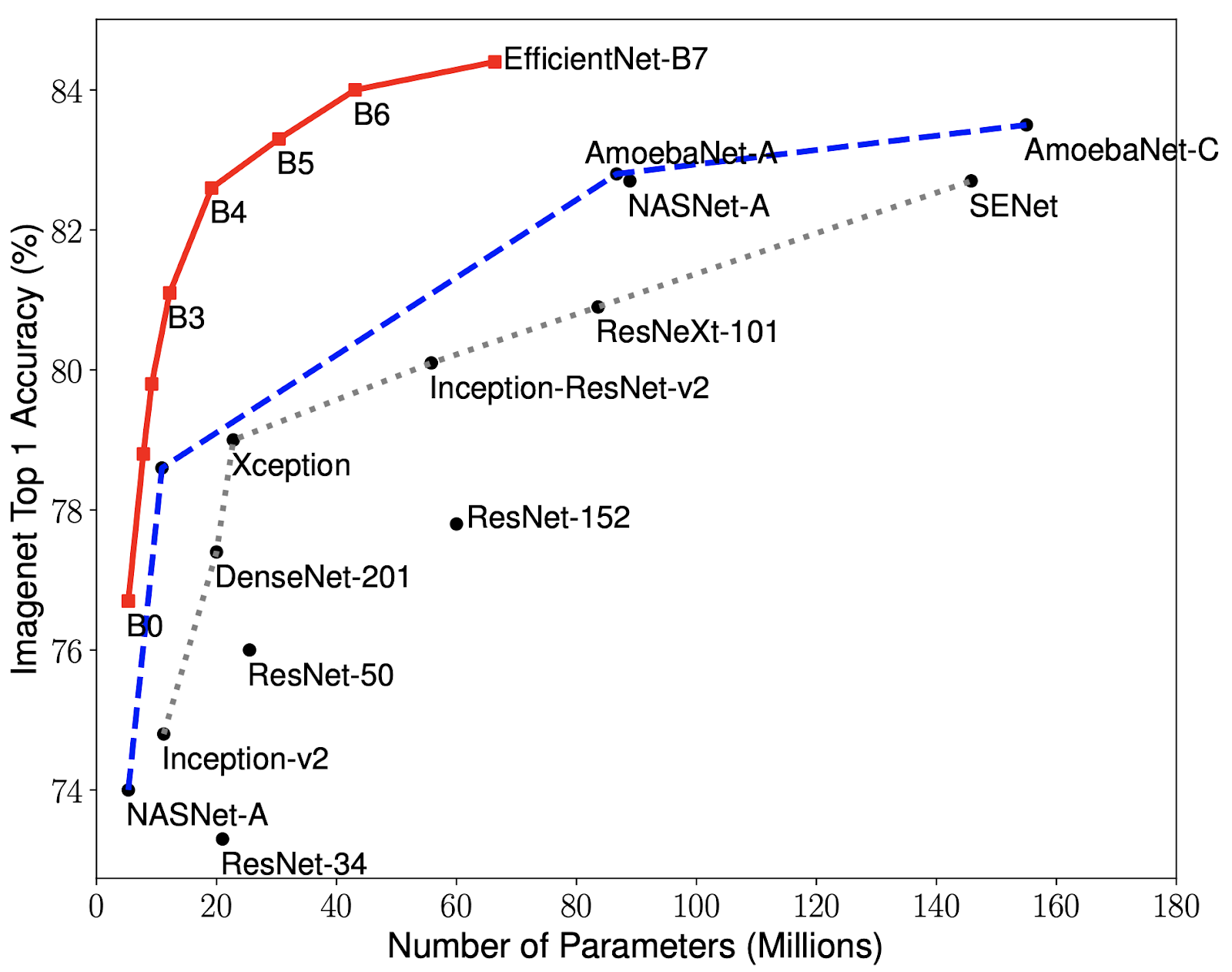 \n\n\n*Note: B7 not working due to low memory*","metadata":{}},{"cell_type":"code","source":"class EfficientNetwork(nn.Module):\n def __init__(self, output_size, no_columns, b4=False, b2=False):\n super().__init__()\n self.b4, self.b2, self.no_columns = b4, b2, no_columns\n \n # Define Feature part (IMAGE)\n if b4:\n self.features = EfficientNet.from_pretrained('efficientnet-b4')\n elif b2:\n self.features = EfficientNet.from_pretrained('efficientnet-b2')\n else:\n self.features = EfficientNet.from_pretrained('efficientnet-b7')\n \n # (CSV)\n self.csv = nn.Sequential(nn.Linear(self.no_columns, 250),\n nn.BatchNorm1d(250),\n nn.ReLU(),\n nn.Dropout(p=0.2),\n \n nn.Linear(250, 250),\n nn.BatchNorm1d(250),\n nn.ReLU(),\n nn.Dropout(p=0.2))\n \n # Define Classification part\n if b4:\n self.classification = nn.Sequential(nn.Linear(1792 + 250, output_size))\n elif b2:\n self.classification = nn.Sequential(nn.Linear(1408 + 250, output_size))\n else:\n self.classification = nn.Sequential(nn.Linear(2560 + 250, output_size))\n \n \n def forward(self, image, csv_data, prints=False): \n \n if prints: print('Input Image shape:', image.shape, '\\n'+\n 'Input csv_data shape:', csv_data.shape)\n \n # IMAGE CNN\n image = self.features.extract_features(image)\n if prints: print('Features Image shape:', image.shape)\n \n if self.b4:\n image = F.avg_pool2d(image, image.size()[2:]).reshape(-1, 1792)\n elif self.b2:\n image = F.avg_pool2d(image, image.size()[2:]).reshape(-1, 1408)\n else:\n image = F.avg_pool2d(image, image.size()[2:]).reshape(-1, 2560)\n if prints: print('Image Reshaped shape:', image.shape)\n \n # CSV FNN\n csv_data = self.csv(csv_data)\n if prints: print('CSV Data:', csv_data.shape)\n \n # Concatenate\n image_csv_data = torch.cat((image, csv_data), dim=1)\n \n # CLASSIF\n out = self.classification(image_csv_data)\n if prints: print('Out shape:', out.shape)\n \n return out","metadata":{"trusted":true},"outputs":[],"execution_count":null},{"cell_type":"markdown","source":"### How is EfficientNet working?\n\n> A schema of the below example:\n
 ","metadata":{}},{"cell_type":"code","source":"# Create an example model - Effnet\nmodel_example = EfficientNetwork(output_size=output_size, no_columns=no_columns,\n b4=False, b2=True)","metadata":{"trusted":true},"outputs":[],"execution_count":null},{"cell_type":"code","source":"# Data object and Loader\nexample_data = MelanomaDataset(train_df, vertical_flip=0.5, horizontal_flip=0.5, \n is_train=True, is_valid=False, is_test=False)\nexample_loader = torch.utils.data.DataLoader(example_data, batch_size = 3, shuffle=True)\n\n# Get a sample\nfor (image, csv_data), labels in example_loader:\n image_example, csv_data_example = image, csv_data\n labels_example = torch.tensor(labels, dtype=torch.float32)\n break\nprint('Data shape:', image_example.shape, '| \\n' , csv_data_example)\nprint('Label:', labels_example, '\\n')\n\n# Outputs\nout = model_example(image_example, csv_data_example, prints=True)\n\n# Criterion example\ncriterion_example = nn.BCEWithLogitsLoss()\n# Unsqueeze(1) from shape=[3] to shape=[3, 1]\nloss = criterion_example(out, labels_example.unsqueeze(1)) \nprint('Loss:', loss.item())","metadata":{"trusted":true},"outputs":[],"execution_count":null},{"cell_type":"markdown","source":"# 4. Training ... 💻\n\n### Prepare OOF and Predictions Matrixes\n> `OOF` will be used to assess the overall ROC value of the entire Train data (Train + Valid)","metadata":{}},{"cell_type":"code","source":"# ----- STATICS -----\ntrain_len = len(train_df)\ntest_len = len(test_df)\n# -------------------\n\n\n# Out of Fold Predictions\noof = np.zeros(shape = (train_len, 1))\n\n# Predictions\npreds_submission = torch.zeros(size = (test_len, 1), dtype=torch.float32, device=device)\n\nprint('oof shape:', oof.shape, '\\n' +\n 'predictions shape:', preds_submission.shape)","metadata":{"trusted":true},"outputs":[],"execution_count":null},{"cell_type":"markdown","source":"### GroupKFold() 🦗🦗🦗\n> K-fold iterator variant with non-overlapping groups. The same group **will not appear** in two different folds (the number of distinct groups has to be at least equal to the number of folds).\n\n> We're using `patient_id` for our grouping column: there are multiple patients with *multiple images taken*, so we need to be careful with that.\n
 ","metadata":{}},{"cell_type":"code","source":"# ----- STATICS -----\nk = 6 # number of folds in Group K Fold\n# -------------------","metadata":{"trusted":true},"outputs":[],"execution_count":null},{"cell_type":"code","source":"# Create Object\ngroup_fold = GroupKFold(n_splits = k)\n\n# Generate indices to split data into training and test set.\nfolds = group_fold.split(X = np.zeros(train_len), \n y = train_df['target'], \n groups = train_df['ID'].tolist())","metadata":{"trusted":true},"outputs":[],"execution_count":null},{"cell_type":"markdown","source":"## 4.1 Training Loop... 🔋\n\n\nBefore, I would like to thank again to Roman for the notebook Melanoma. Pytorch starter. EfficientNet. The following Training Loop is very much taken from him, but I FINALLY understood what is TTA, how to optimize the learning rate and how to use K Fold in Deep Learning. I am very happy with what I learned during this process, so I am ready to take it further and even maybe make it better?\n
Next step would be to also incorporate the data from the .csv file
\n\n\n\n* `ReduceLROnPlateau()`: Reduce learning rate when a metric has stopped improving. Here `patience` is set to 1, meaning that if 1 model doesn't improve, then the `lr` will decrease by a factor of 0.2.\n* `patience`: Early Stopping Patience (how many epochs to wait with no improvement until it stops)\n* `TTA`: Test Time Augmentation Rounds (creating multiple augmented copies of each image in the test set, having the model make a prediction for each, then returning an ensemble of those predictions)\n\n> The following chunk of code is quite big, so I made a schema of the overall steps we're taking within it:\n ","metadata":{}},{"cell_type":"code","source":"# ----- STATICS -----\nepochs = 15\npatience = 3\nTTA = 3\nnum_workers = 8\nlearning_rate = 0.0005\nweight_decay = 0.0\nlr_patience = 1 # 1 model not improving until lr is decreasing\nlr_factor = 0.4 # by how much the lr is decreasing\n\nbatch_size1 = 32\nbatch_size2 = 16\n\nversion = 'v6' # to keep tabs on versions\n# -------------------","metadata":{"trusted":true},"outputs":[],"execution_count":null},{"cell_type":"code","source":"def train_folds(preds_submission, model, version = 'v1'):\n # Creates a .txt file that will contain the logs\n f = open(f\"logs_{version}.txt\", \"w+\")\n \n \n for fold, (train_index, valid_index) in enumerate(folds):\n # Append to .txt\n with open(f\"logs_{version}.txt\", 'a+') as f:\n print('-'*10, 'Fold:', fold+1, '-'*10, file=f)\n print('-'*10, 'Fold:', fold+1, '-'*10)\n\n\n # --- Create Instances ---\n # Best ROC score in this fold\n best_roc = None\n # Reset patience before every fold\n patience_f = patience\n \n # Initiate the model\n model = model\n\n optimizer = torch.optim.Adam(model.parameters(), lr = learning_rate, weight_decay=weight_decay)\n scheduler = ReduceLROnPlateau(optimizer=optimizer, mode='max', \n patience=lr_patience, verbose=True, factor=lr_factor)\n criterion = nn.BCEWithLogitsLoss()\n\n\n # --- Read in Data ---\n train_data = train_df.iloc[train_index].reset_index(drop=True)\n valid_data = train_df.iloc[valid_index].reset_index(drop=True)\n\n # Create Data instances\n train = MelanomaDataset(train_data, vertical_flip=vertical_flip, horizontal_flip=horizontal_flip, \n is_train=True, is_valid=False, is_test=False)\n valid = MelanomaDataset(valid_data, vertical_flip=vertical_flip, horizontal_flip=horizontal_flip, \n is_train=False, is_valid=True, is_test=False)\n # Read in test data | Remember! We're using data augmentation like we use for Train data.\n test = MelanomaDataset(test_df, vertical_flip=vertical_flip, horizontal_flip=horizontal_flip,\n is_train=False, is_valid=False, is_test=True)\n\n # Dataloaders\n train_loader = DataLoader(train, batch_size=batch_size1, shuffle=True, num_workers=num_workers)\n # shuffle=False! Otherwise function won't work!!!\n # how do I know? ^^\n valid_loader = DataLoader(valid, batch_size=batch_size2, shuffle=False, num_workers=num_workers)\n test_loader = DataLoader(test, batch_size=batch_size2, shuffle=False, num_workers=num_workers)\n\n\n # === EPOCHS ===\n for epoch in range(epochs):\n start_time = time.time()\n correct = 0\n train_losses = 0\n\n # === TRAIN ===\n # Sets the module in training mode.\n model.train()\n\n for (images, csv_data), labels in train_loader:\n # Save them to device\n images = torch.tensor(images, device=device, dtype=torch.float32)\n csv_data = torch.tensor(csv_data, device=device, dtype=torch.float32)\n labels = torch.tensor(labels, device=device, dtype=torch.float32)\n\n # Clear gradients first; very important, usually done BEFORE prediction\n optimizer.zero_grad()\n\n # Log Probabilities & Backpropagation\n out = model(images, csv_data)\n loss = criterion(out, labels.unsqueeze(1))\n loss.backward()\n optimizer.step()\n\n # --- Save information after this batch ---\n # Save loss\n train_losses += loss.item()\n # From log probabilities to actual probabilities\n train_preds = torch.round(torch.sigmoid(out)) # 0 and 1\n # Number of correct predictions\n correct += (train_preds.cpu() == labels.cpu().unsqueeze(1)).sum().item()\n\n # Compute Train Accuracy\n train_acc = correct / len(train_index)\n\n\n # === EVAL ===\n # Sets the model in evaluation mode\n model.eval()\n\n # Create matrix to store evaluation predictions (for accuracy)\n valid_preds = torch.zeros(size = (len(valid_index), 1), device=device, dtype=torch.float32)\n\n\n # Disables gradients (we need to be sure no optimization happens)\n with torch.no_grad():\n for k, ((images, csv_data), labels) in enumerate(valid_loader):\n images = torch.tensor(images, device=device, dtype=torch.float32)\n csv_data = torch.tensor(csv_data, device=device, dtype=torch.float32)\n labels = torch.tensor(labels, device=device, dtype=torch.float32)\n\n out = model(images, csv_data)\n pred = torch.sigmoid(out)\n valid_preds[k*images.shape[0] : k*images.shape[0] + images.shape[0]] = pred\n\n # Compute accuracy\n valid_acc = accuracy_score(valid_data['target'].values, \n torch.round(valid_preds.cpu()))\n # Compute ROC\n valid_roc = roc_auc_score(valid_data['target'].values, \n valid_preds.cpu())\n\n # Compute time on Train + Eval\n duration = str(datetime.timedelta(seconds=time.time() - start_time))[:7]\n\n\n # PRINT INFO\n # Append to .txt file\n with open(f\"logs_{version}.txt\", 'a+') as f:\n print('{} | Epoch: {}/{} | Loss: {:.4} | Train Acc: {:.3} | Valid Acc: {:.3} | ROC: {:.3}'.\\\n format(duration, epoch+1, epochs, train_losses, train_acc, valid_acc, valid_roc), file=f)\n # Print to console\n print('{} | Epoch: {}/{} | Loss: {:.4} | Train Acc: {:.3} | Valid Acc: {:.3} | ROC: {:.3}'.\\\n format(duration, epoch+1, epochs, train_losses, train_acc, valid_acc, valid_roc))\n\n\n # === SAVE MODEL ===\n\n # Update scheduler (for learning_rate)\n scheduler.step(valid_roc)\n\n # Update best_roc\n if not best_roc: # If best_roc = None\n best_roc = valid_roc\n torch.save(model.state_dict(),\n f\"Fold{fold+1}_Epoch{epoch+1}_ValidAcc_{valid_acc:.3f}_ROC_{valid_roc:.3f}.pth\")\n continue\n\n if valid_roc > best_roc:\n best_roc = valid_roc\n # Reset patience (because we have improvement)\n patience_f = patience\n torch.save(model.state_dict(),\n f\"Fold{fold+1}_Epoch{epoch+1}_ValidAcc_{valid_acc:.3f}_ROC_{valid_roc:.3f}.pth\")\n else:\n # Decrease patience (no improvement in ROC)\n patience_f = patience_f - 1\n if patience_f == 0:\n with open(f\"logs_{version}.txt\", 'a+') as f:\n print('Early stopping (no improvement since 3 models) | Best ROC: {}'.\\\n format(best_roc), file=f)\n print('Early stopping (no improvement since 3 models) | Best ROC: {}'.\\\n format(best_roc))\n break\n\n\n # === INFERENCE ===\n # Choose model with best_roc in this fold\n best_model_path = '../working/' + [file for file in os.listdir('../working') if str(round(best_roc, 3)) in file and 'Fold'+str(fold+1) in file][0]\n # Using best model from Epoch Train\n # !!!!!!!!!!!!!!!!!!!!!!!!!!!!!!!!!\n model = EfficientNetwork(output_size = output_size, no_columns=no_columns,\n b4=False, b2=True).to(device)\n model.load_state_dict(torch.load(best_model_path))\n # Set the model in evaluation mode\n model.eval()\n\n\n with torch.no_grad():\n # --- EVAL ---\n # Predicting again on Validation data to get preds for OOF\n valid_preds = torch.zeros(size = (len(valid_index), 1), device=device, dtype=torch.float32)\n\n for k, ((images, csv_data), _) in enumerate(valid_loader):\n images = torch.tensor(images, device=device, dtype=torch.float32)\n csv_data = torch.tensor(csv_data, device=device, dtype=torch.float32)\n\n out = model(images, csv_data)\n pred = torch.sigmoid(out)\n valid_preds[k*images.shape[0] : k*images.shape[0] + images.shape[0]] = pred\n\n # Save info to OOF\n oof[valid_index] = valid_preds.cpu().numpy()\n\n\n # --- TEST ---\n # Now (Finally) prediction for our TEST data\n for i in range(TTA):\n for k, (images, csv_data) in enumerate(test_loader):\n images = torch.tensor(images, device=device, dtype=torch.float32)\n csv_data = torch.tensor(csv_data, device=device, dtype=torch.float32)\n\n out = model(images, csv_data)\n # Covert to probablities\n out = torch.sigmoid(out)\n\n # ADDS! the prediction to the matrix we already created\n preds_submission[k*images.shape[0] : k*images.shape[0] + images.shape[0]] += out\n\n\n # Divide Predictions by TTA (to average the results during TTA)\n preds_submission /= TTA\n\n\n # === CLEANING ===\n # Clear memory\n del train, valid, train_loader, valid_loader, images, labels\n # Garbage collector\n gc.collect()","metadata":{"trusted":true},"outputs":[],"execution_count":null},{"cell_type":"markdown","source":"### #Training in progress... 🛫 Please do not disturb","metadata":{}},{"cell_type":"code","source":"!pip install polars","metadata":{"trusted":true},"outputs":[],"execution_count":null},{"cell_type":"code","source":"import os\nimport itertools\nfrom pathlib import Path\n\nimport numpy as np\nimport pandas as pd\nimport polars as pl\n\nfrom sklearn.model_selection import StratifiedGroupKFold\nfrom sklearn.model_selection import cross_val_score\nfrom sklearn.preprocessing import OneHotEncoder\nfrom sklearn.metrics import roc_auc_score\nfrom sklearn.ensemble import VotingClassifier\n\nfrom imblearn.under_sampling import RandomUnderSampler\nfrom imblearn.pipeline import Pipeline\n\nimport lightgbm as lgb\n\nimport warnings\nwarnings.filterwarnings(\"ignore\")","metadata":{"trusted":true},"outputs":[],"execution_count":null},{"cell_type":"code","source":"","metadata":{},"outputs":[],"execution_count":null}]}
#1: Different skin tones. Might need to find something that levels that.
\n#2: Different lightings in the image.
\n#3: Different sizes of the images. We need to resize them.
\nNext step would be to also incorporate the data from the .csv file
\n