{"cells":[{"metadata":{"_uuid":"44286973-5d23-45f3-9e27-aa5f13d73951","_cell_guid":"baac03d8-7e5e-46a6-b92e-910c3ac63029","trusted":true},"cell_type":"markdown","source":"**In this kernel we will like to analyze images and  if possible (measure size of spots) and also some  data augmentation ideas that looks promising**","execution_count":null},{"metadata":{"_uuid":"3597d34f-11f1-48f3-b59d-14281f14c930","_cell_guid":"e9e7676b-af53-40da-a5f6-94d6c794b6ce","trusted":true},"cell_type":"markdown","source":"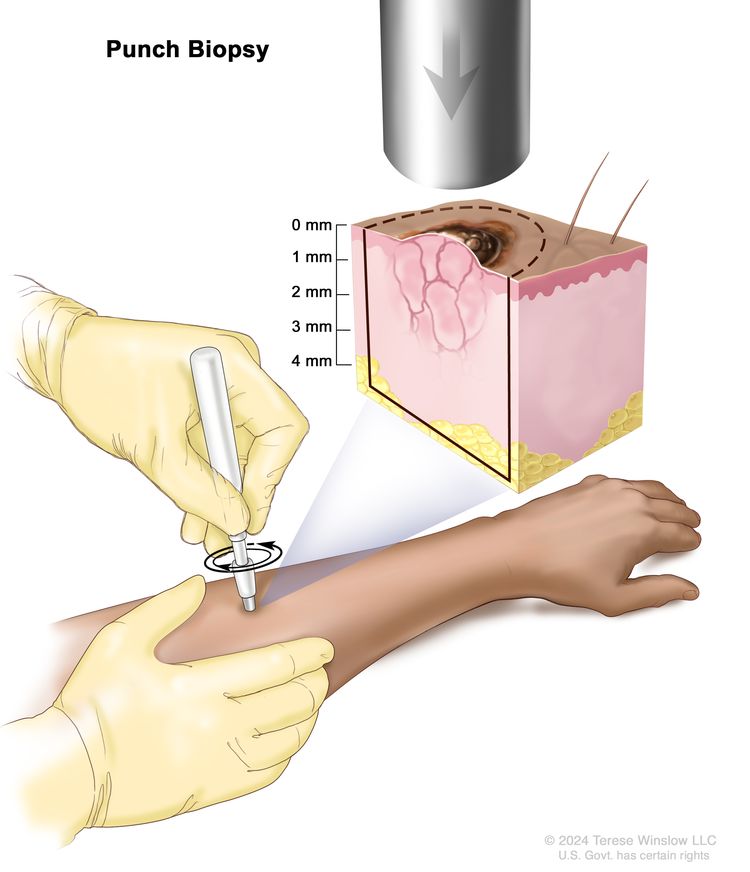![](https://nci-media.cancer.gov/pdq/media/images/578083-750.jpg)","execution_count":null},{"metadata":{"_uuid":"99143a69-3c76-4315-9fa5-8153bcbb1063","_cell_guid":"290bbefd-b496-4af2-98a5-f072f8dc3f59","trusted":true},"cell_type":"markdown","source":"if you are a researcher, then probably you will like to spend some times analyzing melanoma mole sizes as i have shown LEVELS OF MELANOMA in my past kernel [In-Depth Melanoma with modeling](https://www.kaggle.com/mobassir/in-depth-melanoma-with-modeling) so we know that.... <br> <br> **The Clark Scale has 5 levels of melanoma:**\n\n* Cells are in the out layer of the skin (epidermis)\n\n* Cells are in the layer directly under the epidermis (pupillary dermis)\n\n* The cells are touching the next layer known as the deep dermis\n\n* Cells have spread to the reticular dermis\n\n* Cells have grown in the fat layer\n\n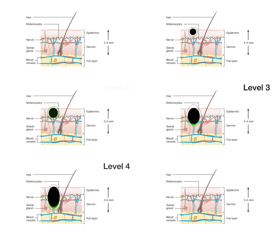![](https://media.giphy.com/media/lSJElktZ5BKUvYSztq/giphy.gif)","execution_count":null},{"metadata":{"_uuid":"a6e37fcb-bb1b-4907-8b1d-2a588e54aed6","_cell_guid":"f6b16312-3ce1-413c-8840-6ec06a353251","trusted":true},"cell_type":"markdown","source":"# References","execution_count":null},{"metadata":{"_uuid":"a31c1940-7e19-4f6e-817b-cc62b9be5acc","_cell_guid":"c9be6717-6b18-4dad-ab8f-ea0cee043cac","trusted":true},"cell_type":"markdown","source":"* [TensorFlow + Transfer Learning: Melanoma](https://www.kaggle.com/amyjang/tensorflow-transfer-learning-melanoma)\n* [Measuring size of objects in an image with OpenCV](https://www.pyimagesearch.com/2016/03/28/measuring-size-of-objects-in-an-image-with-opencv/)\n* [object-size](https://github.com/snsharma1311/object-size)\n* [Ensemble of Convolutional Neural Networks for Disease Classification of Skin Lesions](https://github.com/anindox8/Ensemble-of-Multi-Scale-CNN-for-Dermatoscopy-Classification)\n* [In-Depth Melanoma with modeling](https://www.kaggle.com/mobassir/in-depth-melanoma-with-modeling?scriptVersionId=39094350)\n* [GENERAL INFORMATION ABOUT MELANOMA](https://www.uhhospitals.org/services/cancer-services/skin-cancer/melanoma/about-melanoma)\n\n* [[Training CV] Melanoma Starter](https://www.kaggle.com/shonenkov/training-cv-melanoma-starter)\n\n* [Measuring Size of Objects with OpenCV](https://github.com/Practical-CV/Measuring-Size-of-Objects-with-OpenCV)\n* [Color Constancy](https://github.com/MinaSGorgi/Color-Constancy)\n* [Edge-Based Color Constancy](https://ieeexplore.ieee.org/document/4287009)\n* [Python | Thresholding techniques using OpenCV | Set-1 (Simple Thresholding)](https://www.geeksforgeeks.org/python-thresholding-techniques-using-opencv-set-1-simple-thresholding/)\n* [lesion-GAN](https://github.com/alxiang/lesion-GAN)\n* [Data-Augmentation-and-Segmentation-with-GANs-for-Medical-Images](https://github.com/apolanco3225/Data-Augmentation-and-Segmentation-with-GANs-for-Medical-Images)\n* [Towards Interpretable Skin Lesion Classification with Deep Learning Models](https://www.ncbi.nlm.nih.gov/pmc/articles/PMC7153112/pdf/3203149.pdf)","execution_count":null},{"metadata":{"_uuid":"89ece5d6-81d1-4b6d-860e-5fe6bfb8100c","_cell_guid":"18f9598c-befd-420b-9eb2-8a52edab99b1","trusted":true},"cell_type":"markdown","source":"# imports","execution_count":null},{"metadata":{"_uuid":"e4d43621-7637-4e1a-ac7d-3c474c16dc5d","_cell_guid":"78060f4a-d066-4420-8fda-3264f446cb33","trusted":true,"_kg_hide-input":true,"_kg_hide-output":true},"cell_type":"code","source":"!pip install imutils","execution_count":null,"outputs":[]},{"metadata":{"_uuid":"db06302c-65f8-4a89-8f59-1786e2c81058","_cell_guid":"9db37ec0-c5d9-4923-bdfe-6cddff45cb3e","trusted":true,"_kg_hide-input":true,"_kg_hide-output":true},"cell_type":"code","source":"# This Python 3 environment comes with many helpful analytics libraries installed\n# It is defined by the kaggle/python Docker image: https://github.com/kaggle/docker-python\n# For example, here's several helpful packages to load\nfrom __future__ import unicode_literals\nfrom __future__ import print_function\nfrom __future__ import division\nfrom __future__ import absolute_import\nimport numpy as np # linear algebra\nimport pandas as pd # data processing, CSV file I/O (e.g. pd.read_csv)\n\n# Input data files are available in the read-only \"../input/\" directory\n# For example, running this (by clicking run or pressing Shift+Enter) will list all files under the input directory\nfrom pathlib import Path\nimport pandas as pd\nfrom torch.utils.data import Dataset,DataLoader\n\nfrom scipy.spatial import distance as dist\nfrom imutils import perspective\nfrom imutils import contours\nimport matplotlib.pyplot as plt\nimport numpy as np\nimport imutils\nimport cv2\n\nimport skimage.measure\nimport imageio\nfrom PIL import Image\nimport requests\nfrom io import BytesIO\nfrom torchvision import transforms as T\nimport torch.nn as nn\nimport torch\nimport torch.nn.functional as F\nfrom sklearn.model_selection import GroupKFold\nfrom kaggle_datasets import KaggleDatasets\n\nfrom scipy.spatial.distance import euclidean\nfrom imutils import perspective\nfrom imutils import contours\nimport numpy as np\nimport imutils\nimport cv2\nimport matplotlib.pyplot as plt\n\nfrom glob import glob\nimport pandas as pd\nfrom sklearn.model_selection import GroupKFold\nimport cv2\nfrom skimage import io\nimport albumentations as A\nimport torch\nimport os\nfrom datetime import datetime\nimport time\nimport random\nimport cv2\nimport pandas as pd\nimport numpy as np\nimport albumentations as A\nimport matplotlib.pyplot as plt\nfrom albumentations.pytorch.transforms import ToTensorV2\nfrom sklearn.model_selection import StratifiedKFold\nfrom torch.utils.data import Dataset,DataLoader\nfrom torch.utils.data.sampler import SequentialSampler, RandomSampler\nfrom torch.nn import functional as F\nfrom glob import glob\nimport sklearn\nfrom torch import nn\n\n\nimport keras\nimport numpy as np\nimport tensorflow as tf\nfrom keras.models import model_from_json, load_model\nimport json\n\nimport matplotlib.pyplot as plt\n\nfrom sklearn.model_selection import train_test_split\nimport tensorflow as tf\nfrom functools import partial\n\nimport glob\nimport numpy as np\nimport cv2\nfrom skimage import filters as skifilters\nfrom scipy import ndimage\nfrom skimage import filters\nimport matplotlib.pyplot as plt\nimport tqdm\nfrom sklearn.utils import shuffle\nimport pandas as pd\n\nimport os\nimport h5py\nimport time\nimport json\nimport warnings\nfrom PIL import Image\n\nfrom fastprogress.fastprogress import master_bar, progress_bar\nfrom sklearn.metrics import accuracy_score, roc_auc_score\nfrom torchvision import models\nimport pdb\nimport albumentations as A\nfrom albumentations.pytorch.transforms import ToTensor\nimport matplotlib.pyplot as plt\n\nimport pickle \nimport os\n\n# You can write up to 5GB to the current directory (/kaggle/working/) that gets preserved as output when you create a version using \"Save & Run All\" \n# You can also write temporary files to /kaggle/temp/, but they won't be saved outside of the current session","execution_count":null,"outputs":[]},{"metadata":{"_uuid":"080ff8b4-3e85-47b7-8305-d7c2876612eb","_cell_guid":"17714261-aaa4-4af2-bd57-90966fb942c3","trusted":true},"cell_type":"code","source":"def list_files(path:Path):\n    return [o for o in path.iterdir()]","execution_count":null,"outputs":[]},{"metadata":{"_uuid":"64314ff8-eb28-4f0a-aa2a-64cacf51ce66","_cell_guid":"a3f5a768-1b34-48fb-b8dd-fa56b7edf476","trusted":true},"cell_type":"code","source":"path = Path('../input/jpeg-melanoma-768x768/')\ndf_path = Path('../input/jpeg-melanoma-768x768/')\nim_sz = 256\nbs = 16","execution_count":null,"outputs":[]},{"metadata":{"_uuid":"d079867c-a374-410d-bb39-982cae170334","_cell_guid":"17841ecb-653e-44e8-af3d-53e7fb2e9504","trusted":true},"cell_type":"code","source":"train_fnames = list_files(path/'train')\ndf = pd.read_csv(df_path/'train.csv')\ndf.head()","execution_count":null,"outputs":[]},{"metadata":{"_uuid":"d4ec5043-b959-43b0-8da3-228da4931942","_cell_guid":"9a9f78c8-f790-48eb-865a-f9f0e29754da","trusted":true},"cell_type":"code","source":"\n\ndf.target.value_counts(),df.shape","execution_count":null,"outputs":[]},{"metadata":{"_uuid":"17eb57a2-357e-4803-9bea-3f6e36dce0e2","_cell_guid":"5ee150ab-7da8-4f09-a315-b98fd4dbdf6d","trusted":true},"cell_type":"code","source":"\nGCS_PATH = KaggleDatasets().get_gcs_path('melanoma-768x768')","execution_count":null,"outputs":[]},{"metadata":{"_uuid":"722e8d6b-68d3-44ed-97f6-250cafd01802","_cell_guid":"5c676e58-9982-442e-adcb-8da0c89addda","trusted":true},"cell_type":"code","source":"def decode_image(image):\n    image = tf.image.decode_jpeg(image, channels=3)\n    image = tf.cast(image, tf.float32) / 255.0\n    image = tf.reshape(image, [*IMAGE_SIZE, 3])\n    return image","execution_count":null,"outputs":[]},{"metadata":{"_uuid":"5f29a4e5-c8fa-4423-8b6a-e885edab0969","_cell_guid":"cc796e6c-8b5e-446a-b1a7-8ae055f50b4f","trusted":true},"cell_type":"code","source":"def read_tfrecord(example, labeled):\n    tfrecord_format = {\n        \"image\": tf.io.FixedLenFeature([], tf.string),\n        \"target\": tf.io.FixedLenFeature([], tf.int64)\n    } if labeled else {\n        \"image\": tf.io.FixedLenFeature([], tf.string),\n        \"image_name\": tf.io.FixedLenFeature([], tf.string)\n    }\n    example = tf.io.parse_single_example(example, tfrecord_format)\n    image = decode_image(example['image'])\n    if labeled:\n        label = tf.cast(example['target'], tf.int32)\n        return image, label\n    idnum = example['image_name']\n    return image, idnum","execution_count":null,"outputs":[]},{"metadata":{"_uuid":"7cb62ebd-3ff4-4828-8565-dfdeaff21cc1","_cell_guid":"e4dbb3bb-04d7-4862-8cd3-56e424338a4f","trusted":true},"cell_type":"code","source":"def load_dataset(filenames, labeled=True, ordered=False):\n    ignore_order = tf.data.Options()\n    if not ordered:\n        ignore_order.experimental_deterministic = False # disable order, increase speed\n    dataset = tf.data.TFRecordDataset(filenames, num_parallel_reads=AUTOTUNE) # automatically interleaves reads from multiple files\n    dataset = dataset.with_options(ignore_order) # uses data as soon as it streams in, rather than in its original order\n    dataset = dataset.map(partial(read_tfrecord, labeled=labeled), num_parallel_calls=AUTOTUNE)\n    # returns a dataset of (image, label) pairs if labeled=True or (image, id) pairs if labeled=False\n    return dataset","execution_count":null,"outputs":[]},{"metadata":{"_uuid":"86127897-7a05-4772-9a8c-8abf32fa082e","_cell_guid":"470445ab-c42c-465d-bce7-1376d103fb5d","trusted":true},"cell_type":"code","source":"\nBATCH_SIZE = 8\nAUTOTUNE = tf.data.experimental.AUTOTUNE\nIMAGE_SIZE = [768, 768]\nTRAINING_FILENAMES, VALID_FILENAMES = train_test_split(\n    tf.io.gfile.glob(GCS_PATH + '/train*.tfrec'),\n    test_size=0.2, random_state=5\n)\nTEST_FILENAMES = tf.io.gfile.glob(GCS_PATH + '/test*.tfrec')\nprint('Train TFRecord Files:', len(TRAINING_FILENAMES))\nprint('Validation TFRecord Files:', len(VALID_FILENAMES))\nprint('Test TFRecord Files:', len(TEST_FILENAMES))","execution_count":null,"outputs":[]},{"metadata":{"_uuid":"61fd6ecd-627a-4f18-964f-b04c7da67bae","_cell_guid":"9ce64f61-e490-46fc-b565-14366a74403b","trusted":true},"cell_type":"code","source":"\n\ndef get_training_dataset():\n    dataset = load_dataset(TRAINING_FILENAMES, labeled=True)\n    #dataset = dataset.map(augmentation_pipeline, num_parallel_calls=AUTOTUNE)\n    dataset = dataset.repeat()\n    dataset = dataset.shuffle(2048)\n    dataset = dataset.batch(BATCH_SIZE)\n    dataset = dataset.prefetch(AUTOTUNE)\n    return dataset","execution_count":null,"outputs":[]},{"metadata":{"_uuid":"a9827661-2782-4212-8f4a-de5dba6cffb8","_cell_guid":"60702fda-834e-4bd1-bf8e-8055fcf2ec8b","trusted":true},"cell_type":"code","source":"train_dataset = get_training_dataset()","execution_count":null,"outputs":[]},{"metadata":{"_uuid":"0f2df332-35a3-4cfb-a020-a71658adf22d","_cell_guid":"47c9466b-50d8-4512-9119-9e57cc6b7be2","trusted":true},"cell_type":"code","source":"def show_batch(image_batch, label_batch):\n    plt.figure(figsize=(15,15))\n    for n in range(8):\n        ax = plt.subplot(8,8,n+1)\n        plt.imshow(image_batch[n])\n        if label_batch[n]:\n            plt.title(\"MALIGNANT(1)\")\n        else:\n            plt.title(\"BENIGN(0)\")\n        plt.axis(\"off\")","execution_count":null,"outputs":[]},{"metadata":{"_uuid":"b4f09a90-ef5a-481f-bd81-e3b44be95f8b","_cell_guid":"4fd271fe-fccf-4db3-8046-a5d2f3d2161d","trusted":true},"cell_type":"code","source":"%%time\nfor i in range(0,10):\n    image_batch, label_batch = next(iter(train_dataset))\n    for j in range(0,8):\n        var = label_batch[j].numpy()\n        if(var!=0):\n            show_batch(image_batch.numpy(), label_batch.numpy())","execution_count":null,"outputs":[]},{"metadata":{"_uuid":"c688e803-0393-4163-952b-00b4d9b910e6","_cell_guid":"5537ecd1-5c41-4aeb-a72c-160cb40bed9c","trusted":true},"cell_type":"code","source":"print(\"Samples with Melanoma\")\nimgs = df[df.target==1]['image_name'].values\n_, axs = plt.subplots(2, 3, figsize=(20, 8))\naxs = axs.flatten()\nfor f_name,ax in zip(imgs[10:20],axs):\n    img = Image.open(path/f'train/{f_name}.jpg')\n    ax.imshow(img)\n    ax.axis('off')    \nplt.show()","execution_count":null,"outputs":[]},{"metadata":{"_uuid":"a736cf02-c0f5-4c79-b3bf-08ab409a6b1c","_cell_guid":"7d02d7f2-99a4-4508-9b65-60d4fd56e775","trusted":true},"cell_type":"markdown","source":"The thickness of the tumor. The thickness of the tumor is measured from the surface of the skin to the deepest part of the tumor.\n\n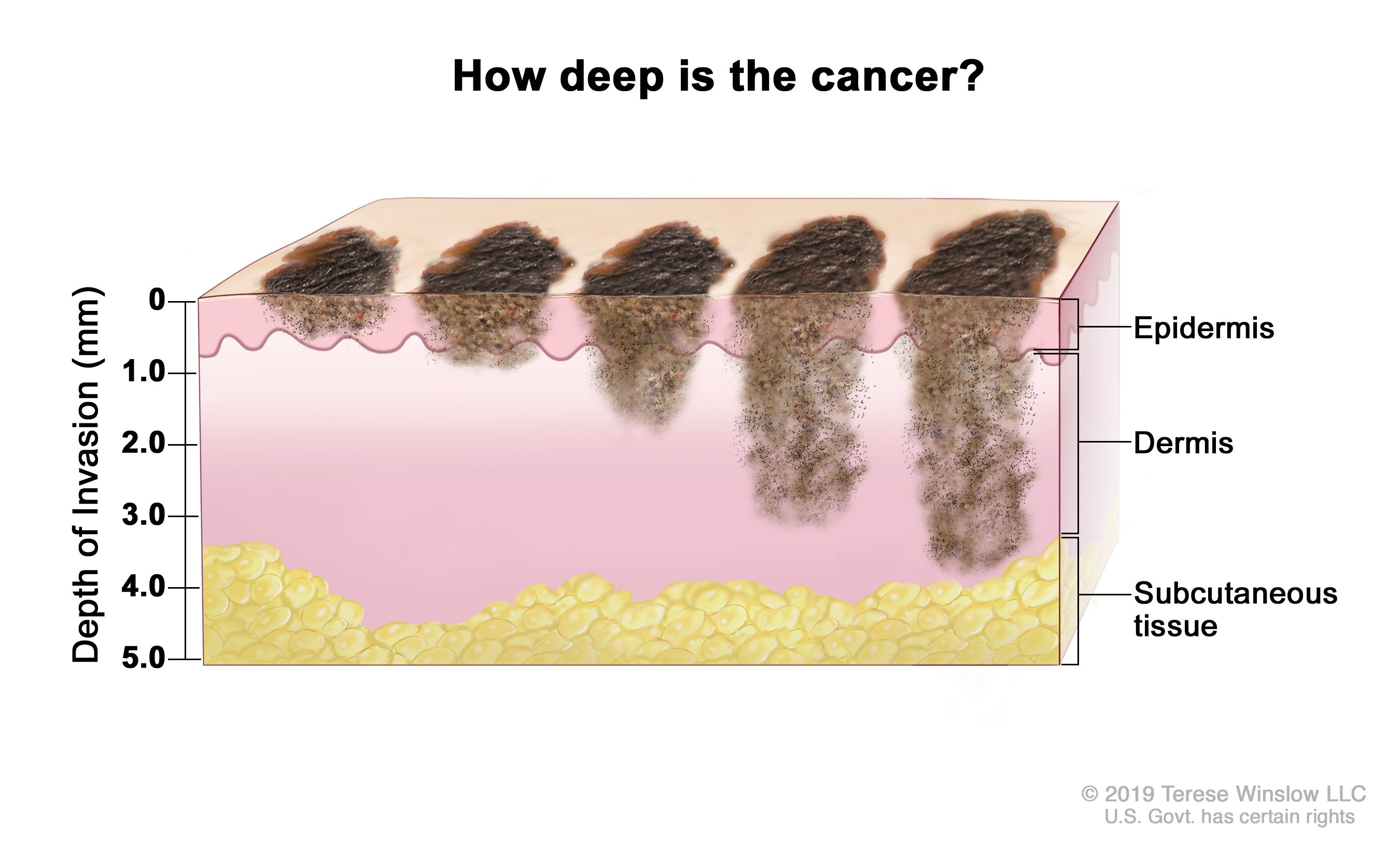![](https://nci-media.cancer.gov/pdq/media/images/799465.jpg)","execution_count":null},{"metadata":{"_uuid":"bb81269d-3d43-4577-953f-c9da93a65989","_cell_guid":"a89d6bd2-065b-4f97-884d-b5fb735d797e","trusted":true},"cell_type":"markdown","source":"**Whether the tumor is ulcerated (has broken through the skin).**\n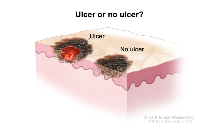![](https://nci-media.cancer.gov/pdq/media/images/799466-750.jpg)","execution_count":null},{"metadata":{"_uuid":"7726e086-5c32-4ebd-856c-056822677fe9","_cell_guid":"5735f895-b36a-4e44-bc4c-b1e9df853a72","trusted":true},"cell_type":"markdown","source":"from above 2 images we can see that depth of melanoma increases  as the mole size grows","execution_count":null},{"metadata":{"_uuid":"34d5a811-671d-4f43-b962-2702141bd3d3","_cell_guid":"60c68c6e-953d-4ed4-8d7c-a129b702ae24","trusted":true},"cell_type":"markdown","source":"# Algorithm","execution_count":null},{"metadata":{"_uuid":"123d8a1d-98eb-42e3-8da4-f096cb5d2fba","_cell_guid":"2a181090-f4b1-4698-8757-850adda3eb8f","trusted":true},"cell_type":"markdown","source":"1. Image pre-processing\n - Read an image and convert it it no grayscale\n - Blur the image using Gaussian Kernel to remove un-necessary edges\n - Edge detection using Canny edge detector\n - Perform morphological closing operation to remove noisy contours\n2. Object Segmentation\n - Find contours\n - Remove small contours by calculating its area (threshold used here is 100)\n - Sort contours from left to right to find the reference objects\n3. Reference object\n - Calculate how many pixels are there per metric (centi meter is used here)\n4. Compute results\n - Draw bounding boxes around each object and calculate its height and width","execution_count":null},{"metadata":{"_uuid":"2e5b8e5c-21ab-44b0-91dc-43e3c778df46","_cell_guid":"68ebbc2e-7ca8-4cc8-a051-632c826d47dd","trusted":true},"cell_type":"code","source":"\n# Usage: This script will measure different objects in the frame using a reference object \n\n\n\n# Function to show array of images (intermediate results)\n\ndef show_images(images):\n    for i, img in enumerate(images):\n        plt.figure(figsize=(20,20))\n        plt.imshow(img)\n        plt.show()\n       \n\n        \nimgs = df[df.target==1]['image_name'].values\nprint(\"Samples with Melanoma\")\nfor f_name,ax in zip(imgs[:100],axs):\n \n    \n    im1 = Image.open(path/f'train/{f_name}.jpg')\n    print(path/f'train/{f_name}.jpg')\n    im1.save('./a.png')\n    img_path = '../working/a.png'\n\n\n\n    '''load our image from disk, convert it to grayscale, and then smooth it using a Gaussian filter.\n    We then perform edge detection along with a dilation + erosion to close any gaps \n    in between edges in the edge map\n    '''\n\n    # Read image and preprocess\n    image = cv2.imread(img_path)\n \n    #image = img\n\n    gray = cv2.cvtColor(image, cv2.COLOR_BGR2GRAY)\n    blur = cv2.GaussianBlur(gray, (7, 7), 0)\n\n    edged = cv2.Canny(blur, 50, 100)\n    edged = cv2.dilate(edged, None, iterations=1)\n    edged = cv2.erode(edged, None, iterations=1)\n\n    #show_images([blur, edged])\n\n    '''find contours (i.e., the outlines) that correspond to the objects in our edge map.'''\n    # Find contours\n    cnts = cv2.findContours(edged.copy(), cv2.RETR_EXTERNAL, cv2.CHAIN_APPROX_SIMPLE)\n    cnts = imutils.grab_contours(cnts)\n\n    # Sort contours from left to right as leftmost contour is reference object\n    try:\n        '''These contours are then sorted from left-to-right (allowing us to extract our reference object)'''\n        (cnts, _) = contours.sort_contours(cnts)\n         # Remove contours which are not large enough\n        for k in range(0,20):\n            try:\n                cnts = [x for x in cnts if cv2.contourArea(x) > k]\n                # Reference object dimensions\n                # Here for reference I have used a 2cm x 2cm square\n                mid = len(cnts)//2\n                ref_object = cnts[mid]\n            except:\n                pass\n    except:\n        #print(\"An exception occurred\") \n        continue\n\n    #print(len(cnts))\n    #print(cnts)\n    #cv2.drawContours(image, cnts, -1, (0,255,0), 3)\n\n    #show_images([image, edged])\n    #print(len(cnts))\n\n    # compute the rotated bounding box of the contour\n    orig = image.copy()\n    box = cv2.minAreaRect(ref_object)\n    box = cv2.boxPoints(box)\n    box = np.array(box, dtype=\"int\")\n    \n    # order the points in the contour such that they appear\n    # in top-left, top-right, bottom-right, and bottom-left\n    # order, then draw the outline of the rotated bounding\n    # box\n    \n    box = perspective.order_points(box)\n    \n    cv2.drawContours(orig, [box.astype(\"int\")], -1, (0, 255, 0), 2)\n    # loop over the original points and draw them\n    for (x, y) in box:\n        cv2.circle(orig, (int(x), int(y)), 5, (0, 0, 255), -1)\n        \n    (tl, tr, br, bl) = box\n    dist_in_pixel = euclidean(tl, tr)\n    dist_in_cm = 2\n    pixel_per_cm = dist_in_pixel/dist_in_cm\n    largestht = []\n    largestwid = []\n    # Draw remaining contours\n    for cnt in cnts:\n        box = cv2.minAreaRect(cnt)\n        box = cv2.boxPoints(box)\n        box = np.array(box, dtype=\"int\")\n        box = perspective.order_points(box)\n        (tl, tr, br, bl) = box\n        cv2.drawContours(image, [box.astype(\"int\")], -1, (0, 0, 255), 2)\n        mid_pt_horizontal = (tl[0] + int(abs(tr[0] - tl[0])/2), tl[1] + int(abs(tr[1] - tl[1])/2))\n        mid_pt_verticle = (tr[0] + int(abs(tr[0] - br[0])/2), tr[1] + int(abs(tr[1] - br[1])/2))\n        wid = euclidean(tl, tr)/pixel_per_cm\n        ht = euclidean(tr, br)/pixel_per_cm\n        largestht.append(ht)\n        largestwid.append(wid)\n       \n        #cv2.putText(image, \"{:.1f}cm\".format(wid), (int(mid_pt_horizontal[0] - 15), int(mid_pt_horizontal[1] - 10)), \n        #cv2.FONT_HERSHEY_SIMPLEX, 0.5, (255, 255, 0), 2)\n        #cv2.putText(image, \"{:.1f}cm\".format(ht), (int(mid_pt_verticle[0] + 10), int(mid_pt_verticle[1])), \n        #cv2.FONT_HERSHEY_SIMPLEX, 0.5, (255, 255, 0), 2)\n    show_images([image])   \n    if(len(largestht)>0):\n        a = largestht.index(max(largestht))\n        b = largestwid.index(max(largestwid))\n        largestht1 = largestht[b]\n        largestwid1 = largestwid[b]\n        largestht = largestht[a]\n        largestwid = largestwid[a]\n        \n\n        print(\"Rectangle 1  has : HEIGHT = \",largestht,\"and WIDTH = \",largestwid)\n        print(\"Rectangle 2  has : HEIGHT = \",largestht1,\"and WIDTH = \",largestwid1)","execution_count":null,"outputs":[]},{"metadata":{"_uuid":"b50ac811-f3ba-498e-b0c3-0e7e349f0cb3","_cell_guid":"50f104ed-c48f-436f-a1e5-40dd38367698","trusted":true},"cell_type":"markdown","source":"from the outputs we can see that some images has scale measurements and our  object detector detected those and we can measure that scale too,but my  questions to researchers out there? - \"can we use those for any further analysis? and isn't it possible that learning algorithms focusing on such noises instead of melanoma moles?\"","execution_count":null},{"metadata":{"_uuid":"322400db-18b2-4ac3-9b9a-68fe9b6eaf53","_cell_guid":"b6cb3e74-eab8-4c0e-a4e0-c324337bf8e8","trusted":true},"cell_type":"markdown","source":"![](https://i.ibb.co/C8GkNQn/findings.png)","execution_count":null},{"metadata":{"_uuid":"d0a27846-775a-449c-b3d0-8eaa65799418","_cell_guid":"0a6bc1a7-bb23-40be-9a02-910beab36260","trusted":true},"cell_type":"markdown","source":"from the picture attached  we can see that mole colour is another very important parameter for analyzing and detecting MELANOMA,hence good data augmentation techniques are very very important \n\n![](https://i.pinimg.com/474x/4c/a8/df/4ca8dfc60d3640b55d91ea5bddde7e68.jpg)","execution_count":null},{"metadata":{"_uuid":"c48b6612-9b25-4eec-8634-1bc9e78c1f7e","_cell_guid":"2b3cc4fd-b501-4514-bbab-5a2711682cb1","trusted":true},"cell_type":"markdown","source":"**Note: The following approach won 1st place in the 2019 Computer-Aided Diagnosis: Deep Learning in Dermascopy Challenge at Universitat de Girona scoring 92.2% accuracy (kappa: 0.819) at test-time, during the 2018-20 Joint Master of Science in Medical Imaging and Applications (MaIA) program.**","execution_count":null},{"metadata":{"_uuid":"64f49e25-b33c-4d56-8249-b9b643217525","_cell_guid":"9c49d1cc-0059-4ea3-a1f9-717635ea4fe4","trusted":true},"cell_type":"code","source":"def shades_gray(image, njet=0, mink_norm=1, sigma=1):\n    \"\"\"\n    Estimates the light source of an input_image as proposed in:\n    J. van de Weijer, Th. Gevers, A. Gijsenij\n    \"Edge-Based Color Constancy\"\n    IEEE Trans. Image Processing, accepted 2007.\n    Depending on the parameters the estimation is equal to Grey-World, Max-RGB, general Grey-World,\n    Shades-of-Grey or Grey-Edge algorithm.\n    :param image: rgb input image (NxMx3)\n    :param njet: the order of differentiation (range from 0-2)\n    :param mink_norm: minkowski norm used (if mink_norm==-1 then the max\n           operation is applied which is equal to minkowski_norm=infinity).\n    :param sigma: sigma used for gaussian pre-processing of input image\n    :return: illuminant color estimation\n    :raise: ValueError\n    \n    Ref: https://github.com/MinaSGorgy/Color-Constancy\n    \"\"\"\n    gauss_image = filters.gaussian(image, sigma=sigma, multichannel=True)\n    if njet == 0:\n        deriv_image = [gauss_image[:, :, channel] for channel in range(3)]\n    else:   \n        if njet == 1:\n            deriv_filter = filters.sobel\n        elif njet == 2:\n            deriv_filter = filters.laplace\n        else:\n            raise ValueError(\"njet should be in range[0-2]! Given value is: \" + str(njet))     \n        deriv_image = [np.abs(deriv_filter(gauss_image[:, :, channel])) for channel in range(3)]\n    for channel in range(3):\n        deriv_image[channel][image[:, :, channel] >= 255] = 0.\n    if mink_norm == -1:  \n        estimating_func = np.max \n    else:\n        estimating_func = lambda x: np.power(np.sum(np.power(x, mink_norm)), 1 / mink_norm)\n    illum = [estimating_func(channel) for channel in deriv_image]\n    som   = np.sqrt(np.sum(np.power(illum, 2)))\n    illum = np.divide(illum, som)\n    return illum\n\n\ndef correct_image(image, illum):\n    \"\"\"\n    Corrects image colors by performing diagonal transformation according to \n    given estimated illumination of the image.\n    :param image: rgb input image (NxMx3)\n    :param illum: estimated illumination of the image\n    :return: corrected image\n    \n    Ref: https://github.com/MinaSGorgy/Color-Constancy\n    \"\"\"\n    correcting_illum = illum * np.sqrt(3)\n    corrected_image = image / 255.\n    for channel in range(3):\n        corrected_image[:, :, channel] /= correcting_illum[channel]\n    return np.clip(corrected_image, 0., 1.)","execution_count":null,"outputs":[]},{"metadata":{"_uuid":"89ad0f9b-491e-49be-9420-ce9e29b67a44","_cell_guid":"28ec99b5-abb9-499c-945c-b47400f30c8b","trusted":true},"cell_type":"markdown","source":"**ABSTRACT** from the Paper [**Edge-Based Color Constancy**](https://ieeexplore.ieee.org/document/4287009)\n\nColor constancy is the ability to measure colors of objects independent of the color of the light source. A well-known color constancy method is based on the gray-world assumption which assumes that the average reflectance of surfaces in the world is achromatic. In this paper, we propose a new hypothesis for color constancy namely the gray-edge hypothesis, which assumes that the average edge difference in a scene is achromatic. Based on this hypothesis, we propose an algorithm for color constancy. Contrary to existing color constancy algorithms, which are computed from the zero-order structure of images, our method is based on the derivative structure of images. Furthermore, we propose a framework which unifies a variety of known (gray-world, max-RGB, Minkowski norm) and the newly proposed gray-edge and higher order gray-edge algorithms. The quality of the various instantiations of the framework is tested and compared to the state-of-the-art color constancy methods on two large data sets of images recording objects under a large number of different light sources. The experiments show that the proposed color constancy algorithms obtain comparable results as the state-of-the-art color constancy methods with the merit of being computationally more efficient.","execution_count":null},{"metadata":{"_uuid":"39c4f1d8-d8e1-4ff8-92c2-9f27d3f05e1d","_cell_guid":"2c6fbf7c-235b-480d-98db-45b2b249bd70","trusted":true},"cell_type":"code","source":"\n\n# Color Transformations\nmx    = correct_image(image, shades_gray(image, njet=0, mink_norm=-1, sigma=0))  # MaxRGB Constancy\ngw    = correct_image(image, shades_gray(image, njet=0, mink_norm=+1, sigma=0))  # Gray World Constancy \nhsv   = cv2.cvtColor(image, cv2.COLOR_RGB2HSV)                                   # HSV Color Space\nlab   = cv2.cvtColor(image, cv2.COLOR_RGB2Lab)                                   # CIELab Color Space\n\n# Concatenate to Output Image\nop    = np.concatenate((gw/255,np.expand_dims(hsv[:,:,0]/179,axis=2),hsv[:,:,1:]/255,\n                        np.expand_dims(lab[:,:,0]/255,axis=2),lab[:,:,1:]/128),axis=2)","execution_count":null,"outputs":[]},{"metadata":{"_uuid":"d0319d0a-099a-4ad9-8e87-63f1eacf86d8","_cell_guid":"71f38a00-233b-4500-9195-10f1a04a3469","trusted":true},"cell_type":"code","source":"plt.imshow(op[:,:,:3]*255)","execution_count":null,"outputs":[]},{"metadata":{"_uuid":"6193023e-d61c-4d1a-8441-794dcece87a2","_cell_guid":"0a6d7b05-1b23-4967-a5a9-5c3f54800bc7","trusted":true},"cell_type":"code","source":"\ndef create_circular_mask(h, w, center=None, radius=None):\n    if center is None: # use the middle of the image\n        center = [int(w/2), int(h/2)]\n    if radius is None: # use the smallest distance between the center and image walls\n        radius = min(center[0], center[1], w-center[0], h-center[1])\n    Y, X = np.ogrid[:h, :w]\n    dist_from_center = np.sqrt((X - center[0])**2 + (Y-center[1])**2)\n    mask = dist_from_center <= radius\n    return mask","execution_count":null,"outputs":[]},{"metadata":{"_uuid":"10554309-3081-4052-bb8b-24110a49a804","_cell_guid":"1ede0dfd-1c5f-407a-9b3a-634aa33826e3","trusted":true},"cell_type":"code","source":"circa_mask            = create_circular_mask(op.shape[0], op.shape[1], radius=200).astype(bool)\nop                    = np.multiply(op, np.dstack((circa_mask,circa_mask,circa_mask,circa_mask,circa_mask,\n                                                             circa_mask,circa_mask,circa_mask,circa_mask)))","execution_count":null,"outputs":[]},{"metadata":{"_uuid":"1366d1fe-7fba-4773-9cb4-34a368771783","_cell_guid":"ca5e581e-f5c0-440b-bf89-5017f39280c5","trusted":true},"cell_type":"code","source":"img1 = op[:,:,:3]*255","execution_count":null,"outputs":[]},{"metadata":{"_uuid":"6979ce42-4b49-4913-ad90-af9257f8a6da","_cell_guid":"77aaefa8-cf36-4802-bd79-b508b847334e","trusted":true},"cell_type":"code","source":"img1.shape","execution_count":null,"outputs":[]},{"metadata":{"_uuid":"c9988c54-7519-4853-9865-289e230e7c07","_cell_guid":"6cb30a77-cf0c-4b46-a156-571de105a2ba","trusted":true},"cell_type":"code","source":"\nimageio.imwrite('filename1.png', img1)","execution_count":null,"outputs":[]},{"metadata":{"_uuid":"c914ed8b-46d5-4854-94ed-035174b3ff87","_cell_guid":"a4b2e8d6-0e89-400b-9e4a-093ba91acfd0","trusted":true},"cell_type":"code","source":"a = cv2.imread('../working/filename1.png')\nplt.imshow(a)","execution_count":null,"outputs":[]},{"metadata":{"_uuid":"8e942a77-b352-4be2-939b-dfe9b4f94b37","_cell_guid":"30b54cd8-51bc-4824-a2f7-2d22c900c1e6","trusted":true},"cell_type":"code","source":"imo = Image.fromarray((gw*255).astype(np.uint8))\nimo","execution_count":null,"outputs":[]},{"metadata":{"_uuid":"e02cd3f9-575e-45c8-ab94-9f04d00ccef4","_cell_guid":"28835a9f-1899-4a1b-8c6f-a6996f8a58cc","trusted":true},"cell_type":"code","source":"#os.listdir('../input/jpeg-melanoma-768x768/train')","execution_count":null,"outputs":[]},{"metadata":{"_uuid":"e337cf66-815c-4f4c-8c04-3f144b203c89","_cell_guid":"e34024a7-2280-4eb3-8108-d4195c31bf53","trusted":true},"cell_type":"markdown","source":"![](https://i.ibb.co/PtgTy2Z/key.png)","execution_count":null},{"metadata":{"_uuid":"b4774f00-be96-46c4-865b-c81a16544f48","_cell_guid":"574a59fc-17e3-48d1-a620-b29fe74906dc","trusted":true},"cell_type":"code","source":"\ndef midpoint(ptA, ptB):\n    return ((ptA[0] + ptB[0]) * 0.5, (ptA[1] + ptB[1]) * 0.5)\n\n\ndef show_image(images):\n    plt.figure(figsize=(20,20))\n    plt.imshow(images)\n    plt.show()\n       \n\n\npath = '../input/jpeg-melanoma-768x768/train/ISIC_4789377.jpg' #\"../working/filename1.png\"\nim1 = Image.open(path)\nim1.save('./c.png')\npath = '../working/c.png'\n\n    \nwidth = 0.99\n\n\nimage = cv2.imread(path)\ngray = cv2.cvtColor(image, cv2.COLOR_BGR2GRAY)\ngray = cv2.GaussianBlur(gray, (7, 7), 0)\n\nedged = cv2.Canny(gray, 50, 100)\nshow_image(edged)\nedged = cv2.dilate(edged, None, iterations=1)\nedged = cv2.erode(edged, None, iterations=1)\nshow_image( edged)","execution_count":null,"outputs":[]},{"metadata":{"_uuid":"f4a434a6-a439-40ed-a500-afa88adc5077","_cell_guid":"e0069d5a-e815-4e9f-9514-bbc72123c658","trusted":true},"cell_type":"code","source":"\ncnts = cv2.findContours(edged, cv2.RETR_EXTERNAL, cv2.CHAIN_APPROX_SIMPLE)\ncnts = imutils.grab_contours(cnts)\nprint(\"Total number of contours are: \", len(cnts))\nif(len(cnts)>0):\n    (cnts, _) = contours.sort_contours(cnts)\npixelPerMetric = None","execution_count":null,"outputs":[]},{"metadata":{"_uuid":"2b9120bf-8f13-4981-9f18-f665732ebf8d","_cell_guid":"f705d6dc-db01-4bb1-b231-b4e0fb6f7195","trusted":true},"cell_type":"code","source":"count = 0\ntotals = []\ntotal = len(cnts)\nfor c in cnts:\n    if cv2.contourArea(c) < 500:\n        continue\n    count += 1\n\n    orig = image.copy()\n    box = cv2.minAreaRect(c)\n    box = cv2.cv.BoxPoints(box) if imutils.is_cv2() else cv2.boxPoints(box)\n    box = np.array(box, dtype=\"int\")\n\n    box = perspective.order_points(box)\n    cv2.drawContours(orig, [box.astype(\"int\")], -1, (0, 255, 0), 2)\n\n    for (x, y) in box:\n        cv2.circle(orig, (int(x), int(y)), 5, (0, 0, 255), -1)\n\n\n    (tl, tr, br, bl) = box\n    (tltrX, tltrY) = midpoint(tl, tr)\n    (blbrX, blbrY) = midpoint(bl, br)\n    (tlblX, tlblY) = midpoint(tl, bl)\n    (trbrX, trbrY) = midpoint(tr, br)\n\n    cv2.circle(orig, (int(tltrX), int(tltrY)), 5, (255, 0, 0), -1)\n    cv2.circle(orig, (int(blbrX), int(blbrY)), 5, (255, 0, 0), -1)\n    cv2.circle(orig, (int(tlblX), int(tlblY)), 5, (255, 0, 0), -1)\n    cv2.circle(orig, (int(trbrX), int(trbrY)), 5, (255, 0, 0), -1)\n\n    cv2.line(orig, (int(tltrX), int(tltrY)), (int(blbrX), int(blbrY)), (255, 0, 255), 2)\n    cv2.line(orig, (int(tlblX), int(tlblY)), (int(trbrX), int(trbrY)), (255, 0, 255), 2)\n\n    dA = dist.euclidean((tltrX, tltrY), (blbrX, blbrY))\n    dB = dist.euclidean((tlblX, tlblY), (trbrX, trbrY))\n\n    if pixelPerMetric is None:\n        pixelPerMetric = dB / width\n\n    dimA = dA / pixelPerMetric\n    dimB = dB / pixelPerMetric\n\n    cv2.putText(orig, \"{:.1f}in\".format(dimA), (int(tltrX - 15), int(tltrY - 10)), cv2.FONT_HERSHEY_SIMPLEX, 0.65, (255, 255, 255), 2)\n    cv2.putText(orig, \"{:.1f}in\".format(dimB), (int(trbrX + 10), int(trbrY)), cv2.FONT_HERSHEY_SIMPLEX, 0.65, (255, 255, 255), 2)\n    totals.append(orig)\n    plt.imshow(orig)\nprint(\"Total contours processed: \", count)","execution_count":null,"outputs":[]},{"metadata":{"_uuid":"a15fb4d3-9254-486a-9ac7-da174f3f1c6d","_cell_guid":"f928e209-67fc-4df5-bae1-b20886178165","trusted":true},"cell_type":"code","source":"n_row = 2\nn_col = 2\n_, axs = plt.subplots(n_row, n_col, figsize=(12, 12))\naxs = axs.flatten()\n\nfor i in range(len(totals)):\n    axs[i].imshow(totals[i])\nplt.show()","execution_count":null,"outputs":[]},{"metadata":{"_uuid":"33722ff3-e21a-410d-8a9b-3528028a1028","_cell_guid":"7cf31889-eddd-4332-a058-09cc7b5fb99d","trusted":true},"cell_type":"markdown","source":"failing........... :(","execution_count":null},{"metadata":{"_uuid":"2ba64a6a-7b46-4452-9bb1-9791f91bb298","_cell_guid":"0afbe3ba-cbc5-4c03-9307-928d0b1cf5c6","trusted":true},"cell_type":"markdown","source":"# Some other Augmentation Ideas to share...","execution_count":null},{"metadata":{"_uuid":"de0585c4-6001-4781-b3bb-02b95bf07ab7","_cell_guid":"3e931f81-27be-464c-a34f-cda3ae9e19a4","trusted":true},"cell_type":"markdown","source":"![](https://github.com/anindox8/Ensemble-of-Multi-Scale-CNN-for-Dermatoscopy-Classification/blob/master/reports/images/data_augmentation.png?raw=true)","execution_count":null},{"metadata":{"_uuid":"70e18063-8117-4cc6-9147-e1dd67c45be7","_cell_guid":"d992cb7e-a7a6-40d5-8361-61440bd06858","trusted":true},"cell_type":"markdown","source":"**All 5 different types of data augmentation [vertical (b)/horizontal (c) flips, brightness shift (d), saturation (e)/contrast (f) boost) used at train-time to broaden the data representation beyond limited pre-existing samples, and test-time to ensure a full prediction from the classifier that is unaffected by the orientation or lighting conditions of the scan. Predictions from all 6 variations [including the original (a)] are averaged to obtain the final prediction per sample.**","execution_count":null},{"metadata":{"_uuid":"1a2f8a21-7389-4c69-87ea-841cbf4544df","_cell_guid":"f5ccc061-b5d6-44be-b682-75cd6c89823d","trusted":true},"cell_type":"markdown","source":"in bengali.ai competition we tried a lot of different augmentations and centercropping,cutout  these augmentations worked really well in that competition,here i also expect them to  do well...","execution_count":null},{"metadata":{"_uuid":"661828b7-2d55-4438-99ae-dd0be34ea2f9","_cell_guid":"a7c64b64-2e73-4d5c-bc3e-61ff8014cd78","trusted":true},"cell_type":"markdown","source":"![](https://github.com/anindox8/Ensemble-of-Multi-Scale-CNN-for-Dermatoscopy-Classification/blob/master/reports/images/multi-scale_io.png?raw=true)","execution_count":null},{"metadata":{"_uuid":"8eb9bd82-8855-4b72-8801-d698585c9f32","_cell_guid":"975791cd-a792-4c92-99ec-ae3f4874946b","trusted":true},"cell_type":"markdown","source":"**Original RGB image (left), center cropped 448 x 448 x 3 image used to train 3 CNN member models and the further center cropped 224 x 224 x 3 image used to train 2 more CNN member models. Each model learns to classify at a different scale, with the hypothesis that the collective ensemble benefits from a multi-scale input.**","execution_count":null},{"metadata":{"_uuid":"2ebe86ed-67b7-4172-b8a2-3452620a5d9c","_cell_guid":"0ac15d7e-e5c3-4029-80bf-4c6fa55c8714","trusted":true},"cell_type":"markdown","source":"# Feature Maps\n\nthanks to this amazing solution : [**Ensemble-of-Multi-Scale-CNN-for-Dermatoscopy-Classification**](https://github.com/anindox8/Ensemble-of-Multi-Scale-CNN-for-Dermatoscopy-Classification)","execution_count":null},{"metadata":{"_uuid":"dff32e38-4dbb-4e8d-b90f-b3db90275adf","_cell_guid":"7c0b0191-fe8c-4a71-8324-1f24109f61fc","trusted":true},"cell_type":"markdown","source":"![](https://github.com/anindox8/Ensemble-of-Multi-Scale-CNN-for-Dermatoscopy-Classification/raw/master/reports/images/imgnet_efn.png)","execution_count":null},{"metadata":{"_uuid":"26f105dc-e69e-44d2-a575-2afdadc4063e","_cell_guid":"58c147f5-9ca5-4f69-a4cb-de590d288da5","trusted":true},"cell_type":"markdown","source":"**Features maps derived from the output of the second block of expanded convolutional layers in a pre-trained EfficientNet-B6 with ImageNet weights, after passing an input skin lesion image through the network.**","execution_count":null},{"metadata":{"_uuid":"0b966255-b63d-4ef3-a4cb-60d467eb5e2d","_cell_guid":"6b7abbb3-c57b-4aa3-95c0-9563d43f061e","trusted":true},"cell_type":"markdown","source":"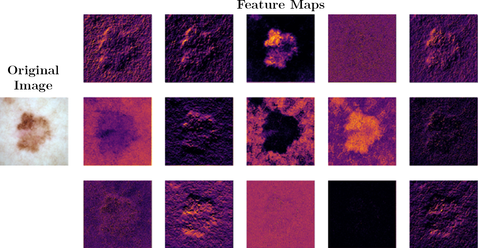![](https://github.com/anindox8/Ensemble-of-Multi-Scale-CNN-for-Dermatoscopy-Classification/blob/master/reports/images/imgnetplus_efn.png?raw=true)","execution_count":null},{"metadata":{"_uuid":"86e80d30-d1db-4407-8cb2-26e9d8582299","_cell_guid":"59dd11f4-fd75-462d-b252-f2474ddea6c4","trusted":true},"cell_type":"markdown","source":"**Features maps derived from the output of the second block of expanded convolutional layers in a finetuned EfficientNet-B6 initialized with ImageNet weights, after passing an input skin lesion image through the network.**","execution_count":null},{"metadata":{"_uuid":"f722497c-3ea6-4040-9da0-3b1ed0dfd495","_cell_guid":"9ed0a59f-283d-41c3-a3fb-a85f6bb1b36d","trusted":true},"cell_type":"markdown","source":"Thresholding is a very popular segmentation technique, used for separating an object considered as a foreground from its background. A threshold is a value which has two regions on its either side i.e. below the threshold or above the threshold.\nIn Computer Vision, this technique of thresholding is done on grayscale images. So initially, the image has to be converted in grayscale color space.","execution_count":null},{"metadata":{"_uuid":"cc5efdb1-0d16-4387-a181-f69a98d1fe70","_cell_guid":"744afb74-3983-4c8a-b48c-b773169d0c72","trusted":true},"cell_type":"code","source":"\n  \n# cv2.cvtColor is applied over the \n# image input with applied parameters \n# to convert the image in grayscale  \nimage = cv2.imread('../input/jpeg-melanoma-768x768/train/ISIC_0232101.jpg')\nimg = cv2.cvtColor(image, cv2.COLOR_BGR2GRAY) \n  \n# applying different thresholding  \n# techniques on the input image \n# all pixels value above 120 will  \n# be set to 255 \n\nret, thresh = cv2.threshold(img, 120, 255, cv2.THRESH_TOZERO) \n\n  \n# the window showing output images \n# with the corresponding thresholding  \n# techniques applied to the input images \nplt.imshow(thresh)","execution_count":null,"outputs":[]},{"metadata":{"_uuid":"2a50a13b-72a1-4625-b313-c886c8bf2ecf","_cell_guid":"4ec9f28c-365c-4ee9-bd55-3673aeb20e47","trusted":true},"cell_type":"markdown","source":"let's use dataloader from this awesome kernel [[Training CV] Melanoma Starter](https://www.kaggle.com/shonenkov/training-cv-melanoma-starter) of @shonenkov and vizualize some augmentations","execution_count":null},{"metadata":{"_uuid":"12727a23-7d2c-49dc-8747-7607fb6c73c1","_cell_guid":"51d4835d-7617-4476-a574-bab5f7fa6a80","trusted":true},"cell_type":"code","source":"df_meta = pd.read_csv('../input/melanoma-merged-external-data-512x512-jpeg/folds_13062020.csv')","execution_count":null,"outputs":[]},{"metadata":{"_uuid":"7d4dc00f-0543-4a2d-81b5-c7c98bf5a676","_cell_guid":"6ed1416c-0699-47ba-a56d-1a6e86db9988","trusted":true},"cell_type":"code","source":"df_meta.target.value_counts()","execution_count":null,"outputs":[]},{"metadata":{"_uuid":"acab59c7-b95e-4b44-aa78-bff903557cbc","_cell_guid":"5338cd40-291e-4448-9948-1e04700a332f","trusted":true},"cell_type":"code","source":"\ndef get_train_transforms():\n    return A.Compose([\n            A.RandomSizedCrop(min_max_height=(400, 400), height=512, width=512, p=0.5),\n            A.RandomRotate90(p=0.5),\n            A.HorizontalFlip(p=0.5),\n            A.VerticalFlip(p=0.5),\n            A.Resize(height=512, width=512, p=1),\n            A.Cutout(num_holes=8, max_h_size=64, max_w_size=64, fill_value=0, p=0.5),\n            ToTensorV2(p=1.0),                  \n        ], p=1.0)\n\ndef get_train_transforms1():\n    return A.Compose([\n\n            A.Resize(height=512, width=512, p=1),\n            A.Cutout(num_holes=8, max_h_size=64, max_w_size=64, fill_value=0, p=0.5),\n            ToTensorV2(p=1.0),                  \n        ], p=1.0)\n\ndef get_train_transforms2():\n    return A.Compose([\n\n            A.Resize(height=512, width=512, p=1),\n            A.CenterCrop(256, 256),\n            ToTensorV2(p=1.0),                  \n        ], p=1.0)\n\ndef get_valid_transforms():\n    return A.Compose([\n            A.Resize(height=512, width=512, p=1.0),\n            ToTensorV2(p=1.0),\n        ], p=1.0)\n\nDATA_PATH = '../input/melanoma-merged-external-data-512x512-jpeg'\nTRAIN_ROOT_PATH = f'{DATA_PATH}/512x512-dataset-melanoma/512x512-dataset-melanoma'\n\ndef onehot(size, target):\n    vec = torch.zeros(size, dtype=torch.float32)\n    vec[target] = 1.\n    return vec\n\nclass DatasetRetriever(Dataset):\n\n    def __init__(self, image_ids, labels, transforms=None):\n        super().__init__()\n        self.image_ids = image_ids\n        self.labels = labels\n        self.transforms = transforms\n\n    def __getitem__(self, idx: int):\n        image_id = self.image_ids[idx]\n        image = cv2.imread(f'{TRAIN_ROOT_PATH}/{image_id}.jpg', cv2.IMREAD_COLOR)\n        #plt.imshow(image)\n        #image = image.astype(np.float32) / 255.0\n\n        label = self.labels[idx]\n\n        if self.transforms:\n            sample = {'image': image}\n            sample = self.transforms(**sample)\n            image = sample['image']\n\n        target = onehot(2, label)\n        return image, target\n\n    def __len__(self) -> int:\n        return self.image_ids.shape[0]\n\n    def get_labels(self):\n        return list(self.labels)","execution_count":null,"outputs":[]},{"metadata":{"_uuid":"ee58e3d2-09fe-4135-86d1-bfc579416d72","_cell_guid":"c1598fb5-f027-400f-97dd-3e7847221284","trusted":true},"cell_type":"code","source":"\ndf_folds = pd.read_csv(f'{DATA_PATH}/folds.csv', index_col='image_id')\ntrain_dataset = DatasetRetriever(\n        image_ids=df_folds[df_folds['fold'] != 1].index.values,\n        labels=df_folds[df_folds['fold'] != 1].target.values,\n        transforms=get_train_transforms(),\n    )\n\ntrain_dataset1 = DatasetRetriever(\n        image_ids=df_folds[df_folds['fold'] != 1].index.values,\n        labels=df_folds[df_folds['fold'] != 1].target.values,\n        transforms=get_train_transforms1(),\n    )\ntrain_dataset2 = DatasetRetriever(\n        image_ids=df_folds[df_folds['fold'] != 1].index.values,\n        labels=df_folds[df_folds['fold'] != 1].target.values,\n        transforms=get_train_transforms2(),\n    )","execution_count":null,"outputs":[]},{"metadata":{"_uuid":"386ac626-ea85-4a71-b77c-f170efcfade1","_cell_guid":"2086a1c1-590e-461c-b047-723f3d239761","trusted":true},"cell_type":"markdown","source":"# Augmentations @shonenkov using in his kernel [[Training CV] Melanoma Starter](https://www.kaggle.com/shonenkov/training-cv-melanoma-starter)","execution_count":null},{"metadata":{"_uuid":"15a635bb-ba37-4034-9e35-1baadc08334d","_cell_guid":"667be039-9bc4-46f0-82d9-629261a84de3","trusted":true},"cell_type":"code","source":"image, label = train_dataset[0]\nplt.imshow(image.reshape(512,512,3))","execution_count":null,"outputs":[]},{"metadata":{"_uuid":"9925925b-ad25-4216-a5cd-b94a50289a5f","_cell_guid":"2a335129-5adc-4573-be9b-9102fa8e0518","trusted":true},"cell_type":"markdown","source":"# only cutout with 8 holes","execution_count":null},{"metadata":{"_uuid":"c133edd3-13d5-4e76-9c3b-3220e81d45bc","_cell_guid":"e48e0617-7b6d-4834-b3ae-b0c03cb2a7a9","trusted":true},"cell_type":"code","source":"image, label = train_dataset1[0]\nplt.imshow(image.reshape(512,512,3))","execution_count":null,"outputs":[]},{"metadata":{"_uuid":"9afc8de5-0625-4909-83b0-80537778fa95","_cell_guid":"8701340d-dfa4-4032-9d51-7ac23c3ecc41","trusted":true},"cell_type":"markdown","source":"# CenterCropping -> height = width = 256","execution_count":null},{"metadata":{"_uuid":"299abf1f-52a3-46ab-a160-e1b961e536cc","_cell_guid":"1f80d52a-b9d7-4cdd-b483-3b7fed029786","trusted":true},"cell_type":"code","source":"image, label = train_dataset2[0]\nplt.imshow(image.reshape(256,256,3))","execution_count":null,"outputs":[]},{"metadata":{"_uuid":"c981671e-9ebf-4c38-8fe3-a4ef804caee7","_cell_guid":"2278abaa-c4ab-499c-9384-63fb0eadaa32","trusted":true},"cell_type":"markdown","source":"# Data Augmentation with Generative Networks for Medical Imaging","execution_count":null},{"metadata":{"_uuid":"01f57eaf-d23a-4532-a98c-d8e72638c0ad","_cell_guid":"6cf448a1-1d01-4033-b655-3e02f9786bb0","trusted":true},"cell_type":"markdown","source":"**this is my first time with GAN, i can make mistakes very easily,correct  me if i am wrong :)**","execution_count":null},{"metadata":{"_uuid":"30392cec-e10f-4b83-9401-cc6059b677ae","_cell_guid":"2221b085-12b5-4322-a5f8-b9ce1cb7f494","trusted":true},"cell_type":"markdown","source":"i uploaded the weights from this awesome repo [lesion-GAN](https://github.com/alxiang/lesion-GAN)","execution_count":null},{"metadata":{"_uuid":"3bad86ab-a395-4c3d-835f-0c1e2367668d","_cell_guid":"10cd0711-6ccf-4d0a-b7c3-c8af4008a207","trusted":true},"cell_type":"markdown","source":"Dataset Link [lesion-GAN](https://www.kaggle.com/mobassir/ganweight)","execution_count":null},{"metadata":{"_uuid":"2c69dc80-45c2-44f9-be28-b86161b625eb","_cell_guid":"b02bfdc2-1f87-454d-8f78-9388c33b5c57","trusted":true},"cell_type":"markdown","source":"i am using those weights here for  testing and learning purposes  only :)","execution_count":null},{"metadata":{"_uuid":"73a6d634-77ec-41b7-81bc-b28975c008ab","_cell_guid":"98ee58ad-6e69-49ca-9ae9-fec83ed3e303","trusted":true},"cell_type":"markdown","source":"the weight file we  are gonna use,implements this awesome paper [**Towards Interpretable Skin Lesion Classification with Deep Learning Models**](https://www.ncbi.nlm.nih.gov/pmc/articles/PMC7153112/pdf/3203149.pdf)","execution_count":null},{"metadata":{"_uuid":"368a87fd-1eff-4d78-b51a-b98fce5304d4","_cell_guid":"6bd2aaf4-fdfb-4e4d-af13-5d8d35076688","trusted":true},"cell_type":"markdown","source":"ABSTRACT from that paper : \n\nSkin disease is a prevalent condition all over the world. Computer vision-based technology for automatic skin lesion\nclassification holds great promise as an effective screening tool for early diagnosis. In this paper, we propose an\naccurate and interpretable deep learning pipeline to achieve such a goal. Comparing with existing research, we would\nlike to highlight the following aspects of our model. 1) Rather than a single model, our approach ensembles a set of\ndeep learning architectures to achieve better classification accuracy; 2) Generative adversarial network (GAN) is\ninvolved in the model training to promote data scale and diversity; 3) Local interpretable model-agnostic explanation\n(LIME) strategy is applied to extract evidence from the skin images to support the classification results. Our\nexperimental results on real-world skin image corpus demonstrate the effectiveness and robustness of our method.\nThe explainability of our model further enhances its applicability in real clinical practice.","execution_count":null},{"metadata":{"_uuid":"83388768-a535-4862-a6eb-94523b822f0d","_cell_guid":"9c4b4758-e35b-44cc-b957-b2af4e0365d8","trusted":true},"cell_type":"code","source":"import os\nos.listdir('../input/ganweight')","execution_count":null,"outputs":[]},{"metadata":{"_uuid":"ba8ef6a3-6085-4810-8e47-f5dc4dd4c813","_cell_guid":"b8610fc4-5385-43e1-bd64-43ee306b8af5","trusted":true},"cell_type":"markdown","source":"# so what is GAN and  why should we care?","execution_count":null},{"metadata":{"_uuid":"89d57e58-ec21-42f3-a2d7-1ac13cf1a5df","_cell_guid":"3bc2a453-fa2e-40a5-ad4c-2004cd955b72","trusted":true},"cell_type":"markdown","source":"Generative Adversarial Networks (GAN) were first introduced by Ian Goodfellow et al, in 2014 (https://papers.nips.cc/paper/5423-generative-adversarial-nets.pdf).\n\nIt was shown that random handwritten digits could be generated from the generator network of a GAN, after training on the MNIST dataset (http://yann.lecun.com/exdb/mnist/).","execution_count":null},{"metadata":{"_uuid":"f9c34459-89ba-4e30-b229-a3f4279b4a7d","_cell_guid":"e3f280f0-84fa-4232-ab3f-798260b2d6b2","trusted":true},"cell_type":"markdown","source":"# Lets begin remembering how GANs work:\n\nThe idea behind GANs is that you have two networks, a generator $G$ and a discriminator $D$, competing against each other. The generator makes \"fake\" data to pass to the discriminator. The discriminator also sees real training data and predicts if the data it's received is real or fake.\n\nThe generator is trained to fool the discriminator, it wants to output data that looks as close as possible to real, training data.\nThe discriminator is a classifier that is trained to figure out which data is real and which is fake.\nWhat ends up happening is that the generator learns to make data that is indistinguishable from real data to the discriminator.\n\n![](https://i.ibb.co/jkZPNyz/ref.png)\n\nThe general structure of the GAN that we are using here is shown in the diagram above. The latent sample is a random vector that the generator uses to construct its fake images. This is often called a latent vector and that vector space is called latent space. As the generator trains, it figures out how to map latent vectors to recognizable images that can fool the discriminator.\n\nOnce the generator has trained, we can throw out the discriminator after we are done with training.","execution_count":null},{"metadata":{"_uuid":"b3189207-5998-4179-a9a2-d7a76e7f5af5","_cell_guid":"4a19f735-69e0-4de5-8f67-836c912ea5b1","trusted":true},"cell_type":"code","source":"img = cv2.imread('../input/melanoma-merged-external-data-512x512-jpeg/512x512-dataset-melanoma/512x512-dataset-melanoma/ISIC_4568001.jpg')","execution_count":null,"outputs":[]},{"metadata":{"_uuid":"b28ab702-cf4a-40a0-b627-473503e018fd","_cell_guid":"a5c25ed9-065a-49b7-a143-e2b7d9dcfbd7","trusted":true},"cell_type":"code","source":"img.shape","execution_count":null,"outputs":[]},{"metadata":{"_uuid":"bfea0c92-8592-435e-9ea8-7f5756e6d4a1","_cell_guid":"3bb4914a-758c-40cf-b5df-41988531543b","trusted":true},"cell_type":"code","source":"\njson_file = open('../input/ganweight/generator.json', 'r')\ngenerator_json = json_file.read()\njson_file.close()\ngenerator = model_from_json(generator_json)\ngenerator.load_weights('../input/ganweight/generator_weights.hdf5')","execution_count":null,"outputs":[]},{"metadata":{"_uuid":"c62ad6eb-1f37-4e46-aec5-6e0f71c07077","_cell_guid":"0865164b-b3ac-470e-b2b4-492f346ab4ab","trusted":true},"cell_type":"code","source":"plt.imshow(img[:,:,1])","execution_count":null,"outputs":[]},{"metadata":{"_uuid":"9e127cb4-64bd-4e2c-9297-5389e0d19952","_cell_guid":"9279a94c-2f0e-4d28-88c9-4b0795ef1793","trusted":true},"cell_type":"code","source":"originals = img\n\n#data = np.load(\".../HAMNOAUG_256.npz\")\n\n#labels = 1\n\n#temp = np.empty((0, 128, 128, 3))\nfor i in range(originals.shape[0]):\n    temp_r = skimage.measure.block_reduce(originals[:,:,0], (4,4), np.mean) # (4,4) = factor of reduction\n    temp_g = skimage.measure.block_reduce(originals[:,:,1], (4,4), np.mean)\n    temp_b = skimage.measure.block_reduce(originals[:,:,2], (4,4), np.mean)\n    temp_rgb = np.stack([temp_r, temp_g, temp_b], axis=-1)\n\n    #temp[i] = temp_rgb    \noriginals = temp_rgb\noriginals /= 255","execution_count":null,"outputs":[]},{"metadata":{"_uuid":"ad3aa075-a509-4bfb-8b26-840a36b66bba","_cell_guid":"00aaedfb-3c86-4adf-8563-3cc216a31964","trusted":true},"cell_type":"code","source":"nn_sampled_labels = np.concatenate([np.zeros(3), np.ones(3), np.ones(3)+1])\nnn_noise = np.random.normal(0, 1, (9, 128))","execution_count":null,"outputs":[]},{"metadata":{"_uuid":"28e8fe36-f311-46d8-a27a-49295b6c5414","_cell_guid":"6460e459-1b57-41e8-bc3d-e38d4eff515c","trusted":true},"cell_type":"code","source":"gen_imgs = 0.5*generator.predict([nn_noise, nn_sampled_labels]) + 0.5","execution_count":null,"outputs":[]},{"metadata":{"_uuid":"3b1b8465-13e6-4a9c-890c-b865163f26dd","_cell_guid":"253e8de1-6e2d-4a0b-91e7-fa06fac0bf9f","trusted":true},"cell_type":"code","source":"originals.shape","execution_count":null,"outputs":[]},{"metadata":{"_uuid":"18926936-ffb5-48c3-b30e-e3d0cb1fd01f","_cell_guid":"07b6c2d5-7c01-4983-8781-a6b56e8b2f17","trusted":true},"cell_type":"markdown","source":"# Original","execution_count":null},{"metadata":{"_uuid":"1a9a43ba-5af3-4bc5-be51-2fe743010b2d","_cell_guid":"8b0e5527-6e61-4316-8e33-91ffdb99e660","trusted":true},"cell_type":"code","source":"plt.imshow(img)","execution_count":null,"outputs":[]},{"metadata":{"_uuid":"733369fd-537e-4138-acf3-816fd0dfdd88","_cell_guid":"7e29f583-7e14-4869-a163-8b9057e30ff2","trusted":true},"cell_type":"markdown","source":"# Fake Images :)","execution_count":null},{"metadata":{"_uuid":"be8da2fd-2f7f-42a6-81e3-6c4a07bbc8eb","_cell_guid":"7330353e-b493-4f3b-ac89-baa2a83588d9","trusted":true},"cell_type":"code","source":"n_row = 3\nn_col = 3\n_, axs = plt.subplots(n_row, n_col, figsize=(15, 15))\naxs = axs.flatten()\n\nfor i in range(9):\n    axs[i].imshow(gen_imgs[i])\nplt.show()","execution_count":null,"outputs":[]},{"metadata":{"_uuid":"f8fd5d6e-8dd9-42fb-90e8-240ccc3c53c1","_cell_guid":"50e5f8c9-2252-4ee5-9583-f057bf4b271d","trusted":true},"cell_type":"markdown","source":"you can play with the models implementation from here [ACGAN](https://github.com/alxiang/lesion-GAN/blob/master/ACGAN.ipynb) and probably want to convert it into pytorch. because **THERE IS NOTHING LIKE PYTORCH.** 😊\n\n**PYTORCH IS** ❤️❤️❤️","execution_count":null},{"metadata":{"_uuid":"adf744d1-5e4e-48f4-a0b2-40fdf72fa628","_cell_guid":"4b538fb7-c74f-4b15-8c92-ad4d09db30df","trusted":true},"cell_type":"markdown","source":"# Thank You For Reading :)","execution_count":null},{"metadata":{"_uuid":"9aec1fbe-4b7f-4f5e-9f70-984f8afea859","_cell_guid":"17b4d30c-46ec-424c-a913-7c7642acf72f","trusted":true},"cell_type":"markdown","source":"ঈদ মোবারক😊","execution_count":null},{"metadata":{"_uuid":"0518562b-eea0-488a-bf78-b2c69ce3ee78","_cell_guid":"a1dac584-2dd7-4ab1-a65b-04dfa0db3ddc","trusted":true},"cell_type":"code","source":"","execution_count":null,"outputs":[]}],"metadata":{"kernelspec":{"language":"python","display_name":"Python 3","name":"python3"},"language_info":{"pygments_lexer":"ipython3","nbconvert_exporter":"python","version":"3.6.4","file_extension":".py","codemirror_mode":{"name":"ipython","version":3},"name":"python","mimetype":"text/x-python"}},"nbformat":4,"nbformat_minor":4}