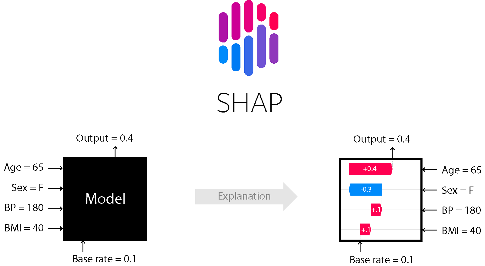
\n\n#### About SHAP from [the reposiroty](https://github.com/slundberg/shap)\n
\n\n#### SHAP (SHapley Additive exPlanations) is a game theoretic approach to explain the output of any machine learning model. It connects optimal credit allocation with local explanations using the classic Shapley values from game theory and their related extensions.","execution_count":null},{"metadata":{},"cell_type":"markdown","source":"## Dependencies","execution_count":null},{"metadata":{"_uuid":"8f2839f25d086af736a60e9eeb907d3b93b6e0e5","_cell_guid":"b1076dfc-b9ad-4769-8c92-a6c4dae69d19","trusted":true,"_kg_hide-input":true},"cell_type":"code","source":"!pip install --quiet image-classifiers\n\nimport warnings, json, re, glob, math, shutil, os, shap\nimport numpy as np\nimport pandas as pd\nimport seaborn as sns\nimport matplotlib.pyplot as plt\nimport tensorflow as tf\nimport tensorflow.keras.layers as L\nimport tensorflow.keras.backend as K\nfrom tensorflow.keras.preprocessing.image import ImageDataGenerator\nfrom tensorflow.keras import Model\nfrom kaggle_datasets import KaggleDatasets\nfrom sklearn.model_selection import KFold\nfrom classification_models.tfkeras import Classifiers\n\nSEED = 0\nwarnings.filterwarnings(\"ignore\")","execution_count":null,"outputs":[]},{"metadata":{},"cell_type":"markdown","source":"# Load data","execution_count":null},{"metadata":{"_uuid":"d629ff2d2480ee46fbb7e2d37f6b5fab8052498a","_cell_guid":"79c7e3d0-c299-4dcb-8224-4455121ee9b0","trusted":true,"_kg_hide-input":true},"cell_type":"code","source":"database_base_path = '/kaggle/input/siim-isic-melanoma-classification/'\ntrain = pd.read_csv(database_base_path + 'train.csv')\ntest = pd.read_csv(database_base_path + 'test.csv')\n\nprint('Train samples: %d' % len(train))\ndisplay(train.head())\nprint(f'Test samples: {len(test)}')\ndisplay(test.head())\n\n# pre-process data\ntrain['image_name'] = train['image_name'].apply(lambda x: x + '.jpg')\ntrain['target'] = train['target'].astype(str)\n\nGCS_PATH = KaggleDatasets().get_gcs_path('melanoma-256x256')\nTRAINING_FILENAMES = tf.io.gfile.glob(GCS_PATH + '/train*.tfrec')\nTEST_FILENAMES = tf.io.gfile.glob(GCS_PATH + '/test*.tfrec')","execution_count":null,"outputs":[]},{"metadata":{},"cell_type":"markdown","source":"## Parameters","execution_count":null},{"metadata":{"trusted":true,"_kg_hide-input":false},"cell_type":"code","source":"HEIGHT = 256\nWIDTH = 256\nCHANNELS = 3\nBATCH_SIZE = 64\nAUTO = tf.data.experimental.AUTOTUNE\n\n# SHAP parameters\nimages_to_explain = ['ISIC_0074311.jpg', 'ISIC_0074542.jpg', 'ISIC_0075663.jpg', 'ISIC_0075914.jpg', \n 'ISIC_0076262.jpg', 'ISIC_0082543.jpg', 'ISIC_0082934.jpg', 'ISIC_0083035.jpg', \n 'ISIC_0084086.jpg', 'ISIC_0084270.jpg', 'ISIC_0149568.jpg', 'ISIC_0188432.jpg', \n 'ISIC_0207268.jpg', 'ISIC_0232101.jpg', 'ISIC_0247330.jpg', 'ISIC_0528044.jpg', \n 'ISIC_1219894.jpg', 'ISIC_2776906.jpg']\n\neval_df = train[train['image_name'].isin(images_to_explain)]\n\nos.makedirs('to_explain/')\nfor filename in images_to_explain:\n shutil.copy('/kaggle/input/siim-isic-melanoma-classification/jpeg/train/' + filename, 'to_explain/')","execution_count":null,"outputs":[]},{"metadata":{},"cell_type":"markdown","source":"## Auxiliary functions","execution_count":null},{"metadata":{"_kg_hide-input":true,"trusted":true},"cell_type":"code","source":"# Datasets utility functions\nUNLABELED_TFREC_FORMAT = {\n \"image\": tf.io.FixedLenFeature([], tf.string), # tf.string means bytestring\n \"image_name\": tf.io.FixedLenFeature([], tf.string), # shape [] means single element\n # meta features\n \"patient_id\": tf.io.FixedLenFeature([], tf.int64),\n \"sex\": tf.io.FixedLenFeature([], tf.int64),\n \"age_approx\": tf.io.FixedLenFeature([], tf.int64),\n \"anatom_site_general_challenge\": tf.io.FixedLenFeature([], tf.int64),\n}\n\ndef decode_image(image_data, height, width, channels):\n image = tf.image.decode_jpeg(image_data, channels=channels)\n image = tf.cast(image, tf.float32) / 255.0\n image = tf.reshape(image, [height, width, channels])\n return image\n\n# Test function\ndef read_unlabeled_tfrecord(example, height=HEIGHT, width=WIDTH, channels=CHANNELS):\n example = tf.io.parse_single_example(example, UNLABELED_TFREC_FORMAT)\n image = decode_image(example['image'], height, width, channels)\n image_name = example['image_name']\n # meta features\n data = {}\n data['patient_id'] = tf.cast(example['patient_id'], tf.int32)\n data['sex'] = tf.cast(example['sex'], tf.int32)\n data['age_approx'] = tf.cast(example['age_approx'], tf.int32)\n data['anatom_site_general_challenge'] = tf.cast(tf.one_hot(example['anatom_site_general_challenge'], 7), tf.int32)\n \n return {'input_image': image, 'input_tabular': data}, image_name # returns a dataset of (image, data, image_name)\n\ndef load_dataset_test(filenames, buffer_size=-1):\n dataset = tf.data.TFRecordDataset(filenames, num_parallel_reads=buffer_size) # automatically interleaves reads from multiple files\n dataset = dataset.map(read_unlabeled_tfrecord, num_parallel_calls=buffer_size)\n # returns a dataset of (image, data, label, image_name) pairs if labeled=True or (image, data, image_name) pairs if labeled=False\n return dataset\n\ndef get_test_dataset(filenames, batch_size=32, buffer_size=-1):\n dataset = load_dataset_test(filenames, buffer_size=buffer_size)\n dataset = dataset.batch(batch_size, drop_remainder=False)\n dataset = dataset.prefetch(buffer_size)\n return dataset\n\n# Custom SHAP plot\ndef image_plot(shap_values, pixel_values, labels=None, preds=None, names=None, width=20, aspect=0.2, hspace=0.2, labelpad=None, show=True, fig_size=None):\n \"\"\" Plots SHAP values for image inputs.\n Parameters\n ----------\n shap_values : [numpy.array]\n List of arrays of SHAP values. Each array has the shap (# samples x width x height x channels), and the\n length of the list is equal to the number of model outputs that are being explained.\n pixel_values : numpy.array\n Matrix of pixel values (# samples x width x height x channels) for each image. It should be the same\n shape as each array in the shap_values list of arrays.\n labels : list\n List of names for each of the model outputs that are being explained. This list should be the same length\n as the shap_values list.\n width : float\n The width of the produced matplotlib plot.\n labelpad : float\n How much padding to use around the model output labels.\n show : bool\n Whether matplotlib.pyplot.show() is called before returning. Setting this to False allows the plot\n to be customized further after it has been created.\n \"\"\"\n\n multi_output = True\n if type(shap_values) != list:\n multi_output = False\n shap_values = [shap_values]\n\n # make sure labels\n if labels is not None:\n assert labels.shape[0] == shap_values[0].shape[0], \"Labels must have same row count as shap_values arrays!\"\n if multi_output:\n assert labels.shape[1] == len(shap_values), \"Labels must have a column for each output in shap_values!\"\n else:\n assert len(labels.shape) == 1, \"Labels must be a vector for single output shap_values.\"\n\n label_kwargs = {} if labelpad is None else {'pad': labelpad}\n\n # plot our explanations\n x = pixel_values\n if fig_size is None:\n fig_size = np.array([3 * (len(shap_values) + 1), 2.5 * (x.shape[0] + 1)])\n if fig_size[0] > width:\n fig_size *= width / fig_size[0]\n fig, axes = plt.subplots(nrows=x.shape[0], ncols=len(shap_values) + 1, figsize=fig_size)\n if len(axes.shape) == 1:\n axes = axes.reshape(1,axes.size)\n for row in range(x.shape[0]):\n x_curr = x[row].copy()\n\n # make sure\n if len(x_curr.shape) == 3 and x_curr.shape[2] == 1:\n x_curr = x_curr.reshape(x_curr.shape[:2])\n if x_curr.max() > 1:\n x_curr /= 255.\n\n # get a grayscale version of the image\n if len(x_curr.shape) == 3 and x_curr.shape[2] == 3:\n x_curr_gray = (0.2989 * x_curr[:,:,0] + 0.5870 * x_curr[:,:,1] + 0.1140 * x_curr[:,:,2]) # rgb to gray\n else:\n x_curr_gray = x_curr\n\n axes[row,0].imshow(x_curr, cmap=plt.get_cmap('gray'))\n axes[row,0].set_title(f'Image: {names[row]}', **label_kwargs)\n axes[row,0].axis('off')\n if len(shap_values[0][row].shape) == 2:\n abs_vals = np.stack([np.abs(shap_values[i]) for i in range(len(shap_values))], 0).flatten()\n else:\n abs_vals = np.stack([np.abs(shap_values[i].sum(-1)) for i in range(len(shap_values))], 0).flatten()\n max_val = np.nanpercentile(abs_vals, 99.9)\n for i in range(len(shap_values)):\n if labels is not None:\n axes[row,i+1].set_title(f'Label: {labels[row,i]} Pred: {preds[row,i]:.2f}', **label_kwargs)\n sv = shap_values[i][row] if len(shap_values[i][row].shape) == 2 else shap_values[i][row].sum(-1)\n axes[row,i+1].imshow(x_curr_gray, cmap=plt.get_cmap('gray'), alpha=0.15, extent=(-1, sv.shape[1], sv.shape[0], -1))\n im = axes[row,i+1].imshow(sv, cmap=shap.plots.colors.red_transparent_blue, vmin=-max_val, vmax=max_val)\n axes[row,i+1].axis('off')\n if hspace == 'auto':\n fig.tight_layout()\n else:\n fig.subplots_adjust(hspace=hspace)\n cb = fig.colorbar(im, ax=np.ravel(axes).tolist(), label=\"SHAP value\", orientation=\"horizontal\", aspect=fig_size[0]/aspect)\n cb.outline.set_visible(False)\n if show:\n plt.show()","execution_count":null,"outputs":[]},{"metadata":{},"cell_type":"markdown","source":"# Model\n\n### I will be using a ResNet18 model, trained with 3-Fold data.","execution_count":null},{"metadata":{"trusted":true},"cell_type":"code","source":"def model_fn(input_shape):\n input_image = L.Input(shape=input_shape, name='input_image')\n ResNet18, preprocess_input = Classifiers.get('resnet18')\n base_model = ResNet18(input_shape=input_shape, \n weights=None, \n include_top=False)\n\n x = base_model(input_image)\n x = L.GlobalAveragePooling2D()(x)\n output = L.Dense(1, activation='sigmoid')(x)\n \n model = Model(inputs=input_image, outputs=output)\n \n return model\n\nmodel = model_fn((HEIGHT, WIDTH, CHANNELS))\nmodel.load_weights('/kaggle/input/shap-model/ResNet_18.h5') # load pre-trained weights\nmodel.summary()","execution_count":null,"outputs":[]},{"metadata":{},"cell_type":"markdown","source":"# First lets make the evaluated set predictions","execution_count":null},{"metadata":{"trusted":true},"cell_type":"code","source":"# data generator\neval_datagen = ImageDataGenerator(rescale=1./255)\n\neval_generator=eval_datagen.flow_from_dataframe(\n dataframe=eval_df,\n directory='to_explain/',\n x_col='image_name',\n y_col='target',\n class_mode='binary', \n batch_size=BATCH_SIZE, \n target_size=(HEIGHT, WIDTH),\n shuffle=False,\n seed=SEED)\n\n# add predictions\neval_df['preds'] = model.predict(eval_generator)\ndisplay(eval_df.head())","execution_count":null,"outputs":[]},{"metadata":{},"cell_type":"markdown","source":"# SHAP model explainability\n\n### For this experiment we will use `GradientExplainer`, below is an example from the Imagenet dataset applied to a VGG16 model.\n\n#### The more `pink` each pixel is the more it contributes to the image being classified on a specific class, and the more `blue` it is more the pixel contributes for it not being of that class. \n\n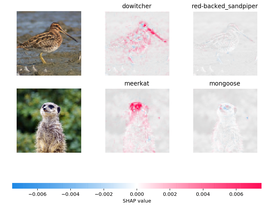\n\n#### Above for the 1st image the beak and wings of the dowitcher had a big contribution on assigning it to the correct class, and for the 2nd image the face of the meerkat contributed a lot to correctly classify it, for those examples we can assume that the model is doing a good job.","execution_count":null},{"metadata":{},"cell_type":"markdown","source":"# Below are the images that will be explained by SHAP, you can also see the label and the model's prediction for each image.","execution_count":null},{"metadata":{"_kg_hide-input":true,"trusted":true},"cell_type":"code","source":"n_explain = 18\neval_generator.batch_size = n_explain # background dataset\nbackground, lbls = next(eval_generator)\nlbls = lbls.reshape(lbls.shape[0], 1)\n\nfig, axes = plt.subplots(6, 3, figsize=(20, 14))\naxes = axes.flatten()\nfor x in range(6):\n axes[x].imshow(background[x])\n axes[x+6].imshow(background[x+6])\n axes[x+12].imshow(background[x+12])\n \n axes[x].set_title(f\"Image {eval_df['image_name'].values[x]}, Label: {eval_df['target'].values[x]}, Pred: {eval_df['preds'].values[x]:.2f}\")\n axes[x+6].set_title(f\"Image {eval_df['image_name'].values[x+6]}, Label: {eval_df['target'].values[x+6]}, Pred: {eval_df['preds'].values[x+6]:.2f}\")\n axes[x+12].set_title(f\"Image {eval_df['image_name'].values[x+12]}, Label: {eval_df['target'].values[x+12]}, Pred: {eval_df['preds'].values[x+12]:.2f}\")\n \n axes[x].set_axis_off()\n axes[x+6].set_axis_off()\n axes[x+12].set_axis_off()\n \nplt.show()","execution_count":null,"outputs":[]},{"metadata":{},"cell_type":"markdown","source":"As we can see the model missed all the predictions that the label was 1, we will also see the explanation for those images.","execution_count":null},{"metadata":{},"cell_type":"markdown","source":"# Using SHAP to explain the images","execution_count":null},{"metadata":{"trusted":true,"_kg_hide-input":true},"cell_type":"code","source":"# explain predictions of the model on \"n_explain\" images\ne = shap.GradientExplainer(model, background)\nshap_values = e.shap_values(background)\n\n# plot the feature attributions\nimage_plot(shap_values, background[:10], labels=lbls, preds=eval_df['preds'].values[:10].reshape(10, 1), names=eval_df['image_name'].values[:10], \n hspace=0.2, fig_size=(20, 40))","execution_count":null,"outputs":[]},{"metadata":{},"cell_type":"markdown","source":"At all the above images the prediction score was very low, which resulted in the explained images (right images) being mostly gray, if you look really close, you may see some pink dots. At the same time, we can notice that at least the model pays attention mainly to the skin marks.\n\nOne interesting thing here is that the model seems to do not care about hair or the mm scale.","execution_count":null},{"metadata":{},"cell_type":"markdown","source":"# Now the explanation for the positive images","execution_count":null},{"metadata":{"trusted":true,"_kg_hide-input":true},"cell_type":"code","source":"shap_values_positive = shap.GradientExplainer(model, background[10:15]).shap_values(background[10:15])\n\n# plot the feature attributions\nimage_plot(shap_values_positive, background[10:15], labels=lbls[10:15], preds=eval_df['preds'].values[10:15].reshape(5, 1), \n names=eval_df['image_name'].values[10:15], fig_size=(20, 20))","execution_count":null,"outputs":[]},{"metadata":{},"cell_type":"markdown","source":"Here on the positive images you can see much more pink dots, they mean that those pixels contributed to the class 1 prediction, even if the model did not predicted the images as class 1, some part of the images weighted on that direction.\n\n- In this 1st image the model really messed, it gave attention to a part of the image that did not even had a skin mark.\n- At the 4th image (ISIC_0232101) the model gave some attention to the mm scale, and also scattered some attention across the image, not focussing on the skin marg too much.\n\n### Looking at those images it is clear that the model has a lot to learn about the positive classes.\n\n#### If you liked this experiment leave a comment below I may update it with a better model or make another version with both image and tabular data.","execution_count":null},{"metadata":{},"cell_type":"markdown","source":"# Images that were predicted as postive or were very close","execution_count":null},{"metadata":{"trusted":true},"cell_type":"code","source":"shap_values_positive = shap.GradientExplainer(model, background[-3:]).shap_values(background[-3:])\n\n# plot the feature attributions\nimage_plot(shap_values_positive, background[-3:], labels=lbls[-3:], preds=eval_df['preds'].values[-3:].reshape(3, 1), \n names=eval_df['image_name'].values[-3:], fig_size=(20, 20))","execution_count":null,"outputs":[]},{"metadata":{},"cell_type":"markdown","source":"One very interesting part here is that the \"microscope\" effect does not seems to impact the predictions.\n\n- On the 1st image the model focused more on the skin mark that was more red, and cared less about the brown mark at the side.\n- This 2nd image is actually a negative sample but was almost predicted as positive, the model gave a lot of attention to the center.\n- On the 3rd image that purple stain did not really mattered to the model.\n\nIt seems that the microscope augmentation that was suggested at the forum could be applied, at least this model did not use the circle to bias the prediction. Also, all 3 images had the `mm scale` but the model did not really care about it.","execution_count":null},{"metadata":{},"cell_type":"markdown","source":"# Test set predictions","execution_count":null},{"metadata":{"_kg_hide-input":true,"trusted":true},"cell_type":"code","source":"test_dataset = get_test_dataset(TEST_FILENAMES, batch_size=BATCH_SIZE, buffer_size=AUTO)\nimage_names = next(iter(test_dataset.unbatch().map(lambda data, image_name: image_name).batch(len(test)))).numpy().astype('U')\n\ntest_preds = model.predict(test_dataset)\n\nname_preds = dict(zip(image_names, test_preds.reshape(len(test_preds))))\ntest['target'] = test.apply(lambda x: name_preds[x['image_name']], axis=1)\n\n\nprint(f\"Test predictions {len(test[test['target'] > .5])}|{len(test[test['target'] <= .5])}\")\nprint('Top 10 samples')\ndisplay(test[['image_name', 'sex', 'age_approx','anatom_site_general_challenge','target']].head(10))\n\nprint('Top 10 positive samples')\ndisplay(test[['image_name', 'sex', 'age_approx','anatom_site_general_challenge', 'target']].query('target > .5').head(10))\n\n\nsubmission = pd.read_csv(database_base_path + 'sample_submission.csv')\nsubmission['target'] = test['target']\nsubmission.to_csv('submission.csv', index=False)","execution_count":null,"outputs":[]}],"metadata":{"kernelspec":{"language":"python","display_name":"Python 3","name":"python3"},"language_info":{"pygments_lexer":"ipython3","nbconvert_exporter":"python","version":"3.6.4","file_extension":".py","codemirror_mode":{"name":"ipython","version":3},"name":"python","mimetype":"text/x-python"}},"nbformat":4,"nbformat_minor":4}