Table of Contents
\n What is Melanoma?1\n Studying the data2\n Exploratory Data Analysis3\n Resizing the Images4 \n Extract features from Images5 \n Train the model and predict the result6\n\nReferences:
\nI would like to thank [Grandmaster Dieter](https://www.kaggle.com/christofhenkel) for sharing this awesome kernel to extract features from Images using a pretrained NN. Here's a link to his kernel:-\nhttps://www.kaggle.com/christofhenkel/extract-image-features-from-pretrained-nn","execution_count":null},{"metadata":{"_uuid":"8f2839f25d086af736a60e9eeb907d3b93b6e0e5","_cell_guid":"b1076dfc-b9ad-4769-8c92-a6c4dae69d19","trusted":true,"_kg_hide-input":true,"_kg_hide-output":true},"cell_type":"code","source":"import pandas as pd\nimport numpy as np\nimport plotly.graph_objects as go\nfrom plotly.subplots import make_subplots\nimport plotly_express as px\nimport matplotlib.pyplot as plt\nimport seaborn as sns\nimport cv2\nimport os\nfrom tqdm import tqdm, tqdm_notebook\nimport gc\nimport warnings\nwarnings.filterwarnings(\"ignore\")\n\nfrom sklearn.preprocessing import LabelEncoder\nfrom sklearn.model_selection import StratifiedKFold\nfrom sklearn.metrics import roc_auc_score, roc_curve\nfrom keras.applications.densenet import preprocess_input, DenseNet121\nfrom keras.models import Model\nfrom keras.layers import GlobalAveragePooling2D, Input, Lambda, AveragePooling1D\nimport keras.backend as K\nfrom lightgbm import LGBMClassifier","execution_count":null,"outputs":[]},{"metadata":{},"cell_type":"markdown","source":"# 1. What is Melanoma?\nGo back to Table of Contents\n## -> Overview\n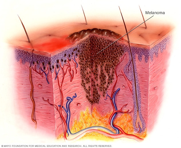 \nMelanoma, the most serious type of skin cancer, develops in the cells (melanocytes) that produce melanin — the pigment that gives your skin its color. Melanoma can also form in your eyes and, rarely, inside your body, such as in your nose or throat.\n\nThe exact cause of all melanomas isn't clear, but exposure to ultraviolet (UV) radiation from sunlight or tanning lamps and beds increases your risk of developing melanoma. Limiting your exposure to UV radiation can help reduce your risk of melanoma.\n\nThe risk of melanoma seems to be increasing in people under 40, especially women. Knowing the warning signs of skin cancer can help ensure that cancerous changes are detected and treated before the cancer has spread. Melanoma can be treated successfully if it is detected early.\n## -> Symptoms\nMelanomas can develop anywhere on your body. They most often develop in areas that have had exposure to the sun, such as your back, legs, arms and face.\n\nMelanomas can also occur in areas that don't receive much sun exposure, such as the soles of your feet, palms of your hands and fingernail beds. These hidden melanomas are more common in people with darker skin.\n\nThe first melanoma signs and symptoms often are:\n\nA change in an existing mole\nThe development of a new pigmented or unusual-looking growth on your skin\nMelanoma doesn't always begin as a mole. It can also occur on otherwise normal-appearing skin.\n## -> Causes\n
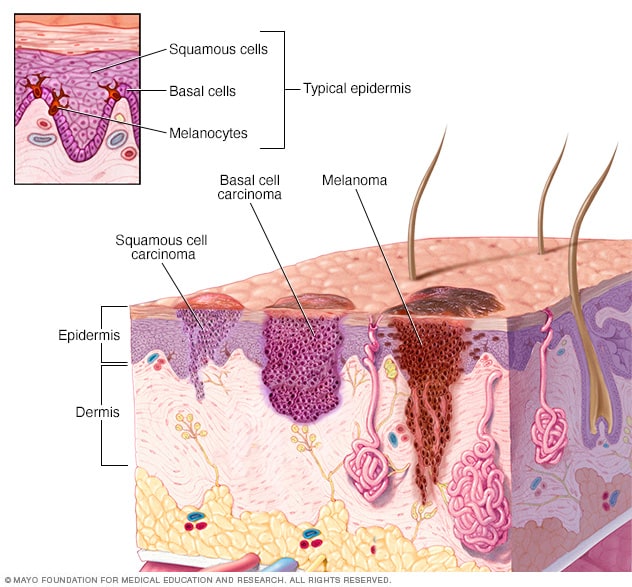 \nMelanoma occurs when something goes wrong in the melanin-producing cells (melanocytes) that give color to your skin.\n\nNormally, skin cells develop in a controlled and orderly way — healthy new cells push older cells toward your skin's surface, where they die and eventually fall off. But when some cells develop DNA damage, new cells may begin to grow out of control and can eventually form a mass of cancerous cells.\n\nJust what damages DNA in skin cells and how this leads to melanoma isn't clear. It's likely that a combination of factors, including environmental and genetic factors, causes melanoma. Still, doctors believe exposure to ultraviolet (UV) radiation from the sun and from tanning lamps and beds is the leading cause of melanoma.\n\nUV light doesn't cause all melanomas, especially those that occur in places on your body that don't receive exposure to sunlight. This indicates that other factors may contribute to your risk of melanoma.","execution_count":null},{"metadata":{},"cell_type":"markdown","source":"# 2. Studying the data\nGo back to Table of Contents\n\nIn this section, I'll fetch the train and test data and study their distributions. Interestingly, this competition has both tabular as well as image data. So, I will be extracting the features from Images and then combine it with the tabular data and then make the predictions.","execution_count":null},{"metadata":{"_uuid":"d629ff2d2480ee46fbb7e2d37f6b5fab8052498a","_cell_guid":"79c7e3d0-c299-4dcb-8224-4455121ee9b0","trusted":true,"_kg_hide-input":true},"cell_type":"code","source":"df_train = pd.read_csv('/kaggle/input/siim-isic-melanoma-classification/train.csv')\ndf_test = pd.read_csv('/kaggle/input/siim-isic-melanoma-classification/test.csv')","execution_count":null,"outputs":[]},{"metadata":{"trusted":true,"_kg_hide-input":true,"_kg_hide-output":true},"cell_type":"code","source":"display(df_train.info())\ndisplay(df_test.info())","execution_count":null,"outputs":[]},{"metadata":{"trusted":true,"_kg_hide-input":true},"cell_type":"code","source":"print('No of patients in train set(A): {}'.format(len(df_train.patient_id.unique().tolist())))\nprint('No of patients in test set(B): {}'.format(len(df_test.patient_id.unique().tolist())))\nprint('No of patients that are in train set but not test set(A-B): {}'.format(len(set(df_train.patient_id.unique()) - set(df_test.patient_id.unique()))))\nprint('No of patients that are in test set but not train set(B-A): {}'.format(len(set(df_test.patient_id.unique()) - set(df_train.patient_id.unique()))))\nprint('*'*64)\nprint('No of images in train set(C): {}'.format(len(df_train.image_name.unique().tolist())))\nprint('No of images in test set(D): {}'.format(len(df_test.image_name.unique().tolist())))\nprint('No of images that are in train set but not test set(C-D): {}'.format(len(set(df_train.image_name.unique()) - set(df_test.image_name.unique()))))\nprint('No of images that are in test set but not train set(D-C): {}'.format(len(set(df_test.image_name.unique()) - set(df_train.image_name.unique()))))","execution_count":null,"outputs":[]},{"metadata":{},"cell_type":"markdown","source":"**Clearly there are no common patients and images between the train and test data. So, while training we should drop both these columns as these are not adding any value.**\n\nNow, lets study the distribution of data across train and test set.","execution_count":null},{"metadata":{"_kg_hide-input":true,"trusted":true},"cell_type":"code","source":"PAPER_BGCOLOR = '#FFFFFF'\nPLOT_BGCOLOR = '#FFFFFF'","execution_count":null,"outputs":[]},{"metadata":{"trusted":true,"_kg_hide-input":true},"cell_type":"code","source":"group_age_train = df_train.groupby('age_approx')['patient_id','image_name'].nunique()\ngroup_age_test = df_test.groupby('age_approx')['patient_id','image_name'].nunique()\nfig = make_subplots(rows=1, cols=2, shared_yaxes=True, horizontal_spacing=0.02,\n subplot_titles=['Patients and their age',\n 'Images available wrt age'])\nfig.add_trace(go.Bar(y=group_age_train.index,x=group_age_train['patient_id'],orientation='h',name='Train',\n legendgroup='Train',marker_color='rgb(119, 221, 119)',marker_line_color='black',\n marker_line_width=1.5),1,1)\nfig.add_trace(go.Bar(y=group_age_test.index,x=group_age_test['patient_id'],orientation='h',name='Test',\n legendgroup='Test',marker_color='rgb(119, 158, 203)',marker_line_color='black',\n marker_line_width=1.5),1,1)\nfig.add_trace(go.Bar(y=group_age_train.index,x=group_age_train['image_name'],orientation='h',name='Train',\n legendgroup='Train',marker_color='rgb(119, 221, 119)',marker_line_color='black',showlegend=False,\n marker_line_width=1.5),1,2)\nfig.add_trace(go.Bar(y=group_age_test.index,x=group_age_test['image_name'],orientation='h',name='Test',\n legendgroup='Test',marker_color='rgb(119, 158, 203)',marker_line_color='black',showlegend=False,\n marker_line_width=1.5),1,2)\nfig.update_yaxes(title_text='Age',row=1,col=1,nticks=20,tickfont=dict(size=10),\n mirror=True,linecolor='black',linewidth=2)\nfig.update_yaxes(mirror=True,linecolor='black',linewidth=2)\nfig.update_xaxes(title_text='Number of Patients',row=1,col=1,mirror=True,linecolor='black',linewidth=2,gridcolor='darkgrey')\nfig.update_xaxes(title_text='Number of Images',row=1,col=2,mirror=True,linecolor='black',linewidth=2,gridcolor='darkgrey')\nfig.update_layout(width=700,paper_bgcolor=PAPER_BGCOLOR,plot_bgcolor=PLOT_BGCOLOR, barmode='stack',hovermode='y unified',\n margin=dict(l=0,r=0,t=0,b=0),legend=dict(title='Dataset',x=0.85,y=0.99))\nfig.show()","execution_count":null,"outputs":[]},{"metadata":{"trusted":true,"_kg_hide-input":true},"cell_type":"code","source":"group_sex_train = df_train.groupby('sex')['patient_id','image_name'].nunique()\ngroup_sex_test = df_test.groupby('sex')['patient_id','image_name'].nunique()\nfig = make_subplots(rows=1, cols=2, shared_yaxes=True, horizontal_spacing=0.1,\n subplot_titles=['Patients and their sex',\n 'Images available wrt sex'])\nfig.add_trace(go.Bar(y=group_sex_train.index,x=group_sex_train['patient_id'],orientation='h',name='Train',\n legendgroup='Train',marker_color='rgb(119, 221, 119)',marker_line_color='black',\n marker_line_width=2),1,1)\nfig.add_trace(go.Bar(y=group_sex_test.index,x=group_sex_test['patient_id'],orientation='h',name='Test',\n legendgroup='Test',marker_color='rgb(119, 158, 203)',marker_line_color='black',\n marker_line_width=2),1,1)\nfig.add_trace(go.Bar(y=group_sex_train.index,x=group_sex_train['image_name'],orientation='h',name='Train',\n legendgroup='Train',marker_color='rgb(119, 221, 119)',showlegend=False,marker_line_color='black',\n marker_line_width=2),1,2)\nfig.add_trace(go.Bar(y=group_sex_test.index,x=group_sex_test['image_name'],orientation='h',name='Test',\n legendgroup='Test',marker_color='rgb(119, 158, 203)',showlegend=False,marker_line_color='black',\n marker_line_width=2),1,2)\nfig.update_yaxes(title_text='Sex',row=1,col=1,nticks=20,tickfont=dict(size=10),\n mirror=True,linecolor='black',linewidth=2)\nfig.update_yaxes(mirror=True,linecolor='black',linewidth=2)\nfig.update_xaxes(title_text='Number of Patients',row=1,col=1,mirror=True,linecolor='black',linewidth=2,gridcolor='darkgrey')\nfig.update_xaxes(title_text='Number of Images',row=1,col=2,mirror=True,linecolor='black',linewidth=2,gridcolor='darkgrey')\nfig.update_layout(width=700,height=300,paper_bgcolor=PAPER_BGCOLOR,plot_bgcolor=PLOT_BGCOLOR, barmode='stack',hovermode='y unified',\n margin=dict(l=0,r=0,t=70,b=0),legend=dict(title='Dataset',x=0.35,y=1.25,orientation='h'))\nfig.show()","execution_count":null,"outputs":[]},{"metadata":{"_kg_hide-input":true,"trusted":true},"cell_type":"code","source":"group_site_train = df_train.groupby('anatom_site_general_challenge')['patient_id','image_name'].nunique().sort_values(['patient_id','image_name'])\ngroup_site_test = df_test.groupby('anatom_site_general_challenge')['patient_id','image_name'].nunique().sort_values(['patient_id','image_name'])\nfig = make_subplots(rows=1, cols=2, shared_yaxes=True, horizontal_spacing=0.03,\n subplot_titles=['Imaged site vs Patients',\n 'Imaged site vs Images'])\nfig.add_trace(go.Bar(y=group_site_train.index,x=group_site_train['patient_id'],orientation='h',name='Train',\n legendgroup='Train',marker_color='rgb(119, 221, 119)',marker_line_color='black',\n marker_line_width=2),1,1)\nfig.add_trace(go.Bar(y=group_site_test.index,x=group_site_test['patient_id'],orientation='h',name='Test',\n legendgroup='Test',marker_color='rgb(119, 158, 203)',marker_line_color='black',\n marker_line_width=2),1,1)\nfig.add_trace(go.Bar(y=group_site_train.index,x=group_site_train['image_name'],orientation='h',name='Train',\n legendgroup='Train',marker_color='rgb(119, 221, 119)',showlegend=False,marker_line_color='black',\n marker_line_width=2),1,2)\nfig.add_trace(go.Bar(y=group_site_test.index,x=group_site_test['image_name'],orientation='h',name='Test',\n legendgroup='Test',marker_color='rgb(119, 158, 203)',showlegend=False,marker_line_color='black',\n marker_line_width=2),1,2)\nfig.update_yaxes(title_text='Location of imaged site',row=1,col=1,nticks=20,tickfont=dict(size=10),\n mirror=True,linecolor='black',linewidth=2)\nfig.update_yaxes(mirror=True,linecolor='black',linewidth=2)\nfig.update_xaxes(title_text='Number of Patients',row=1,col=1,mirror=True,linecolor='black',linewidth=2,gridcolor='darkgrey')\nfig.update_xaxes(title_text='Number of Images',row=1,col=2,mirror=True,linecolor='black',linewidth=2,gridcolor='darkgrey')\nfig.update_layout(width=700,height=400,paper_bgcolor=PAPER_BGCOLOR,plot_bgcolor=PLOT_BGCOLOR, barmode='stack',hovermode='y unified',\n margin=dict(l=0,r=0,t=70,b=0),legend=dict(title='Dataset',x=0.35,y=1.17,orientation='h'))\nfig.show()","execution_count":null,"outputs":[]},{"metadata":{"trusted":true,"_kg_hide-input":true},"cell_type":"code","source":"#Paths to train and test images\ntrain_img_path = '/kaggle/input/siim-isic-melanoma-classification/jpeg/train/'\ntest_img_path = '/kaggle/input/siim-isic-melanoma-classification/jpeg/test/'","execution_count":null,"outputs":[]},{"metadata":{"_kg_hide-input":true,"trusted":true},"cell_type":"code","source":"def get_image(img_name,is_train=True,transform=False):\n if is_train:\n path = '/kaggle/input/siim-isic-melanoma-classification/jpeg/train/'\n else:\n path = '/kaggle/input/siim-isic-melanoma-classification/jpeg/test/'\n if transform:\n img = load_image(path, img_name)\n else:\n path = os.path.join(path,img_name+'.jpg')\n img = cv2.imread(path)\n img = cv2.cvtColor(img, cv2.COLOR_BGR2RGB)\n return img","execution_count":null,"outputs":[]},{"metadata":{"_kg_hide-input":true,"trusted":true},"cell_type":"code","source":"def show_data(df,rows,cols,is_train=True,transform=False):\n df.reset_index(inplace=True,drop=True)\n fig = plt.figure(figsize=(6,6),dpi=150)\n i = 1\n for r in range(rows):\n for c in range(cols):\n image_name = df.loc[i-1,'image_name']\n title = 'Patient id: '+df.loc[i-1,'patient_id']+'\\n'\\\n +'Site: '+str(df.loc[i-1,'anatom_site_general_challenge'])+'\\n'\\\n +'Sex: '+str(df.loc[i-1,'sex'])+'\\n'\\\n +'Approximate Age: '+str(int(df.loc[i-1,'age_approx']))\n ax = fig.add_subplot(rows,cols,i)\n img = get_image(image_name,is_train,transform)\n ax.set_xticks([])\n ax.set_yticks([])\n ax.set_title(title,fontsize=5)\n ax.imshow(img)\n i+=1\n return fig","execution_count":null,"outputs":[]},{"metadata":{},"cell_type":"markdown","source":"**Let's take a look at some benign tumours from the train set.**","execution_count":null},{"metadata":{"_kg_hide-input":true,"trusted":true},"cell_type":"code","source":"fig = show_data(df_train[df_train['benign_malignant']=='benign'].iloc[:20,:],4,5)\nfig.tight_layout()","execution_count":null,"outputs":[]},{"metadata":{},"cell_type":"markdown","source":"**Now let's take a look at some malignant tumours from the train set.**","execution_count":null},{"metadata":{"trusted":true,"_kg_hide-input":true},"cell_type":"code","source":"fig = show_data(df_train[df_train['benign_malignant']=='malignant'].iloc[:20,:],4,5)\nfig.tight_layout()","execution_count":null,"outputs":[]},{"metadata":{},"cell_type":"markdown","source":"**Finally,let's check what we have to predict.**","execution_count":null},{"metadata":{"trusted":true,"_kg_hide-input":true},"cell_type":"code","source":"fig = show_data(df_test.iloc[:20,:],4,5,is_train=False)\nfig.tight_layout()","execution_count":null,"outputs":[]},{"metadata":{},"cell_type":"markdown","source":"# 3. Exploratory Data Analysis\nGo back to Table of Contents","execution_count":null},{"metadata":{},"cell_type":"markdown","source":"
 \nVarious differential diagnoses of pigmented skin lesions, by relative rates upon biopsy and malignancy potential, including \"melanoma\" at right.","execution_count":null},{"metadata":{},"cell_type":"markdown","source":"**Below plots show the analysis of Imaged sites with respect to Sex, Diagnosis and Tumour type.**","execution_count":null},{"metadata":{"_kg_hide-input":true,"trusted":true},"cell_type":"code","source":"fig = make_subplots(rows=1,cols=3,shared_yaxes=True, horizontal_spacing=0.03,\n subplot_titles=['wrt Sex','wrt Diagnosis','wrt Tumour type'])\ngroup = df_train.groupby(['anatom_site_general_challenge','sex'],as_index=False)['patient_id'].count().dropna()\nfor sex in group.sex.unique():\n group_n = group[group['sex']==sex].sort_values('patient_id')\n fig.append_trace(go.Bar(x=group_n['patient_id'],y=group_n['anatom_site_general_challenge'],orientation='h',\n showlegend=False,name=sex,marker_line_color='black',marker_line_width=1.5),1,1)\ngroup = df_train.groupby(['anatom_site_general_challenge','diagnosis'],as_index=False)['patient_id'].count().dropna()\nfor diag in group.diagnosis.unique():\n group_n = group[group['diagnosis']==diag].sort_values('patient_id')\n fig.append_trace(go.Bar(x=group_n['patient_id'],y=group_n['anatom_site_general_challenge'],orientation='h',\n showlegend=False,name=diag,marker_line_color='black',marker_line_width=1.5),1,2)\ngroup = df_train.groupby(['anatom_site_general_challenge','benign_malignant'],as_index=False)['patient_id'].count().dropna()\nfor type in group.benign_malignant.unique():\n group_n = group[group['benign_malignant']==type].sort_values('patient_id')\n fig.append_trace(go.Bar(x=group_n['patient_id'],y=group_n['anatom_site_general_challenge'],orientation='h',\n showlegend=False,name=type,marker_line_color='black',marker_line_width=1.5),1,3)\nfig.update_yaxes(title_text='Imaged site',row=1,col=1,nticks=20,tickfont=dict(size=10))\nfig.update_yaxes(mirror=True,linecolor='black',linewidth=2)\nfig.update_xaxes(row=1,col=1,mirror=True,linecolor='black',linewidth=2,gridcolor='darkgrey')\nfig.update_xaxes(title_text='Number of Patients',row=1,col=2,\n mirror=True,linecolor='black',linewidth=2,gridcolor='darkgrey')\nfig.update_xaxes(row=1,col=3,mirror=True,linecolor='black',linewidth=2,gridcolor='darkgrey')\nfig.update_layout(width=700,height=400,paper_bgcolor=PAPER_BGCOLOR,plot_bgcolor=PLOT_BGCOLOR, \n barmode='stack',hovermode='y unified',title='Imaged site Analysis',\n margin=dict(l=0,r=0,t=70,b=0))\nfig.show()","execution_count":null,"outputs":[]},{"metadata":{},"cell_type":"markdown","source":"**Below plots show the analysis of Sex of patients with respect to their Diagnosis and Tumour type.**","execution_count":null},{"metadata":{"trusted":true,"_kg_hide-input":true},"cell_type":"code","source":"fig = make_subplots(rows=1,cols=2,shared_yaxes=True, horizontal_spacing=0.03,\n subplot_titles=['Sex wrt Diagnosis','Sex wrt Tumour type'])\ngroup = df_train.groupby(['sex','diagnosis'],as_index=False)['patient_id'].count().dropna()\nfor diag in group.diagnosis.unique():\n group_n = group[group['diagnosis']==diag].sort_values('patient_id')\n fig.append_trace(go.Bar(x=group_n['patient_id'],y=group_n['sex'],orientation='h',\n showlegend=False,name=diag,marker_line_color='black',marker_line_width=1.5),1,1)\ngroup = df_train.groupby(['sex','benign_malignant'],as_index=False)['patient_id'].count().dropna()\nfor type in group.benign_malignant.unique():\n group_n = group[group['benign_malignant']==type].sort_values('patient_id')\n fig.append_trace(go.Bar(x=group_n['patient_id'],y=group_n['sex'],orientation='h',\n showlegend=False,name=type,marker_line_color='black',marker_line_width=1.5),1,2)\nfig.update_yaxes(title_text='Sex',row=1,col=1)\nfig.update_xaxes(title_text='Number of patients',row=1,col=1,\n mirror=True,linecolor='black',linewidth=2,gridcolor='darkgrey')\nfig.update_xaxes(title_text='Number of patients',row=1,col=2,\n mirror=True,linecolor='black',linewidth=2,gridcolor='darkgrey')\nfig.update_yaxes(mirror=True,linecolor='black',linewidth=2)\nfig.update_layout(width=700,height=300,paper_bgcolor=PAPER_BGCOLOR,plot_bgcolor=PLOT_BGCOLOR, \n barmode='stack',hovermode='y unified',title='Sex Analysis',\n margin=dict(l=0,r=0,t=70,b=0))\nfig.show()","execution_count":null,"outputs":[]},{"metadata":{"_kg_hide-input":true,"trusted":true},"cell_type":"code","source":"del group\ndel group_age_test\ndel group_age_train\ndel group_n\ndel group_sex_test\ndel group_sex_train\ndel group_site_test\ndel group_site_train\ngc.collect();","execution_count":null,"outputs":[]},{"metadata":{},"cell_type":"markdown","source":"# 4. Resizing the Images\nGo back to Table of Contents\n\nIn this section I'll be defining the function to resize the images so that it becomes easier to extract features from them as we have a common ground. Also, I'll be plotting some random resized images from the train set and test set.\n\n**The Image size that I have chosen is 256X256.**","execution_count":null},{"metadata":{"trusted":true},"cell_type":"code","source":"#Size to resize(256,256,3)\nimg_size = 256\n\n#Paths to train and test images\ntrain_img_path = '/kaggle/input/siim-isic-melanoma-classification/jpeg/train/'\ntest_img_path = '/kaggle/input/siim-isic-melanoma-classification/jpeg/test/'\n\ndef resize_image(img):\n old_size = img.shape[:2]\n ratio = float(img_size)/max(old_size)\n new_size = tuple([int(x*ratio) for x in old_size])\n img = cv2.resize(img, (new_size[1],new_size[0]))\n delta_w = img_size - new_size[1]\n delta_h = img_size - new_size[0]\n top, bottom = delta_h//2, delta_h-(delta_h//2)\n left, right = delta_w//2, delta_w-(delta_w//2)\n color = [0,0,0]\n new_img = cv2.copyMakeBorder(img, top, bottom, left, right, cv2.BORDER_CONSTANT, value=color)\n return new_img\n\ndef load_image(path, img_id):\n path = os.path.join(path,img_id+'.jpg')\n img = cv2.imread(path)\n img = cv2.cvtColor(img, cv2.COLOR_BGR2RGB)\n new_img = resize_image(img)\n new_img = preprocess_input(new_img)\n return new_img","execution_count":null,"outputs":[]},{"metadata":{},"cell_type":"markdown","source":"
Here's a look at some of the resized images of Benign Tumours.
","execution_count":null},{"metadata":{"trusted":true,"_kg_hide-input":true},"cell_type":"code","source":"fig = show_data(df_train[df_train['benign_malignant']=='benign'].iloc[:20,:],4,5,transform=True)\nfig.tight_layout()","execution_count":null,"outputs":[]},{"metadata":{},"cell_type":"markdown","source":"Also, lets take a look at some of the resized images of Malignant Tumours.
","execution_count":null},{"metadata":{"trusted":true,"_kg_hide-input":true},"cell_type":"code","source":"fig = show_data(df_train[df_train['benign_malignant']=='malignant'].iloc[:20,:],4,5,transform=True)\nfig.tight_layout()","execution_count":null,"outputs":[]},{"metadata":{},"cell_type":"markdown","source":"Finally, lets also take a look at some images from the test set.
","execution_count":null},{"metadata":{"trusted":true,"_kg_hide-input":true},"cell_type":"code","source":"fig = show_data(df_test.iloc[:20,:],4,5,is_train=False,transform=True)\nfig.tight_layout()","execution_count":null,"outputs":[]},{"metadata":{},"cell_type":"markdown","source":"Clearly, Resizing the images has lead to deteoration of their quality but still features seems to be intact. I could also train resize them 512X512 to extract more features.","execution_count":null},{"metadata":{},"cell_type":"markdown","source":"# 5. Extract features from Images\nGo back to Table of Contents\n\n\n This entire process of extraction of features from Images using DenseNet121 takes more than 2 hours. So, to save on time I have created a public dataset: https://www.kaggle.com/anshuls235/melanomaextractedfeatures. This conatins all the extracted features and can be used by anyone. I'm also using the same. Also, as a result I have commented the code in this section, but can be used by anyone for reference to extract any number of features as per their convenience.\n
\n\nHere, I'll be extracting Image features using a pretrained Neural network. Later, using these features and the tabular data I'll train a LGBM classifier and make the predictions. The pretrained NN used here is a DenseNet121. Per image I'll be extracting 256 features for both the train and test set.\n \n**DenseNet Architecture**\n
 \nNormally DenseNet121 would output 1024 features after GlobalAveragePooling. To further narrow it down, I again pool 4 features each.","execution_count":null},{"metadata":{"trusted":true,"_kg_hide-output":true},"cell_type":"code","source":"# img_size = 256\n# batch_size = 16 #16 images per batch\n\n# train_img_ids = df_train.image_name.values\n# n_batches = len(train_img_ids)//batch_size + 1\n\n# #Model to extract image features\n# inp = Input((256,256,3))\n# backbone = DenseNet121(input_tensor=inp, include_top=False)\n# x = backbone.output\n# x = GlobalAveragePooling2D()(x)\n# x = Lambda(lambda x: K.expand_dims(x,axis=-1))(x)\n# x = AveragePooling1D(4)(x)\n# out = Lambda(lambda x: x[:,:,0])(x)\n\n# m = Model(inp,out)","execution_count":null,"outputs":[]},{"metadata":{"trusted":true,"_kg_hide-output":true},"cell_type":"code","source":"# features = {}\n# for b in tqdm_notebook(range(n_batches)):\n# start = b*batch_size\n# end = (b+1)*batch_size\n# batch_ids = train_img_ids[start:end]\n# batch_images = np.zeros((len(batch_ids),img_size,img_size,3))\n# for i,img_id in enumerate(batch_ids):\n# try:\n# batch_images[i] = load_image(train_img_path,img_id)\n# except:\n# pass\n# batch_preds = m.predict(batch_images)\n# for i,img_id in enumerate(batch_ids):\n# features[img_id] = batch_preds[i]","execution_count":null,"outputs":[]},{"metadata":{"trusted":true,"_kg_hide-output":true},"cell_type":"code","source":"# train_feats = pd.DataFrame.from_dict(features, orient='index')\n# #Save for future reference \n# train_feats.to_csv('train_img_features.csv')\n# train_feats.head()","execution_count":null,"outputs":[]},{"metadata":{"trusted":true,"_kg_hide-output":true},"cell_type":"code","source":"# test_img_ids = df_test.image_name.values\n# n_batches = len(test_img_ids)//batch_size + 1","execution_count":null,"outputs":[]},{"metadata":{"trusted":true,"_kg_hide-output":true},"cell_type":"code","source":"# features = {}\n# for b in tqdm_notebook(range(n_batches)):\n# start = b*batch_size\n# end = (b+1)*batch_size\n# batch_ids = test_img_ids[start:end]\n# batch_images = np.zeros((len(batch_ids),img_size,img_size,3))\n# for i,img_id in enumerate(batch_ids):\n# try:\n# batch_images[i] = load_image(test_img_path,img_id)\n# except:\n# pass\n# batch_preds = m.predict(batch_images)\n# for i,img_id in enumerate(batch_ids):\n# features[img_id] = batch_preds[i]","execution_count":null,"outputs":[]},{"metadata":{"trusted":true,"_kg_hide-output":true},"cell_type":"code","source":"# test_feats = pd.DataFrame.from_dict(features, orient='index')\n# test_feats.to_csv('test_img_features.csv')\n# test_feats.head()","execution_count":null,"outputs":[]},{"metadata":{},"cell_type":"markdown","source":"# 6. Train the model and predict the results\nGo back to Table of Contents\n\nIn this final section, I'll be combining the extracted image features and tabular data available into a single dataframe. I'll be using LGBM Classifier to classify the test data into benign/malignant.","execution_count":null},{"metadata":{"trusted":true,"_kg_hide-input":true,"_kg_hide-output":true},"cell_type":"code","source":"train_feats = pd.read_csv('/kaggle/input/siimisic-extracted-features-from-256x256-image/train_img_features (1).csv')\ntest_feats = pd.read_csv('/kaggle/input/siimisic-extracted-features-from-256x256-image/test_img_features (1).csv')\ntrain_feats.set_index(train_feats.columns[0],inplace=True)\ntest_feats.set_index(test_feats.columns[0],inplace=True)","execution_count":null,"outputs":[]},{"metadata":{"trusted":true},"cell_type":"code","source":"#Combine the image and tabular data\ndf_train_full = pd.merge(df_train, train_feats, how='inner', left_on='image_name', right_index=True)\ndf_test_full = pd.merge(df_test, test_feats, how='inner', left_on='image_name', right_index=True)\n\n#Drop the unwanted columns\ntrain = df_train_full.drop(['image_name','patient_id','diagnosis','benign_malignant'],axis=1)\ntest = df_test_full.drop(['image_name','patient_id'],axis=1)\n\n#Label Encode categorical features\ntrain.sex.fillna('NaN',inplace=True)\ntest.sex.fillna('NaN',inplace=True)\ntrain.anatom_site_general_challenge.fillna('NaN',inplace=True)\ntest.anatom_site_general_challenge.fillna('NaN',inplace=True)\nle_sex = LabelEncoder()\nle_site = LabelEncoder()\ntrain.sex = le_sex.fit_transform(train.sex)\ntest.sex = le_sex.transform(test.sex)\ntrain.anatom_site_general_challenge = le_site.fit_transform(train.anatom_site_general_challenge)\ntest.anatom_site_general_challenge = le_site.transform(test.anatom_site_general_challenge)","execution_count":null,"outputs":[]},{"metadata":{},"cell_type":"markdown","source":"Since, the data is imbalanced meaning there are a lot of records for benign tumours while very less records for malign tumour. So, I'll be using a Stratified K-fold for validation.","execution_count":null},{"metadata":{"trusted":true,"_kg_hide-output":false},"cell_type":"code","source":"folds = StratifiedKFold(n_splits= 10, shuffle=True)\noof_preds = np.zeros(train.shape[0])\nsub_preds = np.zeros(test.shape[0])\nfeature_importance_df = pd.DataFrame()\nfeatures = [f for f in train.columns if f != 'target']\nfor n_fold, (train_idx, valid_idx) in enumerate(folds.split(train[features], train['target'])):\n train_X, train_y = train[features].iloc[train_idx], train['target'].iloc[train_idx]\n valid_X, valid_y = train[features].iloc[valid_idx], train['target'].iloc[valid_idx]\n clf = LGBMClassifier(\n #device='gpu',\n n_estimators=1000,\n learning_rate=0.001,\n max_depth=8,\n colsample_bytree=0.5,\n num_leaves=50,\n random_state=0\n )\n print('*****Fold: {}*****'.format(n_fold))\n clf.fit(train_X, train_y, eval_set=[(train_X, train_y), (valid_X, valid_y)], \n eval_metric= 'auc', verbose= 20, categorical_feature=[0,2],early_stopping_rounds= 20)\n\n oof_preds[valid_idx] = clf.predict_proba(valid_X, num_iteration=clf.best_iteration_)[:, 1]\n sub_preds += clf.predict_proba(test[features], num_iteration=clf.best_iteration_)[:, 1] / folds.n_splits\n\n fold_importance_df = pd.DataFrame()\n fold_importance_df[\"feature\"] = features\n fold_importance_df[\"importance\"] = clf.feature_importances_\n fold_importance_df[\"fold\"] = n_fold + 1\n feature_importance_df = pd.concat([feature_importance_df, fold_importance_df], axis=0)\n print('Fold %2d AUC : %.6f' % (n_fold + 1, roc_auc_score(valid_y, oof_preds[valid_idx])))\n del clf, train_X, train_y, valid_X, valid_y\n gc.collect()","execution_count":null,"outputs":[]},{"metadata":{},"cell_type":"markdown","source":"Here's a graph showcasing the feature importances averaged over folds.","execution_count":null},{"metadata":{"trusted":true,"_kg_hide-input":true},"cell_type":"code","source":"def display_importances(feature_importance_df_):\n cols = feature_importance_df_[[\"feature\", \"importance\"]].groupby(\"feature\").mean().sort_values(by=\"importance\", ascending=False)[:40].index\n best_features = feature_importance_df_.loc[feature_importance_df_.feature.isin(cols)]\n plt.figure(figsize=(8, 10))\n sns.barplot(x=\"importance\", y=\"feature\", data=best_features.sort_values(by=\"importance\", ascending=False))\n plt.title('LightGBM Features (averaged over folds)')\n plt.tight_layout()\n plt.savefig('feature_importance.jpg')\n \ndisplay_importances(feature_importance_df)","execution_count":null,"outputs":[]},{"metadata":{},"cell_type":"markdown","source":"Make the submission!","execution_count":null},{"metadata":{"trusted":true},"cell_type":"code","source":"submission = pd.DataFrame({\n \"image_name\": df_test.image_name, \n \"target\": sub_preds\n})\nsubmission.to_csv('submission.csv', index=False)","execution_count":null,"outputs":[]},{"metadata":{},"cell_type":"markdown","source":"
 \n\nGo to TOP\n# Do leave an upvote if you liked my work :)","execution_count":null}],"metadata":{"kernelspec":{"language":"python","display_name":"Python 3","name":"python3"},"language_info":{"pygments_lexer":"ipython3","nbconvert_exporter":"python","version":"3.6.4","file_extension":".py","codemirror_mode":{"name":"ipython","version":3},"name":"python","mimetype":"text/x-python"}},"nbformat":4,"nbformat_minor":4}