{"metadata":{"kernelspec":{"language":"python","display_name":"Python 3","name":"python3"},"language_info":{"pygments_lexer":"ipython3","nbconvert_exporter":"python","version":"3.6.4","file_extension":".py","codemirror_mode":{"name":"ipython","version":3},"name":"python","mimetype":"text/x-python"}},"nbformat_minor":4,"nbformat":4,"cells":[{"cell_type":"markdown","source":"","metadata":{}},{"cell_type":"markdown","source":"If you find this notebook useful, do give me an upvote, it helps to keep up my motivation. This notebook will be updated frequently so keep checking for furthur developments.\n\nCheckout my blog for detailed explanation of this notebook - [Detect single neuronal cells in microscopy images](https://medium.com/@samyukthamantri/detect-single-neuronal-cells-in-microscopy-images-%EF%B8%8F-48b20f072a48)","metadata":{}},{"cell_type":"markdown","source":"# Sartorius - Cell Instance Segmentation 👩🏻🔬\n\n### Detect single neuronal cells in microscopy images\n\nNeurological disorders, including neurodegenerative diseases such as Alzheimer's and brain tumors, are a leading cause of death and disability across the globe. However, it is hard to quantify how well these deadly disorders respond to treatment. One accepted method is to review neuronal cells via light microscopy, which is both accessible and non-invasive. Unfortunately, segmenting individual neuronal cells in microscopic images can be challenging and time-intensive. Accurate instance segmentation of these cells—with the help of computer vision—could lead to new and effective drug discoveries to treat the millions of people with these disorders.\n\n\nCurrent solutions have limited accuracy for neuronal cells in particular. In internal studies to develop cell instance segmentation models, the neuroblastoma cell line SH-SY5Y consistently exhibits the lowest precision scores out of eight different cancer cell types tested. This could be because neuronal cells have a very unique, irregular and concave morphology associated with them, making them challenging to segment with commonly used mask heads.\n\n\n\nSartorius is a partner of the life science research and the biopharmaceutical industry. They empower scientists and engineers to simplify and accelerate progress in life science and bioprocessing, enabling the development of new and better therapies and more affordable medicine. They're a magnet and dynamic platform for pioneers and leading experts in the field. They bring creative minds together for a common goal: technological breakthroughs that lead to better health for more people.\n\nIn this competition, you’ll detect and delineate distinct objects of interest in biological images depicting neuronal cell types commonly used in the study of neurological disorders. More specifically, you'll use phase contrast microscopy images to train and test your model for instance segmentation of neuronal cells. Successful models will do this with a high level of accuracy.\n\nIf successful, you'll help further research in neurobiology thanks to the collection of robust quantitative data. Researchers may be able to use this to more easily measure the effects of disease and treatment conditions on neuronal cells. As a result, new drugs could be discovered to treat the millions of people with these leading causes of death and disability.\n\n","metadata":{}},{"cell_type":"markdown","source":"# What is Neural Cell Segmentation ?\n\nNeural cell instance segmentation, which aims at joint detection and segmentation of every neural cell in a microscopic image, is essential to many neuroscience applications. The challenge of this task involves cell adhesion, cell distortion, unclear cell contours, low-contrast cell protrusion structures, and background impurities. Consequently, current instance segmentation methods generally fall short of precision. \n\nAccurate cell counting provides key quantitative feedback and plays key roles in biological research as well as in industrial and biomedical applications. Unfortunately, the commonly used manual counting method is time-intensive, poorly standardized, and non-reproducible.\n\n Fig : Cell Detection and Segmentation\n\nThe straightforward approach for determining cell counts is to develop an object detection and segmentation model, which incorporates key determining characteristic combinations of morphological features such as cell size, color value, and cell spacing. Object detection and segmentation have been an import research focus in the computer vision field and many popular algorithms have been proposed in recent years such as Fast R-CNN, YOLO, and U-Net. While biological image analysis has entered the era of artificial intelligence with the utilization of approaches such as computer vision methods and deep convolutional networks because segmenting small objects is a notoriously difficult problem.\n\n#MedicalImageAnalysis","metadata":{}},{"cell_type":"markdown","source":"# About the dataset\n\n**Data Description**\n\nIn this competition we are segmenting neuronal cells in images. The training annotations are provided as run length encoded masks, and the images are in PNG format. The number of images is small, but the number of annotated objects is quite high. The hidden test set is roughly 240 images.\n\nNote: while predictions are not allowed to overlap, the training labels are provided in full (with overlapping portions included). This is to ensure that models are provided the full data for each object. Removing overlap in predictions is a task for the competitor.\n\n**Files**\n\n train.csv - IDs and masks for all training objects. None of this metadata is provided for the test set.\n\n id - unique identifier for object\n\n annotation - run length encoded pixels for the identified neuronal cell\n\n width - source image width\n\n height - source image height\n\n cell_type - the cell line\n\n plate_time - time plate was created\n\n sample_date - date sample was created\n\n sample_id - sample identifier\n\n elapsed_timedelta - time since first image taken of sample\n\n sample_submission.csv - a sample submission file in the correct format\n\n train - train images in PNG format\n\n test - test images in PNG format. Only a few test set images are available for download; the remainder can only be accessed by your notebooks when you submit.\n\n train_semi_supervised - unlabeled images offered in case you want to use additional data for a semi-supervised approach.\n\n LIVECell_dataset_2021 - A mirror of the data from the LIVECell dataset. LIVECell is the predecessor dataset to this competition. You will find extra data for the SH-SHY5Y cell line, plus several other cell lines not covered in the competition dataset that may be of interest for transfer learning.","metadata":{}},{"cell_type":"markdown","source":"","metadata":{}},{"cell_type":"markdown","source":"# EDA 💟 💟 💟:","metadata":{}},{"cell_type":"markdown","source":" Let's load the data and look at some images in the dataset ","metadata":{}},{"cell_type":"code","source":"import pandas as pd \n\ntrain_data = pd.read_csv('../input/sartorius-cell-instance-segmentation/train.csv')\n\nsamplesub = pd.read_csv('../input/sartorius-cell-instance-segmentation/sample_submission.csv')\nprint('Training set shape',train_data.shape)\ntrain_data.head(5)","metadata":{"execution":{"iopub.status.busy":"2022-02-10T12:46:22.950385Z","iopub.execute_input":"2022-02-10T12:46:22.950724Z","iopub.status.idle":"2022-02-10T12:46:23.516902Z","shell.execute_reply.started":"2022-02-10T12:46:22.950625Z","shell.execute_reply":"2022-02-10T12:46:23.516091Z"},"trusted":true},"execution_count":null,"outputs":[]},{"cell_type":"markdown","source":"### Train dataset information","metadata":{}},{"cell_type":"code","source":"# Train dataset information\n\ntrain_data.info()","metadata":{"_kg_hide-input":true,"execution":{"iopub.status.busy":"2022-02-10T12:46:23.518682Z","iopub.execute_input":"2022-02-10T12:46:23.519496Z","iopub.status.idle":"2022-02-10T12:46:23.565836Z","shell.execute_reply.started":"2022-02-10T12:46:23.519453Z","shell.execute_reply":"2022-02-10T12:46:23.565015Z"},"trusted":true},"execution_count":null,"outputs":[]},{"cell_type":"markdown","source":"### Uniqueness of train data","metadata":{}},{"cell_type":"code","source":"train_data.nunique()","metadata":{"_kg_hide-input":true,"execution":{"iopub.status.busy":"2022-02-10T12:46:23.567268Z","iopub.execute_input":"2022-02-10T12:46:23.567716Z","iopub.status.idle":"2022-02-10T12:46:23.669105Z","shell.execute_reply.started":"2022-02-10T12:46:23.567677Z","shell.execute_reply":"2022-02-10T12:46:23.668222Z"},"trusted":true},"execution_count":null,"outputs":[]},{"cell_type":"markdown","source":"### Different cell types","metadata":{}},{"cell_type":"code","source":"# Different cell types\n\nimport matplotlib.pyplot as plt\n\nfig, ax = plt.subplots(1,1)\ntrain_data.cell_type.value_counts().plot.bar()\nax.set_ylabel('Number of istances')\nax.set_xlabel('Cell types',rotation=0)\nfig.tight_layout()\nplt.show()","metadata":{"_kg_hide-input":true,"execution":{"iopub.status.busy":"2022-02-10T12:46:23.670818Z","iopub.execute_input":"2022-02-10T12:46:23.671045Z","iopub.status.idle":"2022-02-10T12:46:23.832283Z","shell.execute_reply.started":"2022-02-10T12:46:23.671019Z","shell.execute_reply":"2022-02-10T12:46:23.831372Z"},"trusted":true},"execution_count":null,"outputs":[]},{"cell_type":"markdown","source":"The shsy5y is the highest cell type followed by cort cells. Astro is the least occuring cell type.","metadata":{}},{"cell_type":"markdown","source":"### Images in each directory","metadata":{}},{"cell_type":"code","source":"# A class to access parameters and paths for the images\n\nimport tqdm\nimport os\nfrom termcolor import colored\n\nclass config:\n dir = \"../input/sartorius-cell-instance-segmentation\"\n train_path = dir + '/train'\n test_path = dir +'/test'\n\n# A py method to join image dir path and fnames as a list\ndef getImagePath(path):\n image_names = []\n for dirn, _, fnames in os.walk(path):\n for fname in fnames:\n fullpath = os.path.join(dirn, fname)\n #print(fullpath)\n image_names.append(fullpath)\n return image_names\n\ntrain_im_path = getImagePath(config.train_path)\ntest_im_path = getImagePath(config.test_path)\n\nprint('Files in test path \\n',test_im_path[0:5],'\\n') \n\nprint('No. of images in train and test dir\\n',\n 'Train images :',colored(len(train_im_path),'blue'),'\\n'\n 'Test images:',colored(len(test_im_path),'green'))","metadata":{"execution":{"iopub.status.busy":"2022-02-10T12:46:23.833661Z","iopub.execute_input":"2022-02-10T12:46:23.83472Z","iopub.status.idle":"2022-02-10T12:46:24.034399Z","shell.execute_reply.started":"2022-02-10T12:46:23.834677Z","shell.execute_reply":"2022-02-10T12:46:24.033778Z"},"trusted":true},"execution_count":null,"outputs":[]},{"cell_type":"markdown","source":"### Distribution plots","metadata":{}},{"cell_type":"code","source":"import plotly.express as px\ndef dist_plot(x):\n fig = px.histogram(train_data, x = x)\n fig.show()\n\ndist_plot('cell_type')","metadata":{"execution":{"iopub.status.busy":"2022-02-10T12:46:24.035418Z","iopub.execute_input":"2022-02-10T12:46:24.035966Z","iopub.status.idle":"2022-02-10T12:46:26.794811Z","shell.execute_reply.started":"2022-02-10T12:46:24.035933Z","shell.execute_reply":"2022-02-10T12:46:26.794112Z"},"trusted":true},"execution_count":null,"outputs":[]},{"cell_type":"code","source":"dist_plot('plate_time')","metadata":{"execution":{"iopub.status.busy":"2022-02-10T12:46:26.795931Z","iopub.execute_input":"2022-02-10T12:46:26.796233Z","iopub.status.idle":"2022-02-10T12:46:27.360309Z","shell.execute_reply.started":"2022-02-10T12:46:26.796206Z","shell.execute_reply":"2022-02-10T12:46:27.359447Z"},"trusted":true},"execution_count":null,"outputs":[]},{"cell_type":"markdown","source":"Highest Plate time is 11 h","metadata":{}},{"cell_type":"markdown","source":"### Image gallery 🏞🎶\n\n\n\nWe will be displaying multiple images in a file directory using computer vision libraries","metadata":{}},{"cell_type":"code","source":"import cv2\ndef im_show(im_paths, r, c):\n fig, ax = plt.subplots(nrows = r, ncols = c, \n figsize = (16,8))\n for p, im_path in enumerate(im_paths):\n im = cv2.imread(im_path)\n im = cv2.cvtColor(im, cv2.COLOR_BGR2RGB)\n try:\n \n ax.ravel()[p].imshow(im)\n ax.ravel()[p].set_axis_off()\n except:\n continue;\n plt.tight_layout()\n plt.show()\n \n","metadata":{"execution":{"iopub.status.busy":"2022-02-10T12:46:27.361346Z","iopub.execute_input":"2022-02-10T12:46:27.361544Z","iopub.status.idle":"2022-02-10T12:46:27.72398Z","shell.execute_reply.started":"2022-02-10T12:46:27.36152Z","shell.execute_reply":"2022-02-10T12:46:27.723281Z"},"trusted":true},"execution_count":null,"outputs":[]},{"cell_type":"code","source":"im_show(train_im_path[0:60],5,5)","metadata":{"execution":{"iopub.status.busy":"2022-02-10T12:46:27.725179Z","iopub.execute_input":"2022-02-10T12:46:27.725395Z","iopub.status.idle":"2022-02-10T12:46:30.777935Z","shell.execute_reply.started":"2022-02-10T12:46:27.725368Z","shell.execute_reply":"2022-02-10T12:46:30.777298Z"},"trusted":true},"execution_count":null,"outputs":[]},{"cell_type":"code","source":"im_show(test_im_path[0:60],5,5)","metadata":{"execution":{"iopub.status.busy":"2022-02-10T12:46:30.779802Z","iopub.execute_input":"2022-02-10T12:46:30.780129Z","iopub.status.idle":"2022-02-10T12:46:32.954719Z","shell.execute_reply.started":"2022-02-10T12:46:30.780102Z","shell.execute_reply":"2022-02-10T12:46:32.95379Z"},"trusted":true},"execution_count":null,"outputs":[]},{"cell_type":"markdown","source":"### Mask plots\n\n* Represent some specific values in a plot\n* Mask ( Hide / Display) specific features present in colormap, dataset, data type { array, list }\n\nEx: \n1. Medical image processing: \n\n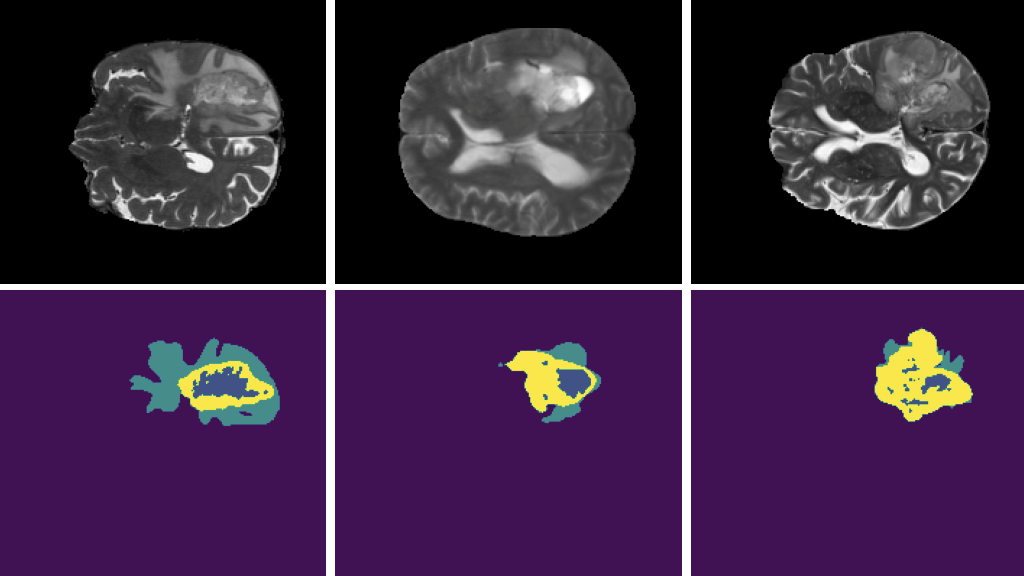\n\nRef: [Accelrating medical image processing with NVIDIA DALI](https://developer.nvidia.com/blog/accelerating-medical-image-processing-with-dali/)\n\n2. Earth Data\n\n -- Before Mask:\n 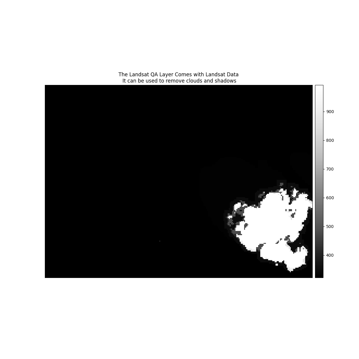 \n -- After Mask:\n 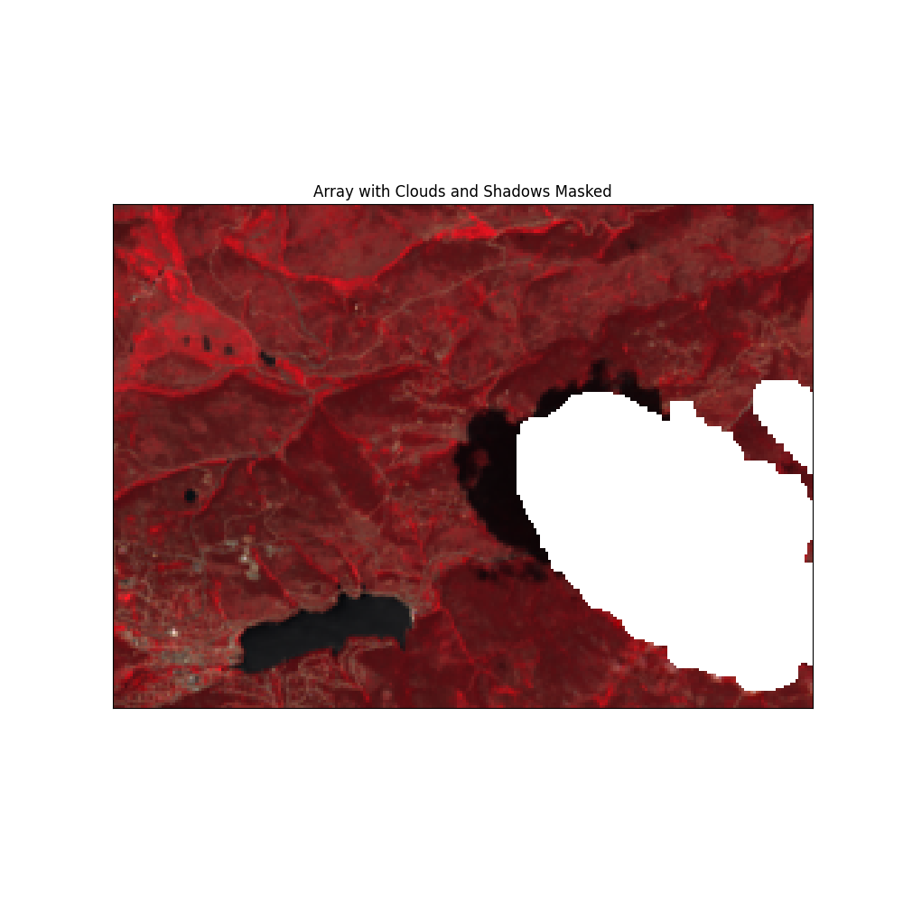\nRef: [Mask and Plot Remote Sensing Data with EarthPy](https://earthpy.readthedocs.io/en/latest/gallery_vignettes/plot_stack_masks.html#mask-and-plot-remote-sensing-data-with-earthpy)\n\n3. Face mask\n\n","metadata":{}},{"cell_type":"markdown","source":"","metadata":{}},{"cell_type":"markdown","source":"> It's time to look at the images and the masks now. The figure below shows randomly selected images corresponding to each of the three distinct cell types. Each cell type has its own unique morphological properties.\n\n* astro instances are the biggest in shape. They cover a lot of space in the masks.\n* cort instances are smaller than the other cell types in general and they are in circle-like shapes. They don't cover much space in the masks.\n* shsy5y instances are slightly bigger, elongated and more abundant than the cort instances. They cover more space than the cort cells.","metadata":{}},{"cell_type":"code","source":"import numpy as np\ndef make_mask(mask_files, image_shape=(520, 704), color=False):\n mask = np.zeros(image_shape).ravel()\n for i, mask_file in enumerate(mask_files):\n couples = np.array(mask_file.split()).reshape(-1, 2).astype(int)\n couples[:, 1] = couples[:, 0] + couples[:, 1]\n for couple in couples:\n if color:\n mask[couple[0]: couple[1]] = i\n else:\n mask[couple[0]: couple[1]] = 1\n mask = mask.reshape(520, 704)\n return mask\n\ndef plot_image(image_id='0030fd0e6378'):\n fig, ax = plt.subplots(1, 2, figsize=(14,5))\n cell_type = df_train.loc[df_train['id'] == image_id, 'cell_type'][0:1].values\n \n file_name = os.path.join(\n '../input/sartorius-cell-instance-segmentation',\n 'train', image_id + '.png')\n image = plt.imread(file_name)\n mask_files = df_train.loc[df_train['id'] == image_id, 'annotation']\n mask = make_mask(mask_files)\n\n ax[0].imshow(\n image,\n cmap = plt.get_cmap('winter'), \n origin = 'upper',\n vmax = np.quantile(image, 0.99),\n vmin = np.quantile(image, 0.05)\n )\n ax[0].set_title(f'Source [{image_id}]')\n ax[0].axis('off')\n \n ax[1].imshow(\n image,\n cmap = plt.get_cmap('winter'), \n origin = 'upper',\n vmax = 255,\n vmin = 0)\n ax[1].imshow(mask, alpha=1, cmap=plt.get_cmap('seismic'))\n ax[1].set_title(f'Source [{image_id}] + Mask {cell_type}')\n ax[1].axis('off')\n plt.show()\n\ndf_train = train_data\n\nselect_image_ids = []\nselect_image_ids.append(df_train.loc[df_train['cell_type'] == 'astro', 'id'].sample(1).to_list()[0])\nselect_image_ids.append(df_train.loc[df_train['cell_type'] == 'cort', 'id'].sample(1).to_list()[0])\nselect_image_ids.append(df_train.loc[df_train['cell_type'] == 'shsy5y', 'id'].sample(1).to_list()[0])\n\nfor image_id in select_image_ids:\n plot_image(image_id)","metadata":{"execution":{"iopub.status.busy":"2022-02-10T12:46:32.956409Z","iopub.execute_input":"2022-02-10T12:46:32.956716Z","iopub.status.idle":"2022-02-10T12:46:33.981114Z","shell.execute_reply.started":"2022-02-10T12:46:32.95667Z","shell.execute_reply":"2022-02-10T12:46:33.98054Z"},"trusted":true},"execution_count":null,"outputs":[]},{"cell_type":"markdown","source":"# Image segmentation with CNN","metadata":{}},{"cell_type":"code","source":"im_ht, im_width, im_channels = 520, 704, 1\n\ntrain_ids = train_data['id'].unique().tolist()\ntest_ids = samplesub['id'].unique().tolist()\n\n\nx_train = np.zeros((train_data['id'].nunique(),im_ht, im_width, im_channels), dtype = np.uint8)\ny_train = np.zeros((train_data['id'].nunique(),im_ht, im_width, im_channels), dtype = np.uint8)\nx_test = np.zeros((samplesub['id'].nunique(),im_ht, im_width, im_channels), dtype = np.uint8)","metadata":{"execution":{"iopub.status.busy":"2022-02-10T12:46:33.981933Z","iopub.execute_input":"2022-02-10T12:46:33.98222Z","iopub.status.idle":"2022-02-10T12:46:34.00248Z","shell.execute_reply.started":"2022-02-10T12:46:33.982196Z","shell.execute_reply":"2022-02-10T12:46:34.001675Z"},"trusted":true},"execution_count":null,"outputs":[]},{"cell_type":"code","source":"from tqdm import tqdm\n\nTRAIN_PATH = '../input/sartorius-cell-instance-segmentation/train/'\n# https://www.kaggle.com/c/sartorius-cell-instance-segmentation/discussion/291627\ndef rle_decode(mask_rle, shape=(520, 704, 1)):\n s = mask_rle.split()\n starts, lengths = [np.asarray(x, dtype=int) for x in (s[0:][::2], s[1:][::2])]\n starts -= 1\n ends = starts + lengths\n img = np.zeros(shape[0]*shape[1], dtype=np.uint8)\n for lo, hi in zip(starts, ends):\n img[lo:hi] = 1\n return img.reshape(shape) # Needed to align to RLE direction\n\ndef rle_encode(img):\n pixels = img.flatten()\n pixels = np.concatenate([[0], pixels, [0]])\n runs = np.where(pixels[1:] != pixels[:-1])[0] + 1\n runs[1::2] -= runs[::2]\n return ' '.join(str(x) for x in runs)\n\nfor n, id_ in tqdm(enumerate(train_ids), total=len(train_ids)):\n path = TRAIN_PATH + id_\n img = cv2.imread(path + '.png')[:,:]\n img = cv2.cvtColor(img, cv2.COLOR_BGR2GRAY).astype(np.float32) -125\n img = np.expand_dims(img, axis = 2)\n x_train[n] = img\n \n labels = train_data[train_data[\"id\"]\n == id_][\"annotation\"].tolist()\n mask = np.zeros((520, 704, 1))\n for label in labels:\n mask += rle_decode(label, shape=(520, 704, 1))\n mask = mask.clip(0, 1)\n\n y_train[n] = mask\nprint(\"Done\")","metadata":{"execution":{"iopub.status.busy":"2022-02-10T12:46:34.003517Z","iopub.execute_input":"2022-02-10T12:46:34.003714Z","iopub.status.idle":"2022-02-10T12:47:17.821736Z","shell.execute_reply.started":"2022-02-10T12:46:34.00369Z","shell.execute_reply":"2022-02-10T12:47:17.820893Z"},"trusted":true},"execution_count":null,"outputs":[]},{"cell_type":"code","source":"# Get and resize test images\ntest_images_id = []\nX_test = np.zeros((samplesub['id'].nunique(), im_ht, im_width, im_channels), dtype=np.uint8)\nfor n, id_ in tqdm(enumerate(test_ids), total=len(test_ids)):\n path = TRAIN_PATH.replace('train', 'test') + id_\n img = cv2.imread(path + '.png')[:,:]\n img = cv2.cvtColor(img, cv2.COLOR_BGR2GRAY).astype(np.float32) -125\n img = np.expand_dims(img, axis = 2)\n X_test[n] = img\n test_images_id.append(id_)\nprint(\"Done\")","metadata":{"execution":{"iopub.status.busy":"2022-02-10T12:47:17.822976Z","iopub.execute_input":"2022-02-10T12:47:17.823212Z","iopub.status.idle":"2022-02-10T12:47:17.866359Z","shell.execute_reply.started":"2022-02-10T12:47:17.823184Z","shell.execute_reply":"2022-02-10T12:47:17.865489Z"},"trusted":true},"execution_count":null,"outputs":[]},{"cell_type":"code","source":"import keras\nfrom keras.models import Model,load_model\nfrom keras import layers\nfrom tensorflow.keras.losses import BinaryCrossentropy\n\nmodel = keras.Sequential([\n keras.layers.Conv2D(filters = 20,kernel_size=5, strides = 1,\n padding = 'same',activation ='relu',\n input_shape = [im_ht, im_width, im_channels]),\n keras.layers.BatchNormalization(),\n keras.layers.Conv2D(filters=10, kernel_size=5, strides = 1,\n padding = 'same',activation ='relu'),\n keras.layers.BatchNormalization(),\n keras.layers.Conv2D(filters=1, kernel_size=1),\n])\n\nmodel.compile(optimizer = 'adam', loss = BinaryCrossentropy(),metrics = ['accuracy'])\nmodel.summary()","metadata":{"execution":{"iopub.status.busy":"2022-02-10T12:47:17.867506Z","iopub.execute_input":"2022-02-10T12:47:17.867723Z","iopub.status.idle":"2022-02-10T12:47:23.296268Z","shell.execute_reply.started":"2022-02-10T12:47:17.867695Z","shell.execute_reply":"2022-02-10T12:47:23.295409Z"},"trusted":true},"execution_count":null,"outputs":[]},{"cell_type":"code","source":"from tensorflow.keras.utils import plot_model\n\nplot_model(model,show_shapes = True)","metadata":{"execution":{"iopub.status.busy":"2022-02-10T12:47:23.297613Z","iopub.execute_input":"2022-02-10T12:47:23.297911Z","iopub.status.idle":"2022-02-10T12:47:24.15433Z","shell.execute_reply.started":"2022-02-10T12:47:23.297872Z","shell.execute_reply":"2022-02-10T12:47:24.152811Z"},"trusted":true},"execution_count":null,"outputs":[]},{"cell_type":"code","source":"from keras.callbacks import EarlyStopping\n# Save the best models and its weights at every step \n\nmodel_output = os.path.join('./','model.h5')\nmodel_checkpoint = keras.callbacks.ModelCheckpoint(\n model_output,save_best_only = True, save_weights_only = True)\n\n# Reduces the learning rate for no model improvement\nlr_reduce = keras.callbacks.ReduceLROnPlateau( monitor='val_loss', factor=0.1, patience=10, verbose=0,\n mode='auto', min_delta=0.0001, cooldown=0, min_lr=0)\n\nes = EarlyStopping(patience = 10, verbose = 1)\n\nhist = model.fit(x_train, y_train, batch_size = 65, \n validation_steps=0.5,\n \n epochs = 5,callbacks = [EarlyStopping(), model_checkpoint, lr_reduce])\n","metadata":{"execution":{"iopub.status.busy":"2022-02-10T12:47:24.156033Z","iopub.execute_input":"2022-02-10T12:47:24.156512Z","iopub.status.idle":"2022-02-10T13:01:49.447057Z","shell.execute_reply.started":"2022-02-10T12:47:24.15647Z","shell.execute_reply":"2022-02-10T13:01:49.446418Z"},"trusted":true},"execution_count":null,"outputs":[]},{"cell_type":"markdown","source":"","metadata":{}},{"cell_type":"code","source":"print(x_train.shape, y_train.shape)\npred = model.predict(x_train)\nprint(pred.shape)\ntrain_preds = (pred > 0.5).astype(np.uint8)\nplt.imshow(train_preds[0],cmap = 'gray')\n","metadata":{"execution":{"iopub.status.busy":"2022-02-10T13:01:49.660321Z","iopub.execute_input":"2022-02-10T13:01:49.660528Z","iopub.status.idle":"2022-02-10T13:02:31.531689Z","shell.execute_reply.started":"2022-02-10T13:01:49.660504Z","shell.execute_reply":"2022-02-10T13:02:31.531045Z"},"trusted":true},"execution_count":null,"outputs":[]},{"cell_type":"code","source":"# Plot model loss\nloss = hist.history['loss']\n\nplt.figure()\nplt.plot(hist.epoch, loss, 'r', label='Training loss')\n\nplt.title('model loss')\nplt.xlabel('epochs')\nplt.ylabel('Loss')\nplt.legend(['loss'],loc = 'right')\nplt.show()","metadata":{"execution":{"iopub.status.busy":"2022-02-10T13:01:49.448424Z","iopub.execute_input":"2022-02-10T13:01:49.44865Z","iopub.status.idle":"2022-02-10T13:01:49.65932Z","shell.execute_reply.started":"2022-02-10T13:01:49.448623Z","shell.execute_reply":"2022-02-10T13:01:49.658471Z"},"trusted":true},"execution_count":null,"outputs":[]},{"cell_type":"code","source":"# Ref: https://www.kaggle.com/carlosgut/sartorius-simple-cnn-keras\npreds_test = model.predict(X_test, verbose=1)\npreds_test_t = (preds_test >= 0.5).astype(np.uint8)\n# Test samples\nfrom random import randint\nix = randint(0, len(preds_test_t)-1)\nprint(ix)\nplt.imshow(X_test[ix])\nplt.show()\nplt.imshow(np.squeeze(preds_test_t[ix]))\nplt.show()","metadata":{"execution":{"iopub.status.busy":"2022-02-10T13:02:31.53302Z","iopub.execute_input":"2022-02-10T13:02:31.533381Z","iopub.status.idle":"2022-02-10T13:02:32.227401Z","shell.execute_reply.started":"2022-02-10T13:02:31.533341Z","shell.execute_reply":"2022-02-10T13:02:32.226632Z"},"trusted":true},"execution_count":null,"outputs":[]},{"cell_type":"markdown","source":"","metadata":{}},{"cell_type":"markdown","source":"If you find this notebook useful, do give me an upvote, it helps to keep up my motivation. This notebook will be updated frequently so keep checking for furthur developments.\n\nCheckout my blog for detailed explanation of this notebook - [Detect single neuronal cells in microscopy images](https://medium.com/@samyukthamantri/detect-single-neuronal-cells-in-microscopy-images-%EF%B8%8F-48b20f072a48)\n\n","metadata":{}},{"cell_type":"markdown","source":"","metadata":{}},{"cell_type":"markdown","source":"","metadata":{}}]}
 ","metadata":{}},{"cell_type":"markdown","source":"# EDA 💟 💟 💟:","metadata":{}},{"cell_type":"markdown","source":" Let's load the data and look at some images in the dataset ","metadata":{}},{"cell_type":"code","source":"import pandas as pd \n\ntrain_data = pd.read_csv('../input/sartorius-cell-instance-segmentation/train.csv')\n\nsamplesub = pd.read_csv('../input/sartorius-cell-instance-segmentation/sample_submission.csv')\nprint('Training set shape',train_data.shape)\ntrain_data.head(5)","metadata":{"execution":{"iopub.status.busy":"2022-02-10T12:46:22.950385Z","iopub.execute_input":"2022-02-10T12:46:22.950724Z","iopub.status.idle":"2022-02-10T12:46:23.516902Z","shell.execute_reply.started":"2022-02-10T12:46:22.950625Z","shell.execute_reply":"2022-02-10T12:46:23.516091Z"},"trusted":true},"execution_count":null,"outputs":[]},{"cell_type":"markdown","source":"### Train dataset information","metadata":{}},{"cell_type":"code","source":"# Train dataset information\n\ntrain_data.info()","metadata":{"_kg_hide-input":true,"execution":{"iopub.status.busy":"2022-02-10T12:46:23.518682Z","iopub.execute_input":"2022-02-10T12:46:23.519496Z","iopub.status.idle":"2022-02-10T12:46:23.565836Z","shell.execute_reply.started":"2022-02-10T12:46:23.519453Z","shell.execute_reply":"2022-02-10T12:46:23.565015Z"},"trusted":true},"execution_count":null,"outputs":[]},{"cell_type":"markdown","source":"### Uniqueness of train data","metadata":{}},{"cell_type":"code","source":"train_data.nunique()","metadata":{"_kg_hide-input":true,"execution":{"iopub.status.busy":"2022-02-10T12:46:23.567268Z","iopub.execute_input":"2022-02-10T12:46:23.567716Z","iopub.status.idle":"2022-02-10T12:46:23.669105Z","shell.execute_reply.started":"2022-02-10T12:46:23.567677Z","shell.execute_reply":"2022-02-10T12:46:23.668222Z"},"trusted":true},"execution_count":null,"outputs":[]},{"cell_type":"markdown","source":"### Different cell types","metadata":{}},{"cell_type":"code","source":"# Different cell types\n\nimport matplotlib.pyplot as plt\n\nfig, ax = plt.subplots(1,1)\ntrain_data.cell_type.value_counts().plot.bar()\nax.set_ylabel('Number of istances')\nax.set_xlabel('Cell types',rotation=0)\nfig.tight_layout()\nplt.show()","metadata":{"_kg_hide-input":true,"execution":{"iopub.status.busy":"2022-02-10T12:46:23.670818Z","iopub.execute_input":"2022-02-10T12:46:23.671045Z","iopub.status.idle":"2022-02-10T12:46:23.832283Z","shell.execute_reply.started":"2022-02-10T12:46:23.671019Z","shell.execute_reply":"2022-02-10T12:46:23.831372Z"},"trusted":true},"execution_count":null,"outputs":[]},{"cell_type":"markdown","source":"The shsy5y is the highest cell type followed by cort cells. Astro is the least occuring cell type.","metadata":{}},{"cell_type":"markdown","source":"### Images in each directory","metadata":{}},{"cell_type":"code","source":"# A class to access parameters and paths for the images\n\nimport tqdm\nimport os\nfrom termcolor import colored\n\nclass config:\n dir = \"../input/sartorius-cell-instance-segmentation\"\n train_path = dir + '/train'\n test_path = dir +'/test'\n\n# A py method to join image dir path and fnames as a list\ndef getImagePath(path):\n image_names = []\n for dirn, _, fnames in os.walk(path):\n for fname in fnames:\n fullpath = os.path.join(dirn, fname)\n #print(fullpath)\n image_names.append(fullpath)\n return image_names\n\ntrain_im_path = getImagePath(config.train_path)\ntest_im_path = getImagePath(config.test_path)\n\nprint('Files in test path \\n',test_im_path[0:5],'\\n') \n\nprint('No. of images in train and test dir\\n',\n 'Train images :',colored(len(train_im_path),'blue'),'\\n'\n 'Test images:',colored(len(test_im_path),'green'))","metadata":{"execution":{"iopub.status.busy":"2022-02-10T12:46:23.833661Z","iopub.execute_input":"2022-02-10T12:46:23.83472Z","iopub.status.idle":"2022-02-10T12:46:24.034399Z","shell.execute_reply.started":"2022-02-10T12:46:23.834677Z","shell.execute_reply":"2022-02-10T12:46:24.033778Z"},"trusted":true},"execution_count":null,"outputs":[]},{"cell_type":"markdown","source":"### Distribution plots","metadata":{}},{"cell_type":"code","source":"import plotly.express as px\ndef dist_plot(x):\n fig = px.histogram(train_data, x = x)\n fig.show()\n\ndist_plot('cell_type')","metadata":{"execution":{"iopub.status.busy":"2022-02-10T12:46:24.035418Z","iopub.execute_input":"2022-02-10T12:46:24.035966Z","iopub.status.idle":"2022-02-10T12:46:26.794811Z","shell.execute_reply.started":"2022-02-10T12:46:24.035933Z","shell.execute_reply":"2022-02-10T12:46:26.794112Z"},"trusted":true},"execution_count":null,"outputs":[]},{"cell_type":"code","source":"dist_plot('plate_time')","metadata":{"execution":{"iopub.status.busy":"2022-02-10T12:46:26.795931Z","iopub.execute_input":"2022-02-10T12:46:26.796233Z","iopub.status.idle":"2022-02-10T12:46:27.360309Z","shell.execute_reply.started":"2022-02-10T12:46:26.796206Z","shell.execute_reply":"2022-02-10T12:46:27.359447Z"},"trusted":true},"execution_count":null,"outputs":[]},{"cell_type":"markdown","source":"Highest Plate time is 11 h","metadata":{}},{"cell_type":"markdown","source":"### Image gallery 🏞🎶\n\n
 \n\nWe will be displaying multiple images in a file directory using computer vision libraries","metadata":{}},{"cell_type":"code","source":"import cv2\ndef im_show(im_paths, r, c):\n fig, ax = plt.subplots(nrows = r, ncols = c, \n figsize = (16,8))\n for p, im_path in enumerate(im_paths):\n im = cv2.imread(im_path)\n im = cv2.cvtColor(im, cv2.COLOR_BGR2RGB)\n try:\n \n ax.ravel()[p].imshow(im)\n ax.ravel()[p].set_axis_off()\n except:\n continue;\n plt.tight_layout()\n plt.show()\n \n","metadata":{"execution":{"iopub.status.busy":"2022-02-10T12:46:27.361346Z","iopub.execute_input":"2022-02-10T12:46:27.361544Z","iopub.status.idle":"2022-02-10T12:46:27.72398Z","shell.execute_reply.started":"2022-02-10T12:46:27.36152Z","shell.execute_reply":"2022-02-10T12:46:27.723281Z"},"trusted":true},"execution_count":null,"outputs":[]},{"cell_type":"code","source":"im_show(train_im_path[0:60],5,5)","metadata":{"execution":{"iopub.status.busy":"2022-02-10T12:46:27.725179Z","iopub.execute_input":"2022-02-10T12:46:27.725395Z","iopub.status.idle":"2022-02-10T12:46:30.777935Z","shell.execute_reply.started":"2022-02-10T12:46:27.725368Z","shell.execute_reply":"2022-02-10T12:46:30.777298Z"},"trusted":true},"execution_count":null,"outputs":[]},{"cell_type":"code","source":"im_show(test_im_path[0:60],5,5)","metadata":{"execution":{"iopub.status.busy":"2022-02-10T12:46:30.779802Z","iopub.execute_input":"2022-02-10T12:46:30.780129Z","iopub.status.idle":"2022-02-10T12:46:32.954719Z","shell.execute_reply.started":"2022-02-10T12:46:30.780102Z","shell.execute_reply":"2022-02-10T12:46:32.95379Z"},"trusted":true},"execution_count":null,"outputs":[]},{"cell_type":"markdown","source":"### Mask plots\n\n* Represent some specific values in a plot\n* Mask ( Hide / Display) specific features present in colormap, dataset, data type { array, list }\n\nEx: \n1. Medical image processing: \n\n\n\nRef: [Accelrating medical image processing with NVIDIA DALI](https://developer.nvidia.com/blog/accelerating-medical-image-processing-with-dali/)\n\n2. Earth Data\n\n -- Before Mask:\n  \n -- After Mask:\n \nRef: [Mask and Plot Remote Sensing Data with EarthPy](https://earthpy.readthedocs.io/en/latest/gallery_vignettes/plot_stack_masks.html#mask-and-plot-remote-sensing-data-with-earthpy)\n\n3. Face mask\n\n","metadata":{}},{"cell_type":"markdown","source":"
\n\nWe will be displaying multiple images in a file directory using computer vision libraries","metadata":{}},{"cell_type":"code","source":"import cv2\ndef im_show(im_paths, r, c):\n fig, ax = plt.subplots(nrows = r, ncols = c, \n figsize = (16,8))\n for p, im_path in enumerate(im_paths):\n im = cv2.imread(im_path)\n im = cv2.cvtColor(im, cv2.COLOR_BGR2RGB)\n try:\n \n ax.ravel()[p].imshow(im)\n ax.ravel()[p].set_axis_off()\n except:\n continue;\n plt.tight_layout()\n plt.show()\n \n","metadata":{"execution":{"iopub.status.busy":"2022-02-10T12:46:27.361346Z","iopub.execute_input":"2022-02-10T12:46:27.361544Z","iopub.status.idle":"2022-02-10T12:46:27.72398Z","shell.execute_reply.started":"2022-02-10T12:46:27.36152Z","shell.execute_reply":"2022-02-10T12:46:27.723281Z"},"trusted":true},"execution_count":null,"outputs":[]},{"cell_type":"code","source":"im_show(train_im_path[0:60],5,5)","metadata":{"execution":{"iopub.status.busy":"2022-02-10T12:46:27.725179Z","iopub.execute_input":"2022-02-10T12:46:27.725395Z","iopub.status.idle":"2022-02-10T12:46:30.777935Z","shell.execute_reply.started":"2022-02-10T12:46:27.725368Z","shell.execute_reply":"2022-02-10T12:46:30.777298Z"},"trusted":true},"execution_count":null,"outputs":[]},{"cell_type":"code","source":"im_show(test_im_path[0:60],5,5)","metadata":{"execution":{"iopub.status.busy":"2022-02-10T12:46:30.779802Z","iopub.execute_input":"2022-02-10T12:46:30.780129Z","iopub.status.idle":"2022-02-10T12:46:32.954719Z","shell.execute_reply.started":"2022-02-10T12:46:30.780102Z","shell.execute_reply":"2022-02-10T12:46:32.95379Z"},"trusted":true},"execution_count":null,"outputs":[]},{"cell_type":"markdown","source":"### Mask plots\n\n* Represent some specific values in a plot\n* Mask ( Hide / Display) specific features present in colormap, dataset, data type { array, list }\n\nEx: \n1. Medical image processing: \n\n\n\nRef: [Accelrating medical image processing with NVIDIA DALI](https://developer.nvidia.com/blog/accelerating-medical-image-processing-with-dali/)\n\n2. Earth Data\n\n -- Before Mask:\n  \n -- After Mask:\n \nRef: [Mask and Plot Remote Sensing Data with EarthPy](https://earthpy.readthedocs.io/en/latest/gallery_vignettes/plot_stack_masks.html#mask-and-plot-remote-sensing-data-with-earthpy)\n\n3. Face mask\n\n","metadata":{}},{"cell_type":"markdown","source":" ","metadata":{}},{"cell_type":"markdown","source":"> It's time to look at the images and the masks now. The figure below shows randomly selected images corresponding to each of the three distinct cell types. Each cell type has its own unique morphological properties.\n\n* astro instances are the biggest in shape. They cover a lot of space in the masks.\n* cort instances are smaller than the other cell types in general and they are in circle-like shapes. They don't cover much space in the masks.\n* shsy5y instances are slightly bigger, elongated and more abundant than the cort instances. They cover more space than the cort cells.","metadata":{}},{"cell_type":"code","source":"import numpy as np\ndef make_mask(mask_files, image_shape=(520, 704), color=False):\n mask = np.zeros(image_shape).ravel()\n for i, mask_file in enumerate(mask_files):\n couples = np.array(mask_file.split()).reshape(-1, 2).astype(int)\n couples[:, 1] = couples[:, 0] + couples[:, 1]\n for couple in couples:\n if color:\n mask[couple[0]: couple[1]] = i\n else:\n mask[couple[0]: couple[1]] = 1\n mask = mask.reshape(520, 704)\n return mask\n\ndef plot_image(image_id='0030fd0e6378'):\n fig, ax = plt.subplots(1, 2, figsize=(14,5))\n cell_type = df_train.loc[df_train['id'] == image_id, 'cell_type'][0:1].values\n \n file_name = os.path.join(\n '../input/sartorius-cell-instance-segmentation',\n 'train', image_id + '.png')\n image = plt.imread(file_name)\n mask_files = df_train.loc[df_train['id'] == image_id, 'annotation']\n mask = make_mask(mask_files)\n\n ax[0].imshow(\n image,\n cmap = plt.get_cmap('winter'), \n origin = 'upper',\n vmax = np.quantile(image, 0.99),\n vmin = np.quantile(image, 0.05)\n )\n ax[0].set_title(f'Source [{image_id}]')\n ax[0].axis('off')\n \n ax[1].imshow(\n image,\n cmap = plt.get_cmap('winter'), \n origin = 'upper',\n vmax = 255,\n vmin = 0)\n ax[1].imshow(mask, alpha=1, cmap=plt.get_cmap('seismic'))\n ax[1].set_title(f'Source [{image_id}] + Mask {cell_type}')\n ax[1].axis('off')\n plt.show()\n\ndf_train = train_data\n\nselect_image_ids = []\nselect_image_ids.append(df_train.loc[df_train['cell_type'] == 'astro', 'id'].sample(1).to_list()[0])\nselect_image_ids.append(df_train.loc[df_train['cell_type'] == 'cort', 'id'].sample(1).to_list()[0])\nselect_image_ids.append(df_train.loc[df_train['cell_type'] == 'shsy5y', 'id'].sample(1).to_list()[0])\n\nfor image_id in select_image_ids:\n plot_image(image_id)","metadata":{"execution":{"iopub.status.busy":"2022-02-10T12:46:32.956409Z","iopub.execute_input":"2022-02-10T12:46:32.956716Z","iopub.status.idle":"2022-02-10T12:46:33.981114Z","shell.execute_reply.started":"2022-02-10T12:46:32.95667Z","shell.execute_reply":"2022-02-10T12:46:33.98054Z"},"trusted":true},"execution_count":null,"outputs":[]},{"cell_type":"markdown","source":"# Image segmentation with CNN","metadata":{}},{"cell_type":"code","source":"im_ht, im_width, im_channels = 520, 704, 1\n\ntrain_ids = train_data['id'].unique().tolist()\ntest_ids = samplesub['id'].unique().tolist()\n\n\nx_train = np.zeros((train_data['id'].nunique(),im_ht, im_width, im_channels), dtype = np.uint8)\ny_train = np.zeros((train_data['id'].nunique(),im_ht, im_width, im_channels), dtype = np.uint8)\nx_test = np.zeros((samplesub['id'].nunique(),im_ht, im_width, im_channels), dtype = np.uint8)","metadata":{"execution":{"iopub.status.busy":"2022-02-10T12:46:33.981933Z","iopub.execute_input":"2022-02-10T12:46:33.98222Z","iopub.status.idle":"2022-02-10T12:46:34.00248Z","shell.execute_reply.started":"2022-02-10T12:46:33.982196Z","shell.execute_reply":"2022-02-10T12:46:34.001675Z"},"trusted":true},"execution_count":null,"outputs":[]},{"cell_type":"code","source":"from tqdm import tqdm\n\nTRAIN_PATH = '../input/sartorius-cell-instance-segmentation/train/'\n# https://www.kaggle.com/c/sartorius-cell-instance-segmentation/discussion/291627\ndef rle_decode(mask_rle, shape=(520, 704, 1)):\n s = mask_rle.split()\n starts, lengths = [np.asarray(x, dtype=int) for x in (s[0:][::2], s[1:][::2])]\n starts -= 1\n ends = starts + lengths\n img = np.zeros(shape[0]*shape[1], dtype=np.uint8)\n for lo, hi in zip(starts, ends):\n img[lo:hi] = 1\n return img.reshape(shape) # Needed to align to RLE direction\n\ndef rle_encode(img):\n pixels = img.flatten()\n pixels = np.concatenate([[0], pixels, [0]])\n runs = np.where(pixels[1:] != pixels[:-1])[0] + 1\n runs[1::2] -= runs[::2]\n return ' '.join(str(x) for x in runs)\n\nfor n, id_ in tqdm(enumerate(train_ids), total=len(train_ids)):\n path = TRAIN_PATH + id_\n img = cv2.imread(path + '.png')[:,:]\n img = cv2.cvtColor(img, cv2.COLOR_BGR2GRAY).astype(np.float32) -125\n img = np.expand_dims(img, axis = 2)\n x_train[n] = img\n \n labels = train_data[train_data[\"id\"]\n == id_][\"annotation\"].tolist()\n mask = np.zeros((520, 704, 1))\n for label in labels:\n mask += rle_decode(label, shape=(520, 704, 1))\n mask = mask.clip(0, 1)\n\n y_train[n] = mask\nprint(\"Done\")","metadata":{"execution":{"iopub.status.busy":"2022-02-10T12:46:34.003517Z","iopub.execute_input":"2022-02-10T12:46:34.003714Z","iopub.status.idle":"2022-02-10T12:47:17.821736Z","shell.execute_reply.started":"2022-02-10T12:46:34.00369Z","shell.execute_reply":"2022-02-10T12:47:17.820893Z"},"trusted":true},"execution_count":null,"outputs":[]},{"cell_type":"code","source":"# Get and resize test images\ntest_images_id = []\nX_test = np.zeros((samplesub['id'].nunique(), im_ht, im_width, im_channels), dtype=np.uint8)\nfor n, id_ in tqdm(enumerate(test_ids), total=len(test_ids)):\n path = TRAIN_PATH.replace('train', 'test') + id_\n img = cv2.imread(path + '.png')[:,:]\n img = cv2.cvtColor(img, cv2.COLOR_BGR2GRAY).astype(np.float32) -125\n img = np.expand_dims(img, axis = 2)\n X_test[n] = img\n test_images_id.append(id_)\nprint(\"Done\")","metadata":{"execution":{"iopub.status.busy":"2022-02-10T12:47:17.822976Z","iopub.execute_input":"2022-02-10T12:47:17.823212Z","iopub.status.idle":"2022-02-10T12:47:17.866359Z","shell.execute_reply.started":"2022-02-10T12:47:17.823184Z","shell.execute_reply":"2022-02-10T12:47:17.865489Z"},"trusted":true},"execution_count":null,"outputs":[]},{"cell_type":"code","source":"import keras\nfrom keras.models import Model,load_model\nfrom keras import layers\nfrom tensorflow.keras.losses import BinaryCrossentropy\n\nmodel = keras.Sequential([\n keras.layers.Conv2D(filters = 20,kernel_size=5, strides = 1,\n padding = 'same',activation ='relu',\n input_shape = [im_ht, im_width, im_channels]),\n keras.layers.BatchNormalization(),\n keras.layers.Conv2D(filters=10, kernel_size=5, strides = 1,\n padding = 'same',activation ='relu'),\n keras.layers.BatchNormalization(),\n keras.layers.Conv2D(filters=1, kernel_size=1),\n])\n\nmodel.compile(optimizer = 'adam', loss = BinaryCrossentropy(),metrics = ['accuracy'])\nmodel.summary()","metadata":{"execution":{"iopub.status.busy":"2022-02-10T12:47:17.867506Z","iopub.execute_input":"2022-02-10T12:47:17.867723Z","iopub.status.idle":"2022-02-10T12:47:23.296268Z","shell.execute_reply.started":"2022-02-10T12:47:17.867695Z","shell.execute_reply":"2022-02-10T12:47:23.295409Z"},"trusted":true},"execution_count":null,"outputs":[]},{"cell_type":"code","source":"from tensorflow.keras.utils import plot_model\n\nplot_model(model,show_shapes = True)","metadata":{"execution":{"iopub.status.busy":"2022-02-10T12:47:23.297613Z","iopub.execute_input":"2022-02-10T12:47:23.297911Z","iopub.status.idle":"2022-02-10T12:47:24.15433Z","shell.execute_reply.started":"2022-02-10T12:47:23.297872Z","shell.execute_reply":"2022-02-10T12:47:24.152811Z"},"trusted":true},"execution_count":null,"outputs":[]},{"cell_type":"code","source":"from keras.callbacks import EarlyStopping\n# Save the best models and its weights at every step \n\nmodel_output = os.path.join('./','model.h5')\nmodel_checkpoint = keras.callbacks.ModelCheckpoint(\n model_output,save_best_only = True, save_weights_only = True)\n\n# Reduces the learning rate for no model improvement\nlr_reduce = keras.callbacks.ReduceLROnPlateau( monitor='val_loss', factor=0.1, patience=10, verbose=0,\n mode='auto', min_delta=0.0001, cooldown=0, min_lr=0)\n\nes = EarlyStopping(patience = 10, verbose = 1)\n\nhist = model.fit(x_train, y_train, batch_size = 65, \n validation_steps=0.5,\n \n epochs = 5,callbacks = [EarlyStopping(), model_checkpoint, lr_reduce])\n","metadata":{"execution":{"iopub.status.busy":"2022-02-10T12:47:24.156033Z","iopub.execute_input":"2022-02-10T12:47:24.156512Z","iopub.status.idle":"2022-02-10T13:01:49.447057Z","shell.execute_reply.started":"2022-02-10T12:47:24.15647Z","shell.execute_reply":"2022-02-10T13:01:49.446418Z"},"trusted":true},"execution_count":null,"outputs":[]},{"cell_type":"markdown","source":"
 ","metadata":{}},{"cell_type":"code","source":"print(x_train.shape, y_train.shape)\npred = model.predict(x_train)\nprint(pred.shape)\ntrain_preds = (pred > 0.5).astype(np.uint8)\nplt.imshow(train_preds[0],cmap = 'gray')\n","metadata":{"execution":{"iopub.status.busy":"2022-02-10T13:01:49.660321Z","iopub.execute_input":"2022-02-10T13:01:49.660528Z","iopub.status.idle":"2022-02-10T13:02:31.531689Z","shell.execute_reply.started":"2022-02-10T13:01:49.660504Z","shell.execute_reply":"2022-02-10T13:02:31.531045Z"},"trusted":true},"execution_count":null,"outputs":[]},{"cell_type":"code","source":"# Plot model loss\nloss = hist.history['loss']\n\nplt.figure()\nplt.plot(hist.epoch, loss, 'r', label='Training loss')\n\nplt.title('model loss')\nplt.xlabel('epochs')\nplt.ylabel('Loss')\nplt.legend(['loss'],loc = 'right')\nplt.show()","metadata":{"execution":{"iopub.status.busy":"2022-02-10T13:01:49.448424Z","iopub.execute_input":"2022-02-10T13:01:49.44865Z","iopub.status.idle":"2022-02-10T13:01:49.65932Z","shell.execute_reply.started":"2022-02-10T13:01:49.448623Z","shell.execute_reply":"2022-02-10T13:01:49.658471Z"},"trusted":true},"execution_count":null,"outputs":[]},{"cell_type":"code","source":"# Ref: https://www.kaggle.com/carlosgut/sartorius-simple-cnn-keras\npreds_test = model.predict(X_test, verbose=1)\npreds_test_t = (preds_test >= 0.5).astype(np.uint8)\n# Test samples\nfrom random import randint\nix = randint(0, len(preds_test_t)-1)\nprint(ix)\nplt.imshow(X_test[ix])\nplt.show()\nplt.imshow(np.squeeze(preds_test_t[ix]))\nplt.show()","metadata":{"execution":{"iopub.status.busy":"2022-02-10T13:02:31.53302Z","iopub.execute_input":"2022-02-10T13:02:31.533381Z","iopub.status.idle":"2022-02-10T13:02:32.227401Z","shell.execute_reply.started":"2022-02-10T13:02:31.533341Z","shell.execute_reply":"2022-02-10T13:02:32.226632Z"},"trusted":true},"execution_count":null,"outputs":[]},{"cell_type":"markdown","source":"
 ","metadata":{}},{"cell_type":"markdown","source":"If you find this notebook useful, do give me an upvote, it helps to keep up my motivation. This notebook will be updated frequently so keep checking for furthur developments.\n\nCheckout my blog for detailed explanation of this notebook - [Detect single neuronal cells in microscopy images](https://medium.com/@samyukthamantri/detect-single-neuronal-cells-in-microscopy-images-%EF%B8%8F-48b20f072a48)\n\n
 ","metadata":{}},{"cell_type":"markdown","source":"","metadata":{}},{"cell_type":"markdown","source":"","metadata":{}}]}