{"metadata":{"kernelspec":{"language":"python","display_name":"Python 3","name":"python3"},"language_info":{"pygments_lexer":"ipython3","nbconvert_exporter":"python","version":"3.6.4","file_extension":".py","codemirror_mode":{"name":"ipython","version":3},"name":"python","mimetype":"text/x-python"}},"nbformat_minor":4,"nbformat":4,"cells":[{"cell_type":"code","source":"import os\nimport tensorflow as tf\nimport numpy as np\nimport matplotlib.pyplot as plt\nimport pandas as pd\nimport cv2\nimport tensorflow.keras.backend as K\nfrom sklearn.model_selection import train_test_split\nfrom IPython.display import clear_output\n\n\nimport warnings\n\nwarnings.filterwarnings(\"ignore\")","metadata":{"execution":{"iopub.status.busy":"2021-12-25T13:37:49.543010Z","iopub.execute_input":"2021-12-25T13:37:49.543378Z","iopub.status.idle":"2021-12-25T13:37:56.011878Z","shell.execute_reply.started":"2021-12-25T13:37:49.543261Z","shell.execute_reply":"2021-12-25T13:37:56.010832Z"},"trusted":true},"execution_count":null,"outputs":[]},{"cell_type":"markdown","source":"# Sartorius Competition \n\n**Overview**\n\nIn Sartorius Cell Instance Segmentation challenge we are faced with a task to perform instance segmentation on medical images to find neuronal cells. Successful segmentation could lead to the discovery of new drugs and treatments for neurodegenerative diseases such as Alzimer's and brain tumors.\n\n**Data**\n\ntrain.csv file provided to competitors contains the following columns \n- id - unique identifier\n- annotation - run length encoded pixels for the identified neuronal cell\n- width - image width\n- height - image height\n- cell_type - class of the cell\n- plate_time - time the plate was created\n- sample_id - id of the sample\n- sample_date - date the sample was created\n- elapsed_timedelta - time since the image was shot\n\n\nids present in the column id correspond to image files in train folder\n\nannotations are run length encoded pixels in order to create a mask we will have to decode the annotations","metadata":{}},{"cell_type":"code","source":"class Config:\n '''\n Config in which I hold all hyperparameters and frequently used variables such as image shape, train directory path etc.\n '''\n def __init__(self, DEBUG=False):\n self.DEBUG = DEBUG\n \n TRAIN_CSV = '../input/sartorius-cell-instance-segmentation/train.csv'\n TRAIN_DIR = '../input/sartorius-cell-instance-segmentation/train/'\n TEST_DIR = '../input/sartorius-cell-instance-segmentation/test/'\n \n IMG_SHAPE = (512, 512)\n \n LR = 1e-3\n \n EPOCHS = 100\n \n N_FILTERS = 32\n\n \n BATCH_SIZE = 4\n AUTOTUNE = tf.data.AUTOTUNE\n \n N_CLASSES = 1\n BUFFER_SIZE = 2\n \n val_size = 0.1\n \n WEIGHTS_PATH = os.path.join('./', 'model.h5')\n \n seed = 123\n \n\nconfig = Config()","metadata":{"execution":{"iopub.status.busy":"2021-12-25T13:37:56.015968Z","iopub.execute_input":"2021-12-25T13:37:56.016222Z","iopub.status.idle":"2021-12-25T13:37:56.029129Z","shell.execute_reply.started":"2021-12-25T13:37:56.016192Z","shell.execute_reply":"2021-12-25T13:37:56.027392Z"},"trusted":true},"execution_count":null,"outputs":[]},{"cell_type":"markdown","source":"# Data Loading And Exploration\n\nFirst lets load train.csv to pandas dataframe and take a look at out data","metadata":{}},{"cell_type":"code","source":"train_csv = pd.read_csv(Config.TRAIN_CSV)\ntrain_csv.head()","metadata":{"execution":{"iopub.status.busy":"2021-12-25T13:37:56.033564Z","iopub.execute_input":"2021-12-25T13:37:56.033834Z","iopub.status.idle":"2021-12-25T13:37:56.742708Z","shell.execute_reply.started":"2021-12-25T13:37:56.033793Z","shell.execute_reply":"2021-12-25T13:37:56.741510Z"},"trusted":true},"execution_count":null,"outputs":[]},{"cell_type":"markdown","source":"First thing I've noticed is that the same ID appears several times with different annotations, it means that each annotation is only for one cell, and that the annotations might overlap \n\n**Let's take a look at a single image**","metadata":{}},{"cell_type":"code","source":"plt.figure(figsize=(15,15))\n\nplt.imshow(cv2.imread(config.TRAIN_DIR + '0030fd0e6378' + '.png'))\nplt.axis(\"off\")\nplt.show()","metadata":{"execution":{"iopub.status.busy":"2021-12-25T13:37:56.745591Z","iopub.execute_input":"2021-12-25T13:37:56.745992Z","iopub.status.idle":"2021-12-25T13:37:57.229304Z","shell.execute_reply.started":"2021-12-25T13:37:56.745948Z","shell.execute_reply":"2021-12-25T13:37:57.228493Z"},"trusted":true},"execution_count":null,"outputs":[]},{"cell_type":"markdown","source":"Knowing that ids might appear several times let's see how large our dataset is","metadata":{}},{"cell_type":"code","source":"train_csv.shape","metadata":{"execution":{"iopub.status.busy":"2021-12-25T13:37:57.230412Z","iopub.execute_input":"2021-12-25T13:37:57.230695Z","iopub.status.idle":"2021-12-25T13:37:57.239043Z","shell.execute_reply.started":"2021-12-25T13:37:57.230658Z","shell.execute_reply":"2021-12-25T13:37:57.237938Z"},"trusted":true},"execution_count":null,"outputs":[]},{"cell_type":"markdown","source":"But how large is it when we take into the account that id is unique?","metadata":{}},{"cell_type":"code","source":"train_csv[\"id\"].unique().shape","metadata":{"execution":{"iopub.status.busy":"2021-12-25T13:37:57.240737Z","iopub.execute_input":"2021-12-25T13:37:57.241411Z","iopub.status.idle":"2021-12-25T13:37:57.266360Z","shell.execute_reply.started":"2021-12-25T13:37:57.241357Z","shell.execute_reply":"2021-12-25T13:37:57.265246Z"},"trusted":true},"execution_count":null,"outputs":[]},{"cell_type":"markdown","source":"Let's see how our dataframe looks for a single id","metadata":{}},{"cell_type":"code","source":"train_csv[train_csv['id'] == '0030fd0e6378']","metadata":{"execution":{"iopub.status.busy":"2021-12-25T13:37:57.268272Z","iopub.execute_input":"2021-12-25T13:37:57.268834Z","iopub.status.idle":"2021-12-25T13:37:57.307360Z","shell.execute_reply.started":"2021-12-25T13:37:57.268791Z","shell.execute_reply":"2021-12-25T13:37:57.306498Z"},"trusted":true},"execution_count":null,"outputs":[]},{"cell_type":"markdown","source":"# Load Data\n\nMasks are encoded in the annotation column by an algorithm called **Run Length Encoding**. RLE encodes a mask into a vector where vector index corresponds to flattened mask matrix index and the value at that index corresponds to length of the annotation, for a more in depth understanding I recommend looking into [this](https://www.kaggle.com/ihelon/cell-segmentation-run-length-decoding) notebook","metadata":{}},{"cell_type":"code","source":"def rle_decode(mask_rle, shape, color=1):\n '''\n mask_rle: run-length as string formated (start length)\n shape: (height,width) of array to return \n Returns numpy array, 1 - mask, 0 - background\n\n '''\n s = mask_rle.split()\n starts, lengths = [np.asarray(x, dtype=int) for x in (s[0:][::2], s[1:][::2])]\n starts -= 1\n ends = starts + lengths\n img = np.zeros((shape[0] * shape[1], shape[2]), dtype=np.float32)\n for lo, hi in zip(starts, ends):\n img[lo : hi] = color\n return img.reshape(shape)\n\n\ndef build_masks(labels, input_shape, colors=True):\n height, width = input_shape\n if colors:\n mask = np.zeros((height, width, 3))\n for label in labels:\n mask += rle_decode(label, shape=(height, width , 3), color=np.random.rand(3))\n else:\n mask = np.zeros((height, width, 1))\n for label in labels:\n mask += rle_decode(label, shape=(height, width, 1))\n mask = mask.clip(0, 1)\n return mask","metadata":{"execution":{"iopub.status.busy":"2021-12-25T13:37:57.308855Z","iopub.execute_input":"2021-12-25T13:37:57.309166Z","iopub.status.idle":"2021-12-25T13:37:57.320523Z","shell.execute_reply.started":"2021-12-25T13:37:57.309129Z","shell.execute_reply":"2021-12-25T13:37:57.319219Z"},"trusted":true},"execution_count":null,"outputs":[]},{"cell_type":"markdown","source":"# Data Vizualization\n\nNow knowing how to load our data we can finally see how the annotations for neuronal cells look like\n\nLet's see how many classes there are for the cell_type column and what the distribution looks like","metadata":{}},{"cell_type":"code","source":"train_csv[\"cell_type\"].unique()","metadata":{"execution":{"iopub.status.busy":"2021-12-25T13:37:57.322660Z","iopub.execute_input":"2021-12-25T13:37:57.322990Z","iopub.status.idle":"2021-12-25T13:37:57.343517Z","shell.execute_reply.started":"2021-12-25T13:37:57.322948Z","shell.execute_reply":"2021-12-25T13:37:57.342300Z"},"trusted":true},"execution_count":null,"outputs":[]},{"cell_type":"code","source":"cell_types = train_csv[\"cell_type\"].value_counts()\n\nplt.figure(figsize=(10, 6), tight_layout=True)\n\nplt.bar(cell_types.index, cell_types.values)\nplt.show()","metadata":{"execution":{"iopub.status.busy":"2021-12-25T13:37:57.348671Z","iopub.execute_input":"2021-12-25T13:37:57.348961Z","iopub.status.idle":"2021-12-25T13:37:57.592641Z","shell.execute_reply.started":"2021-12-25T13:37:57.348930Z","shell.execute_reply":"2021-12-25T13:37:57.591441Z"},"trusted":true},"execution_count":null,"outputs":[]},{"cell_type":"markdown","source":"The distribution is clearly skewed, **shsy5y** cell images domminate the dataset, this might cause our model to have worse performance on other cell types\n\nData augmentation should be performed on the dataset in order to fight this issue","metadata":{}},{"cell_type":"code","source":"shy5y_sample = train_csv[train_csv['cell_type'] == 'shsy5y'].sample(2)['id']\ncort_sample = train_csv[train_csv['cell_type'] == 'cort'].sample(2)['id']\nastro_sample = train_csv[train_csv['cell_type'] == 'astro'].sample(2)['id']","metadata":{"execution":{"iopub.status.busy":"2021-12-25T13:37:57.594312Z","iopub.execute_input":"2021-12-25T13:37:57.594688Z","iopub.status.idle":"2021-12-25T13:37:57.643481Z","shell.execute_reply.started":"2021-12-25T13:37:57.594644Z","shell.execute_reply":"2021-12-25T13:37:57.642571Z"},"trusted":true},"execution_count":null,"outputs":[]},{"cell_type":"markdown","source":"**Let's see how the annotations look like**","metadata":{}},{"cell_type":"code","source":"def display_sample(sample_ids, n_samples=2, hspace=-0.6):\n '''\n Function to visualize images and their annotations\n \n sample_ids - list of ids\n n_samples - number of samples to display\n hspace - parameter for matplotlib, it contorls spacing between images \n '''\n fig, axs = plt.subplots(n_samples, 3, figsize=(22, 25))\n \n for idx, sample_id in enumerate(sample_ids):\n sample_image = cv2.imread(os.path.join(config.TRAIN_DIR + sample_id + '.png'))\n \n sample_rles = train_csv.loc[train_csv['id'] == sample_id]['annotation'].values\n \n sample_mask_colors = build_masks(sample_rles, (520, 704), colors=True)\n sample_mask = build_masks(sample_rles, (520, 704), colors=False)\n \n axs[idx][0].imshow(sample_image)\n axs[idx][0].axis('off') \n \n axs[idx][1].imshow(sample_mask_colors) \n axs[idx][1].axis('off') \n \n axs[idx][2].imshow(sample_mask)\n axs[idx][2].axis('off') \n\n axs[0][0].set_title(\"Image\", fontsize=16)\n axs[0][1].set_title(\"Mask Color\", fontsize=16)\n axs[0][2].set_title(\"Mask\", fontsize=16)\n\n fig.subplots_adjust(hspace=hspace)\n plt.show() ","metadata":{"execution":{"iopub.status.busy":"2021-12-25T13:37:57.644954Z","iopub.execute_input":"2021-12-25T13:37:57.645327Z","iopub.status.idle":"2021-12-25T13:37:57.657365Z","shell.execute_reply.started":"2021-12-25T13:37:57.645281Z","shell.execute_reply":"2021-12-25T13:37:57.655872Z"},"trusted":true},"execution_count":null,"outputs":[]},{"cell_type":"markdown","source":"**SHY5Y**","metadata":{}},{"cell_type":"code","source":"display_sample(shy5y_sample)","metadata":{"execution":{"iopub.status.busy":"2021-12-25T13:37:57.659806Z","iopub.execute_input":"2021-12-25T13:37:57.660407Z","iopub.status.idle":"2021-12-25T13:38:00.442487Z","shell.execute_reply.started":"2021-12-25T13:37:57.660306Z","shell.execute_reply":"2021-12-25T13:38:00.438577Z"},"trusted":true},"execution_count":null,"outputs":[]},{"cell_type":"markdown","source":"**CORT**","metadata":{}},{"cell_type":"code","source":"display_sample(cort_sample)","metadata":{"execution":{"iopub.status.busy":"2021-12-25T13:38:00.444751Z","iopub.execute_input":"2021-12-25T13:38:00.445177Z","iopub.status.idle":"2021-12-25T13:38:01.601043Z","shell.execute_reply.started":"2021-12-25T13:38:00.445135Z","shell.execute_reply":"2021-12-25T13:38:01.596816Z"},"trusted":true},"execution_count":null,"outputs":[]},{"cell_type":"markdown","source":"**ASTRO**","metadata":{}},{"cell_type":"code","source":"display_sample(astro_sample)","metadata":{"execution":{"iopub.status.busy":"2021-12-25T13:38:01.602899Z","iopub.execute_input":"2021-12-25T13:38:01.603465Z","iopub.status.idle":"2021-12-25T13:38:02.998373Z","shell.execute_reply.started":"2021-12-25T13:38:01.603423Z","shell.execute_reply":"2021-12-25T13:38:02.997509Z"},"trusted":true},"execution_count":null,"outputs":[]},{"cell_type":"markdown","source":"# Preparing training and validation datasets\n\nIn order to train the neural network we have to load the data and optimize it for training\n\nfirst train dataset has to be split into training and validation parts\n\n**Validation dataset** is used to validate how well your model is doing before performing predictions on test dataset. Having a validation dataset helps to detect wheter the model is overtrained","metadata":{}},{"cell_type":"code","source":"ids = train_csv['id'].unique()\n\ntrain_ids, val_ids = train_test_split(ids, test_size=config.val_size, random_state=config.seed)","metadata":{"execution":{"iopub.status.busy":"2021-12-25T13:38:02.999621Z","iopub.execute_input":"2021-12-25T13:38:03.000011Z","iopub.status.idle":"2021-12-25T13:38:03.016731Z","shell.execute_reply.started":"2021-12-25T13:38:02.999974Z","shell.execute_reply":"2021-12-25T13:38:03.015499Z"},"trusted":true},"execution_count":null,"outputs":[]},{"cell_type":"code","source":"train_ids.shape","metadata":{"execution":{"iopub.status.busy":"2021-12-25T13:38:03.018541Z","iopub.execute_input":"2021-12-25T13:38:03.020186Z","iopub.status.idle":"2021-12-25T13:38:03.028169Z","shell.execute_reply.started":"2021-12-25T13:38:03.020138Z","shell.execute_reply":"2021-12-25T13:38:03.026843Z"},"trusted":true},"execution_count":null,"outputs":[]},{"cell_type":"markdown","source":"Tensorflow provides tf.data.Dataset api which is very usefull when creating data pipelines for ML models, since it supports caching, batching, one can perform data preprocessing using .map method on Dataset object.\n\nTensorflow docs - https://www.tensorflow.org/guide/data","metadata":{}},{"cell_type":"code","source":"def load_train_ds():\n '''\n This function creates a generator for train dataset\n '''\n for image_id in train_ids:\n rows = train_csv.loc[train_csv['id'] == image_id]\n image = tf.io.read_file(config.TRAIN_DIR + image_id + '.png')\n image = tf.image.decode_image(image, channels=3, dtype=tf.float32)\n rles = rows['annotation'].values\n\n mask = build_masks(rles, (520, 704), colors=False)\n mask = tf.cast(tf.image.resize(mask, config.IMG_SHAPE), tf.int32)\n\n image = tf.image.resize(image, config.IMG_SHAPE)\n image /= 255.0\n \n yield image, mask\n \n \ndef load_val_ds():\n '''\n This function creates a generator for train dataset\n '''\n for image_id in val_ids:\n rows = train_csv.loc[train_csv['id'] == image_id]\n image = tf.io.read_file(config.TRAIN_DIR + image_id + '.png')\n image = tf.image.decode_image(image, channels=3, dtype=tf.float32)\n rles = rows['annotation'].values\n\n mask = build_masks(rles, (520, 704), colors=False)\n mask = tf.cast(tf.image.resize(mask, config.IMG_SHAPE), tf.int32)\n\n image = tf.image.resize(image, config.IMG_SHAPE)\n image /= 255.0\n \n yield image, mask","metadata":{"execution":{"iopub.status.busy":"2021-12-25T13:38:03.030607Z","iopub.execute_input":"2021-12-25T13:38:03.031437Z","iopub.status.idle":"2021-12-25T13:38:03.046795Z","shell.execute_reply.started":"2021-12-25T13:38:03.031302Z","shell.execute_reply":"2021-12-25T13:38:03.045514Z"},"trusted":true},"execution_count":null,"outputs":[]},{"cell_type":"markdown","source":"Having created functions that yield images and masks we can use from_generator method to create datasets from generators","metadata":{}},{"cell_type":"code","source":"train_ds = tf.data.Dataset.from_generator(\n load_train_ds, \n output_types=(tf.float32, tf.int32)\n)\n\nval_ds = tf.data.Dataset.from_generator(\n load_val_ds, \n output_types=(tf.float32, tf.int32)\n)","metadata":{"execution":{"iopub.status.busy":"2021-12-25T13:38:03.049996Z","iopub.execute_input":"2021-12-25T13:38:03.050571Z","iopub.status.idle":"2021-12-25T13:38:05.811038Z","shell.execute_reply.started":"2021-12-25T13:38:03.050524Z","shell.execute_reply":"2021-12-25T13:38:05.810102Z"},"trusted":true},"execution_count":null,"outputs":[]},{"cell_type":"markdown","source":"As I've mentioned before the dataset is severly inbalanced which can cause our model to perform worse in some cases. One popular and simple method to fight this problem is **data augmentation**.\n\n**Data Augmentation** is a method to artifically expand dataset by slightly modifing existing data in a realistic way, for my case I will flip the images horizontally and vertically\n\nTensorflow docs - https://www.tensorflow.org/tutorials/images/data_augmentation","metadata":{}},{"cell_type":"code","source":"def augment_ds(image, mask):\n image = tf.image.random_flip_up_down(image, seed=config.seed)\n mask = tf.image.random_flip_up_down(mask, seed=config.seed)\n \n image = tf.image.random_flip_left_right(image, seed=config.seed)\n mask = tf.image.random_flip_left_right(mask, seed=config.seed)\n \n return image, mask","metadata":{"execution":{"iopub.status.busy":"2021-12-25T13:38:05.812394Z","iopub.execute_input":"2021-12-25T13:38:05.812958Z","iopub.status.idle":"2021-12-25T13:38:05.820942Z","shell.execute_reply.started":"2021-12-25T13:38:05.812899Z","shell.execute_reply":"2021-12-25T13:38:05.819824Z"},"trusted":true},"execution_count":null,"outputs":[]},{"cell_type":"code","source":"train_ds = (\n train_ds\n .shuffle(config.BUFFER_SIZE)\n .map(augment_ds)\n .batch(config.BATCH_SIZE) \n .prefetch(Config.AUTOTUNE)\n)\n\nval_ds = val_ds.batch(config.BATCH_SIZE)","metadata":{"execution":{"iopub.status.busy":"2021-12-25T13:38:05.822776Z","iopub.execute_input":"2021-12-25T13:38:05.823491Z","iopub.status.idle":"2021-12-25T13:38:06.148663Z","shell.execute_reply.started":"2021-12-25T13:38:05.823446Z","shell.execute_reply":"2021-12-25T13:38:06.147455Z"},"trusted":true},"execution_count":null,"outputs":[]},{"cell_type":"code","source":"sample_batch = next(iter(train_ds))\n\nimages, masks = sample_batch\n\nfig, ax = plt.subplots(config.BATCH_SIZE, 2, figsize=(20, 20))\n\nfor i in range(config.BATCH_SIZE):\n ax[i][0].imshow(images[i] * 255)\n ax[i][0].axis('off') \n \n ax[i][1].imshow(masks[i]) \n ax[i][1].axis('off') \n\nplt.show()","metadata":{"execution":{"iopub.status.busy":"2021-12-25T13:38:06.151532Z","iopub.execute_input":"2021-12-25T13:38:06.152441Z","iopub.status.idle":"2021-12-25T13:38:08.128340Z","shell.execute_reply.started":"2021-12-25T13:38:06.152392Z","shell.execute_reply":"2021-12-25T13:38:08.127498Z"},"trusted":true},"execution_count":null,"outputs":[]},{"cell_type":"markdown","source":"# Modeling\n\n**UNET** is a Conv net architecture proposed by Olaf Ronneberger, Philipp Fischer, Thomas Brox in their paper [U-Net: Convolutional Networks for Biomedical Image Segmentation\n](https://arxiv.org/pdf/1505.04597.pdf). It has been very successful in performing semantic segmantation on many benchmarks. The architecture is composed by encoder and decoder networks with a bottleneck in between. Let's see a visualization from the authors.\n\n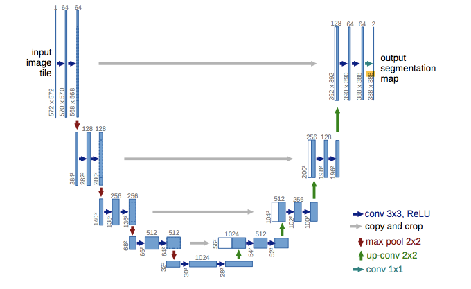 \n\n**The encoder** is composed of conv block each with two 3x3 conv layers followed by max pooling with pool size of 2, there is a total of 4 of this layers with number of filters 512, 256, 128, 64\n\n**The bottlenck** is a simple conv block of two 3x3 conv layers with 1024 filters\n\n**The decoder** consists of 4 upsampling conv block, each having tranposed conv layers with filters size of 2 and strides of 2, after upsampling skip connections are added, lastly two conv 3x3 layers are applied\n\nKey idea of UNET are **skip connections**. Output of each encoder layer is added to corresponding decoder layer, this preserves the spatial structure of the input image, since upsampling in the decoder leaves unprecise expansions. Adding output from encoder layer helps with preserving a lot of information.\n\n# Residual UNET \n**Residual UNET** simply is a UNET with residual conv blocks instead of regular conv blocks, the architecture looks like this\n\n
 \n\nIt was proposed by Zhengxin Zhang, Qingjie Liu, Yunhong Wang in their paper [Road Extraction by Deep Residual U-Net](https://arxiv.org/abs/1711.10684).\n
\n**What are residual conv blocks?** First let's see a simple visualization of a residual unit\n\n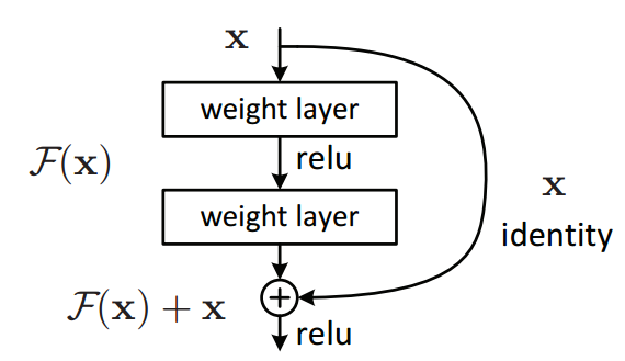 \n\nIn normal conv units tensors are directly propagated throught conv layers. This way of propagation has one big issue - **vanishing gradients**. Vanishing gradients problem occurs when training very deep networks, during backpropagation gradinets are propagated from deeper layers into shallower ones, sometimes the gradients can get smaller (close to 0) at each consecutive layer, this prevents the network from learning. Residual units first save input tensor then propagate them throught conv layers, then add saved input tensor to conv layers output, thus learning **identity mapping** and greatly helping with the vanishing gradients problem.\n\n# Residual UNET with Attention\nAttention was introduced to UNET in 2018's paper [Attention U-Net: Learning Where to Look for the Pancreas](https://arxiv.org/pdf/1804.03999) by Ozan Oktay et al.\n\n**What is attention in the context of computer vision?** Attention is very often used in NLP problems as a way to make a model focus more on for example a part of a sentence. In computer vision attention is a mechanism that allows your network to look only at certain parts of image. Such a part is called a **region of interest** (ROI). Looking at only parts of an image increases computational efficiency, while adding only a small amount of parameters. Below is a diagram from the paper, as you can see attention gate is aplied before concatenation skip connetions to decoder layer.\n\n
 \n\n**Why is attention needed for UNET?** Skip connections are main characteristic of UNET, they help to preserve spatial structure in the upsampling layers. One issue with skip connections is that since they come from shallower layers of the network they extract less complex feature maps, this means that many unuseful low-level features are concatenated to the decoder, attention learns which of those features are worth taking a look at and which are just noise. The end result is a more computationaly efficient network and slighlty better performance. Let's break down the attention gate architecutre. \n\n
 \n\nAttention gate takes as a input a skip connection and the output from the previous decoder layer. Matematically attention gate does the following operation\n\n$$ q_{att}^{l} = \\upsilon^{T}(\\sigma_1(W^{T}_{x}x^{l}_{i} + W^{T}_{g}g_{i} + b_{g})) + b_{\\upsilon} $$\n$$ \\alpha_{i}^{l} = \\sigma_{2}(q_{att}^{l}(x_{i}^{l}, g_{i}; \\Theta_{att})) $$\n\nWhere $\\sigma_{2}(x_{i,c}) = \\frac{1}{1+\\exp(-x_{i, c})}$, $\\Theta_{att}$ contains linear transformations $W_x, W_g$, which are computed using 1x1x1 convolutions for the input tensors. Let's see how we can implement this.\n\n* Input g (previous decoder layer output) and x (skip connection)\n* Convolve x with 1x1 filter and stride = 2, and g with 1x1 filter and stride = 1\n* Add together x and g\n* Apply ReLU activation function\n* $\\psi =$ 1x1x1 convolution \n* Apply sigmoid activation function\n* Upsample sigmoid output to original input size (2x2)\n* $att = multiply(upsample, x_{input})$ \n* 1x1 convolution with n_filters = n_input_x_filters and batch normalization","metadata":{}},{"cell_type":"code","source":"def attention(input_tensor, g, inter_shape): \n input_shapes = input_tensor.shape\n g_shapes = g.shape\n \n x = tf.keras.layers.Conv2D(inter_shape, 1, 2, padding=\"same\")(input_tensor)\n g = tf.keras.layers.Conv2D(inter_shape, 1, padding=\"same\")(g)\n\n\n add = tf.keras.layers.add([x, g])\n relu = tf.keras.layers.Activation('relu')(x)\n \n psi = tf.keras.layers.Conv2D(1, 1, padding=\"same\")(relu)\n sigmoid = tf.keras.layers.Activation('sigmoid')(psi)\n \n upsample = tf.keras.layers.UpSampling2D(size=(2, 2))(sigmoid)\n \n att = tf.keras.layers.multiply([upsample, input_tensor])\n \n output = tf.keras.layers.Conv2D(input_shapes[3], 1, padding=\"same\")(att)\n return tf.keras.layers.BatchNormalization()(output)\n\ndef conv_block(input_tensor, n_filters, dropout=0.5, batch_norm=True):\n x_save = tf.keras.layers.Conv2D(n_filters, 3, activation=\"relu\", padding=\"same\")(input_tensor)\n if batch_norm:\n x = tf.keras.layers.BatchNormalization()(x_save)\n \n x = tf.keras.layers.Conv2D(n_filters, 3, activation=\"relu\", padding=\"same\")(x)\n if batch_norm:\n x = tf.keras.layers.BatchNormalization()(x)\n \n if dropout:\n x = tf.keras.layers.Dropout(dropout)(x)\n \n x = tf.keras.layers.add([x, x_save])\n x = tf.keras.layers.Activation(\"relu\")(x)\n\n return x\n\ndef downsample(x, n_filters, dropout=0.5, batch_norm=True):\n res_conn = conv_block(x, n_filters, dropout=dropout, batch_norm=batch_norm)\n \n x = tf.keras.layers.MaxPool2D((2, 2), strides=(2, 2))(res_conn)\n \n return x, res_conn\n\ndef upsample(x, n_filters, skip_conn, dropout=0.5, batch_norm=True):\n att = attention(skip_conn, x, n_filters)\n x = tf.keras.layers.Conv2DTranspose(n_filters, (2, 2), strides=2, padding=\"same\", activation=\"relu\")(x)\n x = tf.keras.layers.Concatenate()([x, att])\n x = conv_block(x, n_filters)\n \n if dropout:\n x = tf.keras.layers.Dropout(dropout)(x)\n\n if batch_norm:\n x = tf.keras.layers.BatchNormalization()(x)\n \n return x\n \ndef create_model(n_filters):\n inputs = tf.keras.layers.Input(shape=(*Config.IMG_SHAPE, 3))\n \n x, skip_conn1 = downsample(inputs, n_filters)\n x, skip_conn2 = downsample(x, n_filters * 2)\n x, skip_conn3 = downsample(x, n_filters * 4)\n x, skip_conn4 = downsample(x, n_filters * 8)\n \n x = conv_block(x, n_filters * 16)\n\n x = upsample(x, n_filters * 8, skip_conn4)\n x = upsample(x, n_filters * 4, skip_conn3) \n x = upsample(x, n_filters * 2, skip_conn2) \n x = upsample(x, n_filters, skip_conn1)\n \n outputs = tf.keras.layers.Conv2D(config.N_CLASSES, 3, activation=\"sigmoid\", padding=\"same\")(x)\n \n return tf.keras.Model(inputs=inputs, outputs=outputs)","metadata":{"execution":{"iopub.status.busy":"2021-12-25T13:38:08.130123Z","iopub.execute_input":"2021-12-25T13:38:08.130860Z","iopub.status.idle":"2021-12-25T13:38:08.155519Z","shell.execute_reply.started":"2021-12-25T13:38:08.130816Z","shell.execute_reply":"2021-12-25T13:38:08.154657Z"},"trusted":true},"execution_count":null,"outputs":[]},{"cell_type":"code","source":"model = create_model(config.N_FILTERS)\nmodel.summary()","metadata":{"execution":{"iopub.status.busy":"2021-12-25T13:38:08.156766Z","iopub.execute_input":"2021-12-25T13:38:08.157991Z","iopub.status.idle":"2021-12-25T13:38:09.307129Z","shell.execute_reply.started":"2021-12-25T13:38:08.157936Z","shell.execute_reply":"2021-12-25T13:38:09.306075Z"},"trusted":true},"execution_count":null,"outputs":[]},{"cell_type":"markdown","source":"Since instance segmantation is binary classification problem, one might think binary crossentropy loss function is a perfect fit, however this is not the case. Binary crossentropy function makes training segmentation models difficult because it conisders only one pixel, it doesn't take into the account the whole image. How can we do better?\n\n
Dice Loss
\nDice coeficient is a statistic from 1940s developed to be a measure of similarity between two samples. It was introduced to the field of computer vision in 2016 for 3d segmantation by Milletari et al.\n\n$$D = \\frac{2\\sum\\limits_{i = 1}^{n} p_{i}g_{i}}{\\sum\\limits_{i = 1}^{n} p_{i}^{2} + \\sum\\limits_{i = 1}^{n} g_{i}^{2}}$$\n\n$p_{i}$ and $g_{i}$ are the values of corresponding pixels in reality numerator is intersection of two sets and denominator is the sum of areas of these two sets, dice coefficient values range from 0 to 1 where 1 would mean that the images are practically the same and 0 would mean that there is no similarity at all. Since optimizers in machine learning are trying to minimize the loss function dice loss is defined as\n$$\\ell = 1 - D$$\n\nIntersection Over Union
\nIoU is this competitions evaluation metric, it is defined as\n$$IoU(A, B) = \\frac{\\mid A \\cap B \\mid}{\\mid A \\cup B \\mid}$$\nWhere $A$ and $B$ both are sets, simillariy to dice coeficient it takes values between 0 and 1 where 1 would mean that the two sets are identical and 0 - that the sets have nothing in common. IoU isn't used as a loss function mainly becouse it is not differentiable.","metadata":{}},{"cell_type":"code","source":"def dice_loss(y_true, y_pred, smooth=1.0):\n y_true = tf.cast(y_true, tf.float32)\n y_true_f = K.flatten(y_true)\n y_pred_f = K.flatten(y_pred)\n intersection = K.sum(y_true_f * y_pred_f)\n return 1 - (2. * intersection + smooth) / (K.sum(K.square(y_true_f)) + K.sum(K.square(y_pred_f)) + smooth)\n\ndef iou_coef(y_true, y_pred, smooth=1):\n intersection = K.sum(K.abs(y_true * y_pred), axis=[1,2,3])\n union = K.sum(y_true,[1,2,3]) + K.sum(y_pred,[1,2,3]) - intersection\n iou = K.mean((intersection + smooth) / (union + smooth), axis=0)\n return iou","metadata":{"execution":{"iopub.status.busy":"2021-12-25T13:38:09.310677Z","iopub.execute_input":"2021-12-25T13:38:09.311042Z","iopub.status.idle":"2021-12-25T13:38:09.319952Z","shell.execute_reply.started":"2021-12-25T13:38:09.310999Z","shell.execute_reply":"2021-12-25T13:38:09.318508Z"},"trusted":true},"execution_count":null,"outputs":[]},{"cell_type":"code","source":"optimizer = tf.keras.optimizers.Adam(learning_rate=config.LR)\n\nmetrics = [iou_coef]\nmodel.compile(optimizer=optimizer, loss=dice_loss, metrics=metrics)","metadata":{"execution":{"iopub.status.busy":"2021-12-25T13:38:09.321627Z","iopub.execute_input":"2021-12-25T13:38:09.321917Z","iopub.status.idle":"2021-12-25T13:38:09.346846Z","shell.execute_reply.started":"2021-12-25T13:38:09.321878Z","shell.execute_reply":"2021-12-25T13:38:09.345434Z"},"trusted":true},"execution_count":null,"outputs":[]},{"cell_type":"markdown","source":"# Training\n**Callbacks** are a way to introduce additional logic to the training loop, for example Tensorflow allows to create a callback that saves model's weigth at the end of each epoch, you can tweak this callback to save only best weights (weights when model's loss is minimized). Tensorflow docs - https://www.tensorflow.org/api_docs/python/tf/keras/callbacks/Callback\n\nThe callbacks I am going to use:\n- ModelCheckpoint\n- ReduceLROnPlateau\n- EarlyStopping","metadata":{}},{"cell_type":"code","source":"cp_callback = tf.keras.callbacks.ModelCheckpoint(\n config.WEIGHTS_PATH,\n save_best_only=True,\n save_weights_only=True,\n verbose=1,\n monitor=\"val_loss\",\n mode=\"min\"\n)\n\nrlr_callback = tf.keras.callbacks.ReduceLROnPlateau(\n monitor='val_loss', \n factor=0.01, \n patience=5, \n min_delta=1e-2\n)\n\nes_callback = tf.keras.callbacks.EarlyStopping(\n monitor='val_loss', \n min_delta=1e-2, \n patience=15, \n verbose=1,\n mode='min',\n)","metadata":{"execution":{"iopub.status.busy":"2021-12-25T13:38:09.348686Z","iopub.execute_input":"2021-12-25T13:38:09.349009Z","iopub.status.idle":"2021-12-25T13:38:09.355901Z","shell.execute_reply.started":"2021-12-25T13:38:09.348978Z","shell.execute_reply":"2021-12-25T13:38:09.354664Z"},"trusted":true},"execution_count":null,"outputs":[]},{"cell_type":"code","source":"history = model.fit(\n train_ds, \n epochs=config.EPOCHS, \n validation_data=val_ds,\n callbacks=[cp_callback, rlr_callback, es_callback]\n)","metadata":{"execution":{"iopub.status.busy":"2021-12-25T13:38:09.363176Z","iopub.execute_input":"2021-12-25T13:38:09.363956Z","iopub.status.idle":"2021-12-25T14:47:51.474501Z","shell.execute_reply.started":"2021-12-25T13:38:09.363813Z","shell.execute_reply":"2021-12-25T14:47:51.473388Z"},"trusted":true},"execution_count":null,"outputs":[]},{"cell_type":"code","source":"history_dict = history.history\n\nfig, ax = plt.subplots(1, 2, figsize=(15, 5), tight_layout=True)\n\nax[0].plot(history_dict['loss'], label=\"Training loss\", linewidth=3)\nax[0].plot(history_dict['val_loss'], label=\"Validation loss\", linewidth=3)\nax[0].set_xlabel(\"Epoch\")\nax[0].set_ylabel(\"Loss\")\nax[0].set_title(\"Loss\")\nax[0].legend()\n\nax[1].plot(history_dict['iou_coef'], label=\"Training IOU\", linewidth=3)\nax[1].plot(history_dict['val_iou_coef'], label=\"Validation IOU\", linewidth=3)\nax[1].set_xlabel(\"Epoch\")\nax[1].set_ylabel(\"IOU\")\nax[1].set_title(\"IOU\")\nax[1].legend()\n\nplt.show()","metadata":{"execution":{"iopub.status.busy":"2021-12-25T14:47:51.476975Z","iopub.execute_input":"2021-12-25T14:47:51.477326Z","iopub.status.idle":"2021-12-25T14:47:52.062477Z","shell.execute_reply.started":"2021-12-25T14:47:51.477279Z","shell.execute_reply":"2021-12-25T14:47:52.061425Z"},"trusted":true},"execution_count":null,"outputs":[]},{"cell_type":"markdown","source":"# Testing","metadata":{}},{"cell_type":"code","source":"# Get the best model\n\nmodel.load_weights(config.WEIGHTS_PATH)","metadata":{"execution":{"iopub.status.busy":"2021-12-25T14:47:52.063976Z","iopub.execute_input":"2021-12-25T14:47:52.064881Z","iopub.status.idle":"2021-12-25T14:47:52.276498Z","shell.execute_reply.started":"2021-12-25T14:47:52.064803Z","shell.execute_reply":"2021-12-25T14:47:52.275595Z"},"trusted":true},"execution_count":null,"outputs":[]},{"cell_type":"code","source":"test_ids = os.listdir(config.TEST_DIR)\n\ndef load_test_ds():\n for image_id in test_ids:\n image = tf.io.read_file(os.path.join(config.TEST_DIR, image_id)) \n image = tf.image.decode_image(image, channels=3, dtype=tf.float32)\n image = tf.image.resize(image, config.IMG_SHAPE)\n image /= 255.0\n yield image\n \ntest_ds = (\n tf.data.Dataset.from_generator(\n load_test_ds, \n output_types=tf.float32\n )\n .batch(3)\n)","metadata":{"execution":{"iopub.status.busy":"2021-12-25T14:47:52.278083Z","iopub.execute_input":"2021-12-25T14:47:52.278377Z","iopub.status.idle":"2021-12-25T14:47:52.310924Z","shell.execute_reply.started":"2021-12-25T14:47:52.278308Z","shell.execute_reply":"2021-12-25T14:47:52.310065Z"},"trusted":true},"execution_count":null,"outputs":[]},{"cell_type":"code","source":"preds = model.predict(test_ds)","metadata":{"execution":{"iopub.status.busy":"2021-12-25T14:47:52.312596Z","iopub.execute_input":"2021-12-25T14:47:52.312943Z","iopub.status.idle":"2021-12-25T14:47:54.499064Z","shell.execute_reply.started":"2021-12-25T14:47:52.312899Z","shell.execute_reply":"2021-12-25T14:47:54.498010Z"},"trusted":true},"execution_count":null,"outputs":[]},{"cell_type":"code","source":"preds = (preds > 0.5).astype(np.int32)","metadata":{"execution":{"iopub.status.busy":"2021-12-25T14:47:54.500603Z","iopub.execute_input":"2021-12-25T14:47:54.500960Z","iopub.status.idle":"2021-12-25T14:47:54.507287Z","shell.execute_reply.started":"2021-12-25T14:47:54.500919Z","shell.execute_reply":"2021-12-25T14:47:54.506022Z"},"trusted":true},"execution_count":null,"outputs":[]},{"cell_type":"code","source":"test_iter = next(iter(test_ds))\n\nfig, ax = plt.subplots(3, 2, figsize=(20, 20))\n\nfor i in range(3):\n ax[i][0].imshow(test_iter[i] * 255)\n ax[i][0].axis('off') \n \n ax[i][1].imshow(preds[i])\n ax[i][1].axis('off') \n \nplt.show()","metadata":{"execution":{"iopub.status.busy":"2021-12-25T14:47:54.509145Z","iopub.execute_input":"2021-12-25T14:47:54.510367Z","iopub.status.idle":"2021-12-25T14:47:55.554435Z","shell.execute_reply.started":"2021-12-25T14:47:54.510313Z","shell.execute_reply":"2021-12-25T14:47:55.553612Z"},"trusted":true},"execution_count":null,"outputs":[]}]}