{
  "id": 539569,
  "title": "11th place solution",
  "url": "/competitions/rsna-2024-lumbar-spine-degenerative-classification/discussion/539569",
  "author_name": "YumeNeko",
  "post_date": "2024-10-09T15:06:29.743000",
  "votes": 26,
  "comment_count": 10,
  "views": 0,
  "content": "<p>First of all, we would like to thank the organizers and the kaggle team for organizing this competition.<br>\nWe are honored to have achieved results in this very interesting and challenging competition.</p>\n<h1>1. Overview</h1>\n<p><img src=\"https://www.googleapis.com/download/storage/v1/b/kaggle-forum-message-attachments/o/inbox%2F3823496%2Ffb4eed8d4cd65aa8ba89a4ffd36086e7%2Foverview_fix.jpg?generation=1728489621922490&amp;alt=media\" alt=\"\"></p>\n<ul>\n<li>Our solution consists of 2stages    <ul>\n<li>In the 1st stage, we estimate the slice index to be inferred for each series and crop the region of interest.</li>\n<li>Classifying severity levels with models using crop images as input at the 2nd stage.</li></ul></li>\n<li>Label classification builds an independent model for each condition and concatenates the output of each to generate the final submission.</li>\n<li>The classification model is an ensemble of 4~7 models per condition.<ul>\n<li>The weight of each model is the value that minimizes cv in nelder-mead.</li></ul></li>\n</ul>\n<h1>2. Pipeline Details</h1>\n<p><img src=\"https://www.googleapis.com/download/storage/v1/b/kaggle-forum-message-attachments/o/inbox%2F3823496%2F514b636434fac54024d3fcbb71ea1d00%2Fpipeline_overview.jpg?generation=1728569688712237&amp;alt=media\" alt=\"\"><br>\nOur pipeline consists of the following two independent pipelines.</p>\n<ol>\n<li>YumeNeko Pipeline<ul>\n<li>Pipeline built primarily by <a href=\"https://www.kaggle.com/kashiwaba\" target=\"_blank\">@kashiwaba</a> </li></ul></li>\n<li>YNK Pipeline<ul>\n<li>Pipeline with preprocessing by <a href=\"https://www.kaggle.com/kurimats\" target=\"_blank\">@kurimats</a> and modeling by <a href=\"https://www.kaggle.com/takashimanaoya\" target=\"_blank\">@takashimanaoya</a> and <a href=\"https://www.kaggle.com/yosukeyama\" target=\"_blank\">@yosukeyama</a> </li></ul></li>\n</ol>\n<p>Each pipeline generates its own predictions, and the final output is produced by ensembling these predictions using a weighted average.<br>\nWe have posted the details of each of these in the comments section of this discussion, so please refer to each comment.</p>\n<ul>\n<li><a href=\"https://www.kaggle.com/competitions/rsna-2024-lumbar-spine-degenerative-classification/discussion/539569#3013770\" target=\"_blank\">YumeNeko Pipeline detail</a></li>\n<li><a href=\"https://www.kaggle.com/competitions/rsna-2024-lumbar-spine-degenerative-classification/discussion/539569#3014719\" target=\"_blank\">YNK Pipeline detail - kurimats Part</a></li>\n<li><a href=\"https://www.kaggle.com/competitions/rsna-2024-lumbar-spine-degenerative-classification/discussion/539569#3014910\" target=\"_blank\">YNK Pipeline detail - Naoya Part</a></li>\n<li><a href=\"https://www.kaggle.com/competitions/rsna-2024-lumbar-spine-degenerative-classification/discussion/539569#3016707\" target=\"_blank\">YNK Pipeline detail - YYama part</a></li>\n</ul>\n<h1>3. Score</h1>\n<ul>\n<li>The method of splitting the folds differs for each pipeline, but in all pipelines, we used StratifiedKFold with either a 5-fold or 10-fold split.</li>\n<li>The final scores are as follows<ul>\n<li>CV<ul>\n<li>spinal canal stenosis (including any_severe_loss): 0.251</li>\n<li>neural foraminal narrowing: 0.464</li>\n<li>subarticular stenosis: 0.524</li>\n<li>overall: 0.373</li></ul></li>\n<li>LB<ul>\n<li>public: 0.35</li>\n<li>private: 0.41</li></ul></li></ul></li>\n</ul>",
  "messages": [
    {
      "id": 3012999,
      "postDate": "2024-10-09T15:06:29.743Z",
      "content": "<p>First of all, we would like to thank the organizers and the kaggle team for organizing this competition.<br>\nWe are honored to have achieved results in this very interesting and challenging competition.</p>\n<h1>1. Overview</h1>\n<p><img src=\"https://www.googleapis.com/download/storage/v1/b/kaggle-forum-message-attachments/o/inbox%2F3823496%2Ffb4eed8d4cd65aa8ba89a4ffd36086e7%2Foverview_fix.jpg?generation=1728489621922490&amp;alt=media\" alt=\"\"></p>\n<ul>\n<li>Our solution consists of 2stages    <ul>\n<li>In the 1st stage, we estimate the slice index to be inferred for each series and crop the region of interest.</li>\n<li>Classifying severity levels with models using crop images as input at the 2nd stage.</li></ul></li>\n<li>Label classification builds an independent model for each condition and concatenates the output of each to generate the final submission.</li>\n<li>The classification model is an ensemble of 4~7 models per condition.<ul>\n<li>The weight of each model is the value that minimizes cv in nelder-mead.</li></ul></li>\n</ul>\n<h1>2. Pipeline Details</h1>\n<p><img src=\"https://www.googleapis.com/download/storage/v1/b/kaggle-forum-message-attachments/o/inbox%2F3823496%2F514b636434fac54024d3fcbb71ea1d00%2Fpipeline_overview.jpg?generation=1728569688712237&amp;alt=media\" alt=\"\"><br>\nOur pipeline consists of the following two independent pipelines.</p>\n<ol>\n<li>YumeNeko Pipeline<ul>\n<li>Pipeline built primarily by <a href=\"https://www.kaggle.com/kashiwaba\" target=\"_blank\">@kashiwaba</a> </li></ul></li>\n<li>YNK Pipeline<ul>\n<li>Pipeline with preprocessing by <a href=\"https://www.kaggle.com/kurimats\" target=\"_blank\">@kurimats</a> and modeling by <a href=\"https://www.kaggle.com/takashimanaoya\" target=\"_blank\">@takashimanaoya</a> and <a href=\"https://www.kaggle.com/yosukeyama\" target=\"_blank\">@yosukeyama</a> </li></ul></li>\n</ol>\n<p>Each pipeline generates its own predictions, and the final output is produced by ensembling these predictions using a weighted average.<br>\nWe have posted the details of each of these in the comments section of this discussion, so please refer to each comment.</p>\n<ul>\n<li><a href=\"https://www.kaggle.com/competitions/rsna-2024-lumbar-spine-degenerative-classification/discussion/539569#3013770\" target=\"_blank\">YumeNeko Pipeline detail</a></li>\n<li><a href=\"https://www.kaggle.com/competitions/rsna-2024-lumbar-spine-degenerative-classification/discussion/539569#3014719\" target=\"_blank\">YNK Pipeline detail - kurimats Part</a></li>\n<li><a href=\"https://www.kaggle.com/competitions/rsna-2024-lumbar-spine-degenerative-classification/discussion/539569#3014910\" target=\"_blank\">YNK Pipeline detail - Naoya Part</a></li>\n<li><a href=\"https://www.kaggle.com/competitions/rsna-2024-lumbar-spine-degenerative-classification/discussion/539569#3016707\" target=\"_blank\">YNK Pipeline detail - YYama part</a></li>\n</ul>\n<h1>3. Score</h1>\n<ul>\n<li>The method of splitting the folds differs for each pipeline, but in all pipelines, we used StratifiedKFold with either a 5-fold or 10-fold split.</li>\n<li>The final scores are as follows<ul>\n<li>CV<ul>\n<li>spinal canal stenosis (including any_severe_loss): 0.251</li>\n<li>neural foraminal narrowing: 0.464</li>\n<li>subarticular stenosis: 0.524</li>\n<li>overall: 0.373</li></ul></li>\n<li>LB<ul>\n<li>public: 0.35</li>\n<li>private: 0.41</li></ul></li></ul></li>\n</ul>",
      "rawMarkdown": "First of all, we would like to thank the organizers and the kaggle team for organizing this competition.\nWe are honored to have achieved results in this very interesting and challenging competition.\n\n# 1. Overview\n![](https://www.googleapis.com/download/storage/v1/b/kaggle-forum-message-attachments/o/inbox%2F3823496%2Ffb4eed8d4cd65aa8ba89a4ffd36086e7%2Foverview_fix.jpg?generation=1728489621922490&alt=media)\n\n* Our solution consists of 2stages    \n  * In the 1st stage, we estimate the slice index to be inferred for each series and crop the region of interest.\n  * Classifying severity levels with models using crop images as input at the 2nd stage.\n* Label classification builds an independent model for each condition and concatenates the output of each to generate the final submission.\n* The classification model is an ensemble of 4~7 models per condition.\n  * The weight of each model is the value that minimizes cv in nelder-mead.\n\n\n# 2. Pipeline Details\n![](https://www.googleapis.com/download/storage/v1/b/kaggle-forum-message-attachments/o/inbox%2F3823496%2F514b636434fac54024d3fcbb71ea1d00%2Fpipeline_overview.jpg?generation=1728569688712237&alt=media)\nOur pipeline consists of the following two independent pipelines.\n1. YumeNeko Pipeline\n    * Pipeline built primarily by @kashiwaba \n2. YNK Pipeline\n    * Pipeline with preprocessing by @kurimats and modeling by @takashimanaoya and @yosukeyama \n\nEach pipeline generates its own predictions, and the final output is produced by ensembling these predictions using a weighted average.\nWe have posted the details of each of these in the comments section of this discussion, so please refer to each comment.\n* [YumeNeko Pipeline detail](https://www.kaggle.com/competitions/rsna-2024-lumbar-spine-degenerative-classification/discussion/539569#3013770)\n* [YNK Pipeline detail - kurimats Part](https://www.kaggle.com/competitions/rsna-2024-lumbar-spine-degenerative-classification/discussion/539569#3014719)\n* [YNK Pipeline detail - Naoya Part](https://www.kaggle.com/competitions/rsna-2024-lumbar-spine-degenerative-classification/discussion/539569#3014910)\n* [YNK Pipeline detail - YYama part](https://www.kaggle.com/competitions/rsna-2024-lumbar-spine-degenerative-classification/discussion/539569#3016707)\n\n# 3. Score\n* The method of splitting the folds differs for each pipeline, but in all pipelines, we used StratifiedKFold with either a 5-fold or 10-fold split.\n* The final scores are as follows\n  * CV\n      * spinal canal stenosis (including any_severe_loss): 0.251\n      * neural foraminal narrowing: 0.464\n      * subarticular stenosis: 0.524\n      * overall: 0.373\n  * LB\n      * public: 0.35\n      * private: 0.41",
      "votes": 26
    },
    {
      "id": 3013770,
      "postDate": "2024-10-10T14:03:15.700Z",
      "content": "<h1>YumeNeko Pipeline Details</h1>\n<p>Here, I will mainly explain the details of the pipeline I constructed.  <br>\nThe score of my pipeline alone is as follows.  </p>\n<ul>\n<li>CV<ul>\n<li>spinal canal stenosis (including any_severe_loss): 0.258</li>\n<li>neural foraminal narrowing: 0.485</li>\n<li>subarticular stenosis: 0.540</li>\n<li>overall: 0.385</li></ul></li>\n<li>LB<ul>\n<li>public: 0.37</li>\n<li>private: 0.42</li></ul></li>\n</ul>\n<h2>Preprocess</h2>\n<h3>Slice index estimation</h3>\n<p>For each viewpoint image, I estimated the slice index using a rule-based approach.   In constructing the rule-based system, I referenced several useful public notebooks. I would like to express my deep gratitude to the authors who made these resources available.</p>\n<ul>\n<li>Sagittal T2<ul>\n<li>I used the slice located at exactly half of the total number of slices (data_num//2).</li></ul></li>\n<li>Sagittal T1<ul>\n<li>I estimated whether the index was right-to-left or left-to-right based on the positional relationship with the Axial images from the same study_id.</li>\n<li>In the case of right-to-left, I used the slice at right_instance_number = int(data_num * 0.274) and left_instance_number = int(data_num * 0.719). For left-to-right, the slices are reversed.</li>\n<li>Alignment with the Axial image was done using this public Notebook.<br>\n<a href=\"https://www.kaggle.com/code/vaillant/cross-reference-images-in-different-mri-planes?scriptVersionId=182551992\" target=\"_blank\">https://www.kaggle.com/code/vaillant/cross-reference-images-in-different-mri-planes?scriptVersionId=182551992</a></li></ul></li>\n<li>Axial  <ul>\n<li>From the key points at each level of the Sagittal T2 predicted using the method described later, I calculated the corresponding slice range for each level and the slice ID closest to the Sagittal T2 key points.</li>\n<li>This process used this public Notebook.  <br>\n<a href=\"https://www.kaggle.com/code/hengck23/ver-1-demo-workflow-2-stage-approach?scriptVersionId=191553260\" target=\"_blank\">https://www.kaggle.com/code/hengck23/ver-1-demo-workflow-2-stage-approach?scriptVersionId=191553260</a></li></ul></li>\n</ul>\n<h3>Key Point Prediction</h3>\n<ul>\n<li>I used a simple regression model, which connects N fully connected layers to a backbone from timm, to make predictions.  <ul>\n<li>Input: Slice image (1ch) of index estimated by the above rule base</li>\n<li>Output: N relative coordinates of key points corresponding to each level (Sagittal T1/T2: N=5, Axial: N=2).  </li></ul></li>\n<li>I trained the model independently for each viewpoint image.<ul>\n<li>Both backbones are EfficientNet-b3</li></ul></li>\n<li>I adopted l1_loss, and the average val_loss ranged between 0.008 and 0.015. However, in practice, there were several cases where the positions were shifted at the level unit. I believe there is considerable room for improvement, but due to time constraints, I was unable to dedicate time to refining this process, so I had to compromise.</li>\n</ul>\n<h3>image crop</h3>\n<ul>\n<li>One of the following crops was used for each viewpoint image</li>\n</ul>\n<ol>\n<li><p>Sagittal overall crop  </p>\n<ul>\n<li>A crop that includes the regions of all levels from l1/l2 to l5/s1.</li>\n<li>The crop range was determined by adding margins to the predicted y-coordinates of l1/l2 and l5/s1.  <br>\n<img src=\"https://www.googleapis.com/download/storage/v1/b/kaggle-forum-message-attachments/o/inbox%2F3823496%2F7ab1648bd05500b71dbc3e43245f1df9%2Fwhole_crop.jpg?generation=1728568738331341&amp;alt=media\" alt=\"\"></li></ul></li>\n<li><p>Sagittal level crop  </p>\n<ul>\n<li>Crop the area corresponding to each level   </li>\n<li>The crop region was determined based on the distance between the y-coordinate of the target level and the y-coordinates of the levels above and below it.<br>\n<img src=\"https://www.googleapis.com/download/storage/v1/b/kaggle-forum-message-attachments/o/inbox%2F3823496%2F1cd09e13ace6e9ef7d4ec0abeea25e62%2Flevel_crop3_resize.jpg?generation=1728568794192947&amp;alt=media\" alt=\"\"></li></ul></li>\n<li><p>Axial crop</p>\n<ul>\n<li>I cropped the region near the coordinates to divide the right and left sides.</li>\n<li>I divided the image into right and left halves using the midpoint of the x-coordinates of the estimated right_point and left_point, then cropped it to form a square.<br>\n<img src=\"https://www.googleapis.com/download/storage/v1/b/kaggle-forum-message-attachments/o/inbox%2F3823496%2Fb6060837ecb4534da4aec1716f0f9f93%2Faxial_crop_resize.jpg?generation=1728568716681437&amp;alt=media\" alt=\"\"></li></ul></li>\n</ol>\n<h2>Label classification</h2>\n<h3>Outline</h3>\n<ul>\n<li>I used a 2.5D model that takes as input images where 3 to 5 slices, centered around the slice index determined during preprocessing, are stacked in the channel direction.</li>\n<li>Basically, I used the following viewpoint images for each condition, but some models introduced diversity by using multiple viewpoint images as input:<ul>\n<li>spinal canal stenosis: Sagittal T2</li>\n<li>neural_foraminal_narrowing: Sagittal T1</li>\n<li>subarticular_stenosis: Axial T2</li></ul></li>\n<li>The input image size was resized to 512x512.</li>\n<li>During training, I applied augmentation by randomly increasing or decreasing the slice index within a range of ±2.</li>\n<li>During training, ground truth key points were used, and predicted key points were used for cv score calculations.</li>\n<li>For submission, I used the weights trained on all data.</li>\n</ul>\n<h3>spinal canal stenosis model</h3>\n<table>\n<thead>\n<tr>\n<th>#</th>\n<th>Input</th>\n<th>Output</th>\n<th>backbone</th>\n<th>CV</th>\n</tr>\n</thead>\n<tbody>\n<tr>\n<td>1</td>\n<td>SagT2 overall_crop 5ch</td>\n<td>all level class（5level * 3class）</td>\n<td>EfficientNet-b3</td>\n<td>0.326</td>\n</tr>\n<tr>\n<td>2</td>\n<td>SagT2 level_crop 3ch</td>\n<td>class per level（3class）</td>\n<td>EfficientNet-b4</td>\n<td>0.288</td>\n</tr>\n<tr>\n<td>3</td>\n<td>SagT2 level_crop 5ch</td>\n<td>class per level（3class）</td>\n<td>EfficientNet-b4</td>\n<td>0.284</td>\n</tr>\n<tr>\n<td>4</td>\n<td>SagT2 level_crop 5ch</td>\n<td>class per level（3class）</td>\n<td>MaxViT tiny</td>\n<td>0.273</td>\n</tr>\n</tbody>\n</table>\n<ul>\n<li>Spinal canal stenosis was predicted using only Sagittal T2 images. Although I also tried building a model that took Axial images as input, it did not show any improvement when ensemble methods were applied, so I did not adopt it.</li>\n<li>In model #1, I split the input by each channel and fed them into the backbone to extract features for each slice, then applied LSTM in the head to capture features between the slices.</li>\n</ul>\n<h3>neural_foraminal_narrowing model</h3>\n<table>\n<thead>\n<tr>\n<th>#</th>\n<th>Input</th>\n<th>Output</th>\n<th>backbone</th>\n<th>CV</th>\n</tr>\n</thead>\n<tbody>\n<tr>\n<td>1</td>\n<td>SagT1 overall_crop 5ch</td>\n<td>all level class（5level * 3class）</td>\n<td>EfficientNet-b3</td>\n<td>0.531</td>\n</tr>\n<tr>\n<td>2</td>\n<td>SagT1 level_crop 3ch+SagT2 level crop 3ch</td>\n<td>class per level（3class）</td>\n<td>MaxViT tiny</td>\n<td>0.506</td>\n</tr>\n<tr>\n<td>3</td>\n<td>SagT1 level_crop 3ch + SagT2 level_crop 3ch</td>\n<td>all level class（5level * 3class）</td>\n<td>EfficientNet-b3</td>\n<td>0.512</td>\n</tr>\n</tbody>\n</table>\n<ul>\n<li>Right and left sides were not distinguished and were trained together.</li>\n<li>For models #2 and #3, I applied the same slice index and crop range used for Sagittal T1 to the Sagittal T2 images of the same study_id, stacking them in the channel direction and using both viewpoint images as input.</li>\n<li>In model #3, I passed cropped images of each level from the same slice through the backbone to obtain feature vectors. After applying self-attention to the obtained feature vectors, they were fed into the level-specific heads to predict the class for all levels simultaneously.<ul>\n<li>By reusing the backbone weights from the model trained in #2, the final accuracy improved slightly.<br>\n<img src=\"https://www.googleapis.com/download/storage/v1/b/kaggle-forum-message-attachments/o/inbox%2F3823496%2Fbe36b8857973ef4af892dfd11b6ae7c0%2FT1_model3.jpg?generation=1728568882650300&amp;alt=media\" alt=\"\"></li></ul></li>\n</ul>\n<h3>subarticular_stenosis model</h3>\n<table>\n<thead>\n<tr>\n<th>#</th>\n<th>Input</th>\n<th>Output</th>\n<th>backbone</th>\n<th>CV</th>\n</tr>\n</thead>\n<tbody>\n<tr>\n<td>1</td>\n<td>Axial crop 3ch</td>\n<td>class per level（3class）</td>\n<td>MaxViT tiny</td>\n<td>0.549</td>\n</tr>\n<tr>\n<td>2</td>\n<td>Axial crop 3ch &amp; SagT1 level_crop 3ch + SagT2 level_crop 3ch</td>\n<td>class per level（3class）</td>\n<td>EfficientNet-b3</td>\n<td>0.551</td>\n</tr>\n</tbody>\n</table>\n<ul>\n<li>For subarticular stenosis, I only used the level-cropped images. I also experimented with a model that generated an overall cropped image from the Axial view and output Right/Left simultaneously, but the accuracy of the single model was not good, and it did not improve when included in the ensemble, so I did not adopt it.</li>\n<li>In model #2, I input Axial and Sagittal images into separate backbones to extract features, then concatenated them before passing through the head to predict the labels.<br>\n<img src=\"https://www.googleapis.com/download/storage/v1/b/kaggle-forum-message-attachments/o/inbox%2F3823496%2Feae1a654f562e1f46f61a8d583e6326b%2FSS_model1.jpg?generation=1728568908720665&amp;alt=media\" alt=\"\"></li>\n</ul>\n<h2>Not Working</h2>\n<ul>\n<li><p>Puseudo Label</p>\n<ul>\n<li>I tried augmenting the training data by applying pseudo-labels to external data, but it did not significantly improve accuracy.</li>\n<li>I experimented with various patterns, such as using the model's inference results as soft labels and using annotations that my teammate manually labeled as hard labels, but I was unable to effectively utilize them.</li></ul></li>\n<li><p>Noisy Label Removal</p>\n<ul>\n<li>My teammates noticed that some annotation labels were noisy, so I calculated the log_loss for each sample and excluded samples with significantly high losses from the training data. However, the local score uniformly worsened, so we did not adopt this approach.</li>\n<li>That said, there seemed to be top-ranking teams, including the second-place team, that improved their scores by removing noisy data. So, if we had refined the removal method further, it might have had a significant positive impact.</li></ul></li>\n<li><p>And much more…</p></li>\n</ul>",
      "rawMarkdown": "# YumeNeko Pipeline Details\nHere, I will mainly explain the details of the pipeline I constructed.  \nThe score of my pipeline alone is as follows.  \n  * CV\n      * spinal canal stenosis (including any_severe_loss): 0.258\n      * neural foraminal narrowing: 0.485\n      * subarticular stenosis: 0.540\n      * overall: 0.385\n  * LB\n      * public: 0.37\n      * private: 0.42\n\n\n## Preprocess\n### Slice index estimation\nFor each viewpoint image, I estimated the slice index using a rule-based approach.   In constructing the rule-based system, I referenced several useful public notebooks. I would like to express my deep gratitude to the authors who made these resources available.\n* Sagittal T2\n  * I used the slice located at exactly half of the total number of slices (data_num//2).\n* Sagittal T1\n  * I estimated whether the index was right-to-left or left-to-right based on the positional relationship with the Axial images from the same study_id.\n  * In the case of right-to-left, I used the slice at right_instance_number = int(data_num * 0.274) and left_instance_number = int(data_num * 0.719). For left-to-right, the slices are reversed.\n  * Alignment with the Axial image was done using this public Notebook.\n    https://www.kaggle.com/code/vaillant/cross-reference-images-in-different-mri-planes?scriptVersionId=182551992\n* Axial  \n  * From the key points at each level of the Sagittal T2 predicted using the method described later, I calculated the corresponding slice range for each level and the slice ID closest to the Sagittal T2 key points.\n  * This process used this public Notebook.  \n    https://www.kaggle.com/code/hengck23/ver-1-demo-workflow-2-stage-approach?scriptVersionId=191553260\n\n### Key Point Prediction\n* I used a simple regression model, which connects N fully connected layers to a backbone from timm, to make predictions.  \n  * Input: Slice image (1ch) of index estimated by the above rule base\n  * Output: N relative coordinates of key points corresponding to each level (Sagittal T1/T2: N=5, Axial: N=2).  \n* I trained the model independently for each viewpoint image.\n  * Both backbones are EfficientNet-b3\n* I adopted l1_loss, and the average val_loss ranged between 0.008 and 0.015. However, in practice, there were several cases where the positions were shifted at the level unit. I believe there is considerable room for improvement, but due to time constraints, I was unable to dedicate time to refining this process, so I had to compromise.\n\n### image crop\n* One of the following crops was used for each viewpoint image\n1. Sagittal overall crop  \n   * A crop that includes the regions of all levels from l1/l2 to l5/s1.\n   * The crop range was determined by adding margins to the predicted y-coordinates of l1/l2 and l5/s1.  \n   ![](https://www.googleapis.com/download/storage/v1/b/kaggle-forum-message-attachments/o/inbox%2F3823496%2F7ab1648bd05500b71dbc3e43245f1df9%2Fwhole_crop.jpg?generation=1728568738331341&alt=media)\n\n2. Sagittal level crop  \n   * Crop the area corresponding to each level   \n   * The crop region was determined based on the distance between the y-coordinate of the target level and the y-coordinates of the levels above and below it.\n   ![](https://www.googleapis.com/download/storage/v1/b/kaggle-forum-message-attachments/o/inbox%2F3823496%2F1cd09e13ace6e9ef7d4ec0abeea25e62%2Flevel_crop3_resize.jpg?generation=1728568794192947&alt=media)\n    \n3. Axial crop\n   * I cropped the region near the coordinates to divide the right and left sides.\n   * I divided the image into right and left halves using the midpoint of the x-coordinates of the estimated right_point and left_point, then cropped it to form a square.\n   ![](https://www.googleapis.com/download/storage/v1/b/kaggle-forum-message-attachments/o/inbox%2F3823496%2Fb6060837ecb4534da4aec1716f0f9f93%2Faxial_crop_resize.jpg?generation=1728568716681437&alt=media)\n  \n## Label classification\n### Outline\n* I used a 2.5D model that takes as input images where 3 to 5 slices, centered around the slice index determined during preprocessing, are stacked in the channel direction.\n* Basically, I used the following viewpoint images for each condition, but some models introduced diversity by using multiple viewpoint images as input:\n  * spinal canal stenosis: Sagittal T2\n  * neural_foraminal_narrowing: Sagittal T1\n  * subarticular_stenosis: Axial T2\n* The input image size was resized to 512x512.\n* During training, I applied augmentation by randomly increasing or decreasing the slice index within a range of ±2.\n* During training, ground truth key points were used, and predicted key points were used for cv score calculations.\n* For submission, I used the weights trained on all data.\n\n### spinal canal stenosis model\n\n| # | Input | Output | backbone | CV |\n| --- | --- | --- | --- | --- |\n| 1  | SagT2 overall_crop 5ch | all level class（5level * 3class） | EfficientNet-b3 | 0.326 |\n| 2 | SagT2 level_crop 3ch | class per level（3class） | EfficientNet-b4 | 0.288 |\n| 3 | SagT2 level_crop 5ch | class per level（3class） | EfficientNet-b4 | 0.284 |\n| 4 | SagT2 level_crop 5ch | class per level（3class） | MaxViT tiny | 0.273 |\n\n* Spinal canal stenosis was predicted using only Sagittal T2 images. Although I also tried building a model that took Axial images as input, it did not show any improvement when ensemble methods were applied, so I did not adopt it.\n* In model #1, I split the input by each channel and fed them into the backbone to extract features for each slice, then applied LSTM in the head to capture features between the slices.\n\n### neural_foraminal_narrowing model\n\n| # | Input | Output | backbone | CV |\n| --- | --- | --- | --- | --- |\n| 1  | SagT1 overall_crop 5ch | all level class（5level * 3class） | EfficientNet-b3 | 0.531 |\n| 2 | SagT1 level_crop 3ch+SagT2 level crop 3ch | class per level（3class） | MaxViT tiny | 0.506 |\n| 3 | SagT1 level_crop 3ch + SagT2 level_crop 3ch | all level class（5level * 3class） | EfficientNet-b3 | 0.512 |\n\n* Right and left sides were not distinguished and were trained together.\n* For models #2 and #3, I applied the same slice index and crop range used for Sagittal T1 to the Sagittal T2 images of the same study_id, stacking them in the channel direction and using both viewpoint images as input.\n* In model #3, I passed cropped images of each level from the same slice through the backbone to obtain feature vectors. After applying self-attention to the obtained feature vectors, they were fed into the level-specific heads to predict the class for all levels simultaneously.\n  * By reusing the backbone weights from the model trained in #2, the final accuracy improved slightly.\n![](https://www.googleapis.com/download/storage/v1/b/kaggle-forum-message-attachments/o/inbox%2F3823496%2Fbe36b8857973ef4af892dfd11b6ae7c0%2FT1_model3.jpg?generation=1728568882650300&alt=media)\n\n\n### subarticular_stenosis model\n\n| # | Input | Output | backbone | CV |\n| --- | --- | --- | --- | --- |\n| 1 | Axial crop 3ch | class per level（3class） | MaxViT tiny | 0.549 |\n| 2 | Axial crop 3ch & SagT1 level_crop 3ch + SagT2 level_crop 3ch | class per level（3class） | EfficientNet-b3 | 0.551 |\n\n* For subarticular stenosis, I only used the level-cropped images. I also experimented with a model that generated an overall cropped image from the Axial view and output Right/Left simultaneously, but the accuracy of the single model was not good, and it did not improve when included in the ensemble, so I did not adopt it.\n* In model #2, I input Axial and Sagittal images into separate backbones to extract features, then concatenated them before passing through the head to predict the labels.\n![](https://www.googleapis.com/download/storage/v1/b/kaggle-forum-message-attachments/o/inbox%2F3823496%2Feae1a654f562e1f46f61a8d583e6326b%2FSS_model1.jpg?generation=1728568908720665&alt=media)\n\n\n## Not Working\n* Puseudo Label\n  * I tried augmenting the training data by applying pseudo-labels to external data, but it did not significantly improve accuracy.\n  * I experimented with various patterns, such as using the model's inference results as soft labels and using annotations that my teammate manually labeled as hard labels, but I was unable to effectively utilize them.\n\n* Noisy Label Removal\n  * My teammates noticed that some annotation labels were noisy, so I calculated the log_loss for each sample and excluded samples with significantly high losses from the training data. However, the local score uniformly worsened, so we did not adopt this approach.\n  * That said, there seemed to be top-ranking teams, including the second-place team, that improved their scores by removing noisy data. So, if we had refined the removal method further, it might have had a significant positive impact.\n\n* And much more...",
      "votes": 9
    },
    {
      "id": 3014910,
      "postDate": "2024-10-11T17:45:59.643Z",
      "content": "<h1>YNK Pipeline Naoya Part</h1>\n<p>I would like to express deepest gratitude to Kagglen and RSNA for providing an incredible platform to grow as a data scientist. I am also immensely thankful to my amazing team members, whose collaboration and insights were invaluable throughout this journey.</p>\n<h2>Score</h2>\n<p>The score of my pipeline is as follows.</p>\n<ul>\n<li>CV<ul>\n<li>neural foraminal narrowing (two ensemble models): 0.486</li>\n<li>subarticular stenosis (single model): 0.573</li></ul></li>\n</ul>\n<h2>Preprocess</h2>\n<p>The preprocessing for the YNK pipeline was mainly handled by <a href=\"https://www.kaggle.com/kurimats\" target=\"_blank\">@kurimats</a>, so please refer to his work. As for myself, I was responsible for the 2.5D segmentation of interbertebral discs by level.<br><br>\nWe used the output from <a href=\"https://github.com/wasserth/TotalSegmentator\" target=\"_blank\">TotalSegmentator MRI</a> as the mask image. To avoid under extraction, we finally selected the central 7 slices as the input. The model used was U-Net, and the backbone was tf_efficientnet_b5.ns_jft_in1k. <br></p>\n<p>An example of intervertebral disc segmentation result.<br><br>\n<img src=\"https://www.googleapis.com/download/storage/v1/b/kaggle-forum-message-attachments/o/inbox%2F13621367%2F68c13731b179b7b3e997adb4fb75f1bf%2Fgray_image_rgb.png?generation=1728668173919534&amp;alt=media\" alt=\"\"></p>\n<h2>Neural Foraminal Narrowing</h2>\n<ul>\n<li>During both training and inference, we predicted the annotated slice and used a total of three slices, including one slice before and one slice after. </li>\n<li>I trained without distinguishing between left and right. </li>\n<li>I used only Sagittal T1 images (3 slices).</li>\n<li>experimental conditions<ul>\n<li>model: 2D-based model + LSTM</li>\n<li>split: 5-fold split to ensure an equal number of severe cases in each fold.</li>\n<li>augmentation: cutmix, mixup, vertical flip, geometric distortions, coarse dropout</li>\n<li>input size: 256x256</li></ul></li>\n</ul>\n<table>\n<thead>\n<tr>\n<th>#</th>\n<th>backbone</th>\n<th>CV</th>\n</tr>\n</thead>\n<tbody>\n<tr>\n<td>1</td>\n<td>tf_efficientnetv2_s.in21k_ft_in1k</td>\n<td>0.494</td>\n</tr>\n<tr>\n<td>2</td>\n<td>swin_small_patch4_window7_224.ms_in22k_ft_in1k</td>\n<td>0.494</td>\n</tr>\n</tbody>\n</table>\n<p>An example of cropped image.<br>\n<img src=\"https://www.googleapis.com/download/storage/v1/b/kaggle-forum-message-attachments/o/inbox%2F13621367%2F58c21839c28d95809863d47869f6f9dd%2Fnfn.png?generation=1728668422021879&amp;alt=media\"></p>\n<h2>Subarticular Stenosis</h2>\n<ul>\n<li>During both training and inference, axial slices were selected based on DICOM header information, choosing the slice closest to the predicted Spinal Canal Stenosis point. </li>\n<li>For study_id with multiple axial series, a separate dataset was created for each series, and inference was performed on each. The outputs were then ensembled by taking a simple average.</li>\n<li>I used only Axial T2 images (5 slices).</li>\n<li>I trained without distinguishing between left and right. </li>\n<li>experimental conditions<ul>\n<li>model: 2D-based model + LSTM</li>\n<li>split: 5-fold split to ensure an equal number of severe cases in each fold.</li>\n<li>augmentation: cutmix, mixup, horizontal flip, geometric distortions, coarse dropout</li>\n<li>input size: 256x256</li></ul></li>\n</ul>\n<table>\n<thead>\n<tr>\n<th>#</th>\n<th>backbone</th>\n<th>CV</th>\n</tr>\n</thead>\n<tbody>\n<tr>\n<td>1</td>\n<td>tf_efficientnetv2_s.in21k_ft_in1k</td>\n<td>0.573</td>\n</tr>\n</tbody>\n</table>\n<p>An example of cropped image.<br>\n<img src=\"https://www.googleapis.com/download/storage/v1/b/kaggle-forum-message-attachments/o/inbox%2F13621367%2F42dde2f2bc08eac3af96616cd748e526%2Fss.png?generation=1728668610623567&amp;alt=media\"></p>",
      "rawMarkdown": "# YNK Pipeline Naoya Part\n\nI would like to express deepest gratitude to Kagglen and RSNA for providing an incredible platform to grow as a data scientist. I am also immensely thankful to my amazing team members, whose collaboration and insights were invaluable throughout this journey.\n\n## Score\n\nThe score of my pipeline is as follows.\n* CV\n    * neural foraminal narrowing (two ensemble models): 0.486\n    * subarticular stenosis (single model): 0.573\n\n## Preprocess\n\nThe preprocessing for the YNK pipeline was mainly handled by @kurimats, so please refer to his work. As for myself, I was responsible for the 2.5D segmentation of interbertebral discs by level.<br>\nWe used the output from [TotalSegmentator MRI](https://github.com/wasserth/TotalSegmentator) as the mask image. To avoid under extraction, we finally selected the central 7 slices as the input. The model used was U-Net, and the backbone was tf_efficientnet_b5.ns_jft_in1k. <br>\n\nAn example of intervertebral disc segmentation result.<br>\n![](https://www.googleapis.com/download/storage/v1/b/kaggle-forum-message-attachments/o/inbox%2F13621367%2F68c13731b179b7b3e997adb4fb75f1bf%2Fgray_image_rgb.png?generation=1728668173919534&alt=media)\n\n## Neural Foraminal Narrowing\n\n* During both training and inference, we predicted the annotated slice and used a total of three slices, including one slice before and one slice after. \n* I trained without distinguishing between left and right. \n* I used only Sagittal T1 images (3 slices).\n* experimental conditions\n    * model: 2D-based model + LSTM\n    * split: 5-fold split to ensure an equal number of severe cases in each fold.\n    * augmentation: cutmix, mixup, vertical flip, geometric distortions, coarse dropout\n    * input size: 256x256\n\n|#|backbone|CV|\n|---|:---:|:---:|\n|1|tf_efficientnetv2_s.in21k_ft_in1k|0.494|\n|2|swin_small_patch4_window7_224.ms_in22k_ft_in1k|0.494|\n\nAn example of cropped image.\n<img src=\"https://www.googleapis.com/download/storage/v1/b/kaggle-forum-message-attachments/o/inbox%2F13621367%2F58c21839c28d95809863d47869f6f9dd%2Fnfn.png?generation=1728668422021879&alt=media\", width='256'>\n\n\n## Subarticular Stenosis\n\n* During both training and inference, axial slices were selected based on DICOM header information, choosing the slice closest to the predicted Spinal Canal Stenosis point. \n* For study_id with multiple axial series, a separate dataset was created for each series, and inference was performed on each. The outputs were then ensembled by taking a simple average.\n* I used only Axial T2 images (5 slices).\n* I trained without distinguishing between left and right. \n* experimental conditions\n    * model: 2D-based model + LSTM\n    * split: 5-fold split to ensure an equal number of severe cases in each fold.\n    * augmentation: cutmix, mixup, horizontal flip, geometric distortions, coarse dropout\n    * input size: 256x256\n\n|#|backbone|CV|\n|---|:---:|:---:|\n|1|tf_efficientnetv2_s.in21k_ft_in1k|0.573|\n\n\nAn example of cropped image.\n<img src=\"https://www.googleapis.com/download/storage/v1/b/kaggle-forum-message-attachments/o/inbox%2F13621367%2F42dde2f2bc08eac3af96616cd748e526%2Fss.png?generation=1728668610623567&alt=media\", width='256'>",
      "votes": 6
    },
    {
      "id": 3014719,
      "postDate": "2024-10-11T14:24:39.060Z",
      "content": "<h1>YNK Pipeline kurimats Part</h1>\n<p>First of all, we would like to express our sincere gratitude to the organizers and the Kaggle team for arranging such an intriguing and challenging competition. We are honored to have achieved results in this competition.<br>\nIn our approach, I was responsible for preprocessing, while <a href=\"https://www.kaggle.com/takashimanaoya\" target=\"_blank\">@takashimanaoya</a> and <a href=\"https://www.kaggle.com/yosukeyama\" target=\"_blank\">@yosukeyama</a> handled the modeling. Additionally, the pipeline was created based on advice from both of them.<br>\nWe adopted a 2-stage approach for preprocessing: disc segmentation to predict the cropping area and slice classification to predict annotation slices at each level. Since our pipeline does not rely on GT coordinates, we believe it contributed to significant accuracy improvements when ensembled with the <a href=\"https://www.kaggle.com/kashiwaba\" target=\"_blank\">@kashiwaba</a> pipeline.</p>\n<h2>Spinal Canal Stenosis (SCS)</h2>\n<p><strong>Stage 1</strong>:  <br>\nI retrained the TotalSegmentator model and performed 5-class segmentation. I am grateful to the author of the total-mr model for providing such an accurate segmentation model.  Link: <a href=\"https://github.com/wasserth/TotalSegmentator\" target=\"_blank\">TotalSegmentator</a><br>\nSince disc segmentation from sagittal T2 images was unstable, I used sagittal T1 images for segmentation. Using the header information, I determined the crop positions for sagittal T2 images. Below are the cropping methods for each level and the CSC prediction points calculated by the rule-based approach.<br>\n<img src=\"https://www.googleapis.com/download/storage/v1/b/kaggle-forum-message-attachments/o/inbox%2F18982014%2Fa5ece59c5222971082747ae6977465f6%2F2024-10-10%20101158.png?generation=1728656408944721&amp;alt=media\" alt=\"\"><br>\n<strong>Stage 2</strong>:  <br>\nSlice classification was used to predict the annotation slices for each level. Even in cases where the spine was curved, we were able to consistently capture the center of each level. We used three sagittal T2 images centered on this point, and <a href=\"https://www.kaggle.com/yosukeyama\" target=\"_blank\">@yosukeyama</a> performed the predictions.</p>\n<h2>Subarticular Stenosis (SS)</h2>\n<p>Based on the SCS predicted coordinates mentioned above, the nearest axial image was selected. If the second closest image had a different orientation, we obtained axial slices from two orientations. For each orientation, five slices centered on the middle slice were used to build the dataset. Crops were taken from both sides of the SCS prediction points in the selected axial slices, and <a href=\"https://www.kaggle.com/takashimanaoya\" target=\"_blank\">@takashimanaoya</a> performed the predictions.<br>\nAdditionally, we had a model that used only sagittal images. We created a dataset of about five sagittal slices, starting from the center of the spine and moving outward, and <a href=\"https://www.kaggle.com/yosukeyama\" target=\"_blank\">@yosukeyama</a> performed the predictions.</p>\n<h2>Neural Foraminal Narrowing (NFN)</h2>\n<p>For NFN, the same process as for SCS was applied. We identified the central NFN crop on both the left and right sides for each level, and using five slices centered on the identified slice, <a href=\"https://www.kaggle.com/takashimanaoya\" target=\"_blank\">@takashimanaoya</a> and <a href=\"https://www.kaggle.com/yosukeyama\" target=\"_blank\">@yosukeyama</a> performed the predictions.<br>\nA detailed explanation of the models used will be provided later by the two of them.</p>",
      "rawMarkdown": "\n# YNK Pipeline kurimats Part\n\nFirst of all, we would like to express our sincere gratitude to the organizers and the Kaggle team for arranging such an intriguing and challenging competition. We are honored to have achieved results in this competition.\n\nIn our approach, I was responsible for preprocessing, while @takashimanaoya and @yosukeyama handled the modeling. Additionally, the pipeline was created based on advice from both of them.\n\nWe adopted a 2-stage approach for preprocessing: disc segmentation to predict the cropping area and slice classification to predict annotation slices at each level. Since our pipeline does not rely on GT coordinates, we believe it contributed to significant accuracy improvements when ensembled with the @kashiwaba pipeline.\n\n## Spinal Canal Stenosis (SCS)\n\n**Stage 1**:  \nI retrained the TotalSegmentator model and performed 5-class segmentation. I am grateful to the author of the total-mr model for providing such an accurate segmentation model.  Link: [TotalSegmentator](https://github.com/wasserth/TotalSegmentator)\n\nSince disc segmentation from sagittal T2 images was unstable, I used sagittal T1 images for segmentation. Using the header information, I determined the crop positions for sagittal T2 images. Below are the cropping methods for each level and the CSC prediction points calculated by the rule-based approach.\n![](https://www.googleapis.com/download/storage/v1/b/kaggle-forum-message-attachments/o/inbox%2F18982014%2Fa5ece59c5222971082747ae6977465f6%2F2024-10-10%20101158.png?generation=1728656408944721&alt=media)\n**Stage 2**:  \nSlice classification was used to predict the annotation slices for each level. Even in cases where the spine was curved, we were able to consistently capture the center of each level. We used three sagittal T2 images centered on this point, and @yosukeyama performed the predictions.\n\n## Subarticular Stenosis (SS)\n\nBased on the SCS predicted coordinates mentioned above, the nearest axial image was selected. If the second closest image had a different orientation, we obtained axial slices from two orientations. For each orientation, five slices centered on the middle slice were used to build the dataset. Crops were taken from both sides of the SCS prediction points in the selected axial slices, and @takashimanaoya performed the predictions.\n\nAdditionally, we had a model that used only sagittal images. We created a dataset of about five sagittal slices, starting from the center of the spine and moving outward, and @yosukeyama performed the predictions.\n\n## Neural Foraminal Narrowing (NFN)\n\nFor NFN, the same process as for SCS was applied. We identified the central NFN crop on both the left and right sides for each level, and using five slices centered on the identified slice, @takashimanaoya and @yosukeyama performed the predictions.\n\nA detailed explanation of the models used will be provided later by the two of them.",
      "votes": 5
    },
    {
      "id": 3016707,
      "postDate": "2024-10-14T04:48:38.560Z",
      "content": "<h1>YYama part</h1>\n<p>Firstly, I would like to express my gratitude to the competition organizers. I've participated in many competitions, but this was the first one I fully completed in a year and a half. Kaggle is truly exciting!</p>\n<p>I built my model based on the preprocessed data provided by <a href=\"https://www.kaggle.com/kurimats\" target=\"_blank\">@kurimats</a>. For my model, NFN and SS were predicted together using a single model, while SCS was predicted with a separate model.</p>\n<h2>NFN, SS</h2>\n<p>I stacked seven images and predicted NFN and SS simultaneously. Since NFN and SS are anatomically close to each other, predicting them together allows the model to learn to distinguish between them more effectively. I only used sagittal T1 and T2 images for training. T1 and T2 were treated as separate stacks, and predictions were made for each. The final prediction for NFN was based on the T1 output only, while SS used the average of T1 and T2 predictions. These decisions were made based on cross-validation (CV) scores.</p>\n<p>The model architecture is as follows:</p>\n<pre><code> :\n    def :\n        super(NFN_SS_MIL_Model, self).\n        self.model = timm.create\n        nc = self.model.num_features\n        self.gru = nn.\n        self.exam_predictor = nn.\n        self.pool = nn.\n\n    def forward(self, input1):\n        shape = input1.size\n        batch_size = shape\n        n = shape\n        input1 = input1.view(-,shape,shape,shape)\n        x =  self.model(input1)    \n        embeds, _ = self.gru(x.view(batch_size,n,x.shape))\n        embeds = self.pool(embeds.permute(,,))\n        y = self.exam\n        return y\n</code></pre>\n<h2>SCS</h2>\n<p>This model was designed solely to predict SCS. Preliminary experiments showed that adding level prediction as an auxiliary target improved the CV score, so I adopted this approach. The input consisted of three stacked images, and only sagittal T2 images were used.</p>\n<p>The model architectures are:</p>\n<ul>\n<li>MIL model (2D backbone + 2-layer GRU)</li>\n<li>2D model (MaxViT)</li>\n</ul>\n<pre><code> :\n    def :\n        super(SCS_MIL_MultiHead_Model, self).\n        self.model = timm.create\n        nc = self.model.num_features\n        self.gru = nn.\n        self.pool = nn.\n\n        self.exam_predictor1 = nn.  \n        self.exam_predictor2 = nn.\n\n    def forward(self, input1):\n        shape = input1.size\n        batch_size, n = shape, shape\n        input1 = input1.view(-, shape, shape, shape)\n        x = self.model(input1)\n\n        embeds, _ = self.gru(x.view(batch_size, n, x.shape))\n        embeds = self.pool(embeds.permute(, , ))\n\n        y1 = self.exam\n        y2 = self.exam # aux head  level prediction\n\n        return y1, y2\n</code></pre>\n<pre><code> :\n    def :\n        super(SCS_2D_MultiHead_Model, self).\n        self.base_model = timm.create \n        self.exam_predictor1 = nn.\n        self.exam_predictor2 = nn.\n\n    def forward(self, x):\n        features = self.base\n        y1 = self.exam\n        y2 = self.exam\n        return y1, y2\n</code></pre>\n<p>Although I used only three stacked images, the MIL model improved my local CV score. The 2D model was included in the final ensemble as it contributed to improving the overall score. Different 2D backbones were used in the ensemble to enhance performance by leveraging the diversity of the backbones.</p>\n<table>\n<thead>\n<tr>\n<th>2D Backbone</th>\n<th>MIL</th>\n<th>Memo</th>\n<th>CV Score</th>\n</tr>\n</thead>\n<tbody>\n<tr>\n<td>MaxViT Tiny</td>\n<td>No</td>\n<td></td>\n<td>0.278</td>\n</tr>\n<tr>\n<td>EfficientNetV2S</td>\n<td>Yes</td>\n<td></td>\n<td>0.272</td>\n</tr>\n<tr>\n<td>NextViT Small</td>\n<td>Yes</td>\n<td>80% center crop</td>\n<td>0.273</td>\n</tr>\n</tbody>\n</table>\n<h2>What Didn't Work Well</h2>\n<ul>\n<li>A lot of things didn’t go as planned.</li>\n<li>The external dataset from Mendeley. I labeled 500 cases focusing on SCS, but using this data for training lowered the CV score, so I couldn’t use it for the actual submission. The RSNA dataset was likely labeled by multiple annotators, whereas my single-person labeling introduced significant bias. Additionally, the Mendeley dataset may have only contained easy cases (when we ran the Mendeley predictions using <a href=\"https://www.kaggle.com/kashiwaba\" target=\"_blank\">@kashiwaba</a> 's models, the prediction resulted in a score about 0.17 on my labels).</li>\n<li>Dealing with noisy labels. The RSNA dataset labels were highly noisy, with some cases labeled as \"severe\" that were clearly \"normal.\" I tried removing the cases with a significant gap between the model's predictions and the labels, and also relabeled some data based on model predictions, but the CV score worsened, so I couldn't submit these results either. The 2nd place team seemed to have success with a similar method, so there is a chance that fine-tuning the amount of data to remove or adjusting the relabeling method could have improved the score.</li>\n</ul>",
      "rawMarkdown": "# YYama part\n\nFirstly, I would like to express my gratitude to the competition organizers. I've participated in many competitions, but this was the first one I fully completed in a year and a half. Kaggle is truly exciting!\n\n\nI built my model based on the preprocessed data provided by @kurimats. For my model, NFN and SS were predicted together using a single model, while SCS was predicted with a separate model.\n\n## NFN, SS\nI stacked seven images and predicted NFN and SS simultaneously. Since NFN and SS are anatomically close to each other, predicting them together allows the model to learn to distinguish between them more effectively. I only used sagittal T1 and T2 images for training. T1 and T2 were treated as separate stacks, and predictions were made for each. The final prediction for NFN was based on the T1 output only, while SS used the average of T1 and T2 predictions. These decisions were made based on cross-validation (CV) scores.\n\nThe model architecture is as follows:\n```\nclass NFN_SS_MIL_Model(nn.Module):\n    def __init__(self, base_model='tf_efficientnet_b0_ns', pool=\"avg\", pretrain=True):\n        super(NFN_SS_MIL_Model, self).__init__()\n        self.model = timm.create_model(base_model, pretrained=pretrain, num_classes=0, in_chans=3)\n        nc = self.model.num_features\n        self.gru = nn.GRU(nc, 512, bidirectional=True, batch_first=True, num_layers=2)\n        self.exam_predictor = nn.Linear(512*2, CFG.target_size)\n        self.pool = nn.AdaptiveAvgPool1d(1)\n\n    def forward(self, input1):\n        shape = input1.size()\n        batch_size = shape[0]\n        n = shape[1]\n        input1 = input1.view(-1,shape[2],shape[3],shape[4])\n        x =  self.model(input1)    \n        embeds, _ = self.gru(x.view(batch_size,n,x.shape[1]))\n        embeds = self.pool(embeds.permute(0,2,1))[:,:,0]\n        y = self.exam_predictor(embeds)\n        return y\n```\n\n## SCS\nThis model was designed solely to predict SCS. Preliminary experiments showed that adding level prediction as an auxiliary target improved the CV score, so I adopted this approach. The input consisted of three stacked images, and only sagittal T2 images were used.\n\nThe model architectures are:\n- MIL model (2D backbone + 2-layer GRU)\n- 2D model (MaxViT)\n\n```\nclass SCS_MIL_MultiHead_Model(nn.Module):\n    def __init__(self, base_model='tf_efficientnet_b0_ns', num_classes1=3, num_classes2=5, pool=\"avg\", pretrain=False):\n        super(SCS_MIL_MultiHead_Model, self).__init__()\n        self.model = timm.create_model(base_model, pretrained=pretrain, num_classes=0, in_chans=1)\n        nc = self.model.num_features\n        self.gru = nn.GRU(nc, 512, bidirectional=True, batch_first=True, num_layers=2)\n        self.pool = nn.AdaptiveAvgPool1d(1)\n        \n        self.exam_predictor1 = nn.Linear(512*2, num_classes1)  \n        self.exam_predictor2 = nn.Linear(512*2, num_classes2)\n\n    def forward(self, input1):\n        shape = input1.size()\n        batch_size, n = shape[0], shape[1]\n        input1 = input1.view(-1, shape[2], shape[3], shape[4])\n        x = self.model(input1)\n        \n        embeds, _ = self.gru(x.view(batch_size, n, x.shape[1]))\n        embeds = self.pool(embeds.permute(0, 2, 1))[:, :, 0]\n        \n        y1 = self.exam_predictor1(embeds)\n        y2 = self.exam_predictor2(embeds) # aux head for level prediction\n        \n        return y1, y2\n```\n\n``` \nclass SCS_2D_MultiHead_Model(nn.Module):\n    def __init__(self, model_name, num_classes1=3, num_classes2=5, pretrained=False):\n        super(SCS_2D_MultiHead_Model, self).__init__()\n        self.base_model = timm.create_model(model_name, pretrained=pretrained, num_classes=0) \n        self.exam_predictor1 = nn.Linear(self.base_model.num_features, num_classes1)\n        self.exam_predictor2 = nn.Linear(self.base_model.num_features, num_classes2)\n\n    def forward(self, x):\n        features = self.base_model(x)\n        y1 = self.exam_predictor1(features)\n        y2 = self.exam_predictor2(features)\n        return y1, y2\n```\n\nAlthough I used only three stacked images, the MIL model improved my local CV score. The 2D model was included in the final ensemble as it contributed to improving the overall score. Different 2D backbones were used in the ensemble to enhance performance by leveraging the diversity of the backbones.\n\n| 2D Backbone     | MIL   | Memo             | CV Score |\n|-----------------|-------|------------------|----------|\n| MaxViT Tiny     | No    |                  | 0.278    |\n| EfficientNetV2S | Yes   |                  | 0.272    |\n| NextViT Small   | Yes   | 80% center crop  | 0.273    |\n\n## What Didn't Work Well\n\n- A lot of things didn’t go as planned.\n- The external dataset from Mendeley. I labeled 500 cases focusing on SCS, but using this data for training lowered the CV score, so I couldn’t use it for the actual submission. The RSNA dataset was likely labeled by multiple annotators, whereas my single-person labeling introduced significant bias. Additionally, the Mendeley dataset may have only contained easy cases (when we ran the Mendeley predictions using @kashiwaba 's models, the prediction resulted in a score about 0.17 on my labels).\n- Dealing with noisy labels. The RSNA dataset labels were highly noisy, with some cases labeled as \"severe\" that were clearly \"normal.\" I tried removing the cases with a significant gap between the model's predictions and the labels, and also relabeled some data based on model predictions, but the CV score worsened, so I couldn't submit these results either. The 2nd place team seemed to have success with a similar method, so there is a chance that fine-tuning the amount of data to remove or adjusting the relabeling method could have improved the score.\n",
      "votes": 4
    },
    {
      "id": 3016794,
      "postDate": "2024-10-14T07:04:34.707Z",
      "content": "<p>Have you tried using the Noise induction method in any of your solutions?? </p>",
      "rawMarkdown": "Have you tried using the Noise induction method in any of your solutions?? ",
      "votes": 1,
      "replies": [
        {
          "id": 3016809,
          "postDate": "2024-10-14T07:25:04.990Z",
          "content": "<p>I tried label smoothing during the experiments, but since the CV performance significantly worsened, I did not adopt it.</p>",
          "rawMarkdown": "I tried label smoothing during the experiments, but since the CV performance significantly worsened, I did not adopt it.",
          "votes": 1,
          "replies": [
            {
              "id": 3016821,
              "postDate": "2024-10-14T07:37:06.733Z",
              "content": "<p>ohky!! that's actually great. This is something new to me, but I'll try it in some other CV competition. Thanks brother</p>",
              "rawMarkdown": "ohky!! that's actually great. This is something new to me, but I'll try it in some other CV competition. Thanks brother",
              "votes": 2
            },
            {
              "id": 3016822,
              "postDate": "2024-10-14T07:37:28.007Z",
              "content": "<p>and congrats for the medal :-)</p>",
              "rawMarkdown": "and congrats for the medal :-)",
              "votes": 1
            }
          ]
        }
      ]
    },
    {
      "id": 3014709,
      "postDate": "2024-10-11T14:16:41.620Z",
      "rawMarkdown": "",
      "isDeleted": true
    },
    {
      "id": 3014707,
      "postDate": "2024-10-11T14:15:20.800Z",
      "rawMarkdown": "",
      "isDeleted": true
    }
  ],
  "comments": [
    {
      "id": 3013770,
      "author_name": "YumeNeko",
      "author_url": "",
      "post_date": "2024-10-10T14:03:15.700000",
      "content": "<h1>YumeNeko Pipeline Details</h1>\n<p>Here, I will mainly explain the details of the pipeline I constructed.  <br>\nThe score of my pipeline alone is as follows.  </p>\n<ul>\n<li>CV<ul>\n<li>spinal canal stenosis (including any_severe_loss): 0.258</li>\n<li>neural foraminal narrowing: 0.485</li>\n<li>subarticular stenosis: 0.540</li>\n<li>overall: 0.385</li></ul></li>\n<li>LB<ul>\n<li>public: 0.37</li>\n<li>private: 0.42</li></ul></li>\n</ul>\n<h2>Preprocess</h2>\n<h3>Slice index estimation</h3>\n<p>For each viewpoint image, I estimated the slice index using a rule-based approach.   In constructing the rule-based system, I referenced several useful public notebooks. I would like to express my deep gratitude to the authors who made these resources available.</p>\n<ul>\n<li>Sagittal T2<ul>\n<li>I used the slice located at exactly half of the total number of slices (data_num//2).</li></ul></li>\n<li>Sagittal T1<ul>\n<li>I estimated whether the index was right-to-left or left-to-right based on the positional relationship with the Axial images from the same study_id.</li>\n<li>In the case of right-to-left, I used the slice at right_instance_number = int(data_num * 0.274) and left_instance_number = int(data_num * 0.719). For left-to-right, the slices are reversed.</li>\n<li>Alignment with the Axial image was done using this public Notebook.<br>\n<a href=\"https://www.kaggle.com/code/vaillant/cross-reference-images-in-different-mri-planes?scriptVersionId=182551992\" target=\"_blank\">https://www.kaggle.com/code/vaillant/cross-reference-images-in-different-mri-planes?scriptVersionId=182551992</a></li></ul></li>\n<li>Axial  <ul>\n<li>From the key points at each level of the Sagittal T2 predicted using the method described later, I calculated the corresponding slice range for each level and the slice ID closest to the Sagittal T2 key points.</li>\n<li>This process used this public Notebook.  <br>\n<a href=\"https://www.kaggle.com/code/hengck23/ver-1-demo-workflow-2-stage-approach?scriptVersionId=191553260\" target=\"_blank\">https://www.kaggle.com/code/hengck23/ver-1-demo-workflow-2-stage-approach?scriptVersionId=191553260</a></li></ul></li>\n</ul>\n<h3>Key Point Prediction</h3>\n<ul>\n<li>I used a simple regression model, which connects N fully connected layers to a backbone from timm, to make predictions.  <ul>\n<li>Input: Slice image (1ch) of index estimated by the above rule base</li>\n<li>Output: N relative coordinates of key points corresponding to each level (Sagittal T1/T2: N=5, Axial: N=2).  </li></ul></li>\n<li>I trained the model independently for each viewpoint image.<ul>\n<li>Both backbones are EfficientNet-b3</li></ul></li>\n<li>I adopted l1_loss, and the average val_loss ranged between 0.008 and 0.015. However, in practice, there were several cases where the positions were shifted at the level unit. I believe there is considerable room for improvement, but due to time constraints, I was unable to dedicate time to refining this process, so I had to compromise.</li>\n</ul>\n<h3>image crop</h3>\n<ul>\n<li>One of the following crops was used for each viewpoint image</li>\n</ul>\n<ol>\n<li><p>Sagittal overall crop  </p>\n<ul>\n<li>A crop that includes the regions of all levels from l1/l2 to l5/s1.</li>\n<li>The crop range was determined by adding margins to the predicted y-coordinates of l1/l2 and l5/s1.  <br>\n<img src=\"https://www.googleapis.com/download/storage/v1/b/kaggle-forum-message-attachments/o/inbox%2F3823496%2F7ab1648bd05500b71dbc3e43245f1df9%2Fwhole_crop.jpg?generation=1728568738331341&amp;alt=media\" alt=\"\"></li></ul></li>\n<li><p>Sagittal level crop  </p>\n<ul>\n<li>Crop the area corresponding to each level   </li>\n<li>The crop region was determined based on the distance between the y-coordinate of the target level and the y-coordinates of the levels above and below it.<br>\n<img src=\"https://www.googleapis.com/download/storage/v1/b/kaggle-forum-message-attachments/o/inbox%2F3823496%2F1cd09e13ace6e9ef7d4ec0abeea25e62%2Flevel_crop3_resize.jpg?generation=1728568794192947&amp;alt=media\" alt=\"\"></li></ul></li>\n<li><p>Axial crop</p>\n<ul>\n<li>I cropped the region near the coordinates to divide the right and left sides.</li>\n<li>I divided the image into right and left halves using the midpoint of the x-coordinates of the estimated right_point and left_point, then cropped it to form a square.<br>\n<img src=\"https://www.googleapis.com/download/storage/v1/b/kaggle-forum-message-attachments/o/inbox%2F3823496%2Fb6060837ecb4534da4aec1716f0f9f93%2Faxial_crop_resize.jpg?generation=1728568716681437&amp;alt=media\" alt=\"\"></li></ul></li>\n</ol>\n<h2>Label classification</h2>\n<h3>Outline</h3>\n<ul>\n<li>I used a 2.5D model that takes as input images where 3 to 5 slices, centered around the slice index determined during preprocessing, are stacked in the channel direction.</li>\n<li>Basically, I used the following viewpoint images for each condition, but some models introduced diversity by using multiple viewpoint images as input:<ul>\n<li>spinal canal stenosis: Sagittal T2</li>\n<li>neural_foraminal_narrowing: Sagittal T1</li>\n<li>subarticular_stenosis: Axial T2</li></ul></li>\n<li>The input image size was resized to 512x512.</li>\n<li>During training, I applied augmentation by randomly increasing or decreasing the slice index within a range of ±2.</li>\n<li>During training, ground truth key points were used, and predicted key points were used for cv score calculations.</li>\n<li>For submission, I used the weights trained on all data.</li>\n</ul>\n<h3>spinal canal stenosis model</h3>\n<table>\n<thead>\n<tr>\n<th>#</th>\n<th>Input</th>\n<th>Output</th>\n<th>backbone</th>\n<th>CV</th>\n</tr>\n</thead>\n<tbody>\n<tr>\n<td>1</td>\n<td>SagT2 overall_crop 5ch</td>\n<td>all level class（5level * 3class）</td>\n<td>EfficientNet-b3</td>\n<td>0.326</td>\n</tr>\n<tr>\n<td>2</td>\n<td>SagT2 level_crop 3ch</td>\n<td>class per level（3class）</td>\n<td>EfficientNet-b4</td>\n<td>0.288</td>\n</tr>\n<tr>\n<td>3</td>\n<td>SagT2 level_crop 5ch</td>\n<td>class per level（3class）</td>\n<td>EfficientNet-b4</td>\n<td>0.284</td>\n</tr>\n<tr>\n<td>4</td>\n<td>SagT2 level_crop 5ch</td>\n<td>class per level（3class）</td>\n<td>MaxViT tiny</td>\n<td>0.273</td>\n</tr>\n</tbody>\n</table>\n<ul>\n<li>Spinal canal stenosis was predicted using only Sagittal T2 images. Although I also tried building a model that took Axial images as input, it did not show any improvement when ensemble methods were applied, so I did not adopt it.</li>\n<li>In model #1, I split the input by each channel and fed them into the backbone to extract features for each slice, then applied LSTM in the head to capture features between the slices.</li>\n</ul>\n<h3>neural_foraminal_narrowing model</h3>\n<table>\n<thead>\n<tr>\n<th>#</th>\n<th>Input</th>\n<th>Output</th>\n<th>backbone</th>\n<th>CV</th>\n</tr>\n</thead>\n<tbody>\n<tr>\n<td>1</td>\n<td>SagT1 overall_crop 5ch</td>\n<td>all level class（5level * 3class）</td>\n<td>EfficientNet-b3</td>\n<td>0.531</td>\n</tr>\n<tr>\n<td>2</td>\n<td>SagT1 level_crop 3ch+SagT2 level crop 3ch</td>\n<td>class per level（3class）</td>\n<td>MaxViT tiny</td>\n<td>0.506</td>\n</tr>\n<tr>\n<td>3</td>\n<td>SagT1 level_crop 3ch + SagT2 level_crop 3ch</td>\n<td>all level class（5level * 3class）</td>\n<td>EfficientNet-b3</td>\n<td>0.512</td>\n</tr>\n</tbody>\n</table>\n<ul>\n<li>Right and left sides were not distinguished and were trained together.</li>\n<li>For models #2 and #3, I applied the same slice index and crop range used for Sagittal T1 to the Sagittal T2 images of the same study_id, stacking them in the channel direction and using both viewpoint images as input.</li>\n<li>In model #3, I passed cropped images of each level from the same slice through the backbone to obtain feature vectors. After applying self-attention to the obtained feature vectors, they were fed into the level-specific heads to predict the class for all levels simultaneously.<ul>\n<li>By reusing the backbone weights from the model trained in #2, the final accuracy improved slightly.<br>\n<img src=\"https://www.googleapis.com/download/storage/v1/b/kaggle-forum-message-attachments/o/inbox%2F3823496%2Fbe36b8857973ef4af892dfd11b6ae7c0%2FT1_model3.jpg?generation=1728568882650300&amp;alt=media\" alt=\"\"></li></ul></li>\n</ul>\n<h3>subarticular_stenosis model</h3>\n<table>\n<thead>\n<tr>\n<th>#</th>\n<th>Input</th>\n<th>Output</th>\n<th>backbone</th>\n<th>CV</th>\n</tr>\n</thead>\n<tbody>\n<tr>\n<td>1</td>\n<td>Axial crop 3ch</td>\n<td>class per level（3class）</td>\n<td>MaxViT tiny</td>\n<td>0.549</td>\n</tr>\n<tr>\n<td>2</td>\n<td>Axial crop 3ch &amp; SagT1 level_crop 3ch + SagT2 level_crop 3ch</td>\n<td>class per level（3class）</td>\n<td>EfficientNet-b3</td>\n<td>0.551</td>\n</tr>\n</tbody>\n</table>\n<ul>\n<li>For subarticular stenosis, I only used the level-cropped images. I also experimented with a model that generated an overall cropped image from the Axial view and output Right/Left simultaneously, but the accuracy of the single model was not good, and it did not improve when included in the ensemble, so I did not adopt it.</li>\n<li>In model #2, I input Axial and Sagittal images into separate backbones to extract features, then concatenated them before passing through the head to predict the labels.<br>\n<img src=\"https://www.googleapis.com/download/storage/v1/b/kaggle-forum-message-attachments/o/inbox%2F3823496%2Feae1a654f562e1f46f61a8d583e6326b%2FSS_model1.jpg?generation=1728568908720665&amp;alt=media\" alt=\"\"></li>\n</ul>\n<h2>Not Working</h2>\n<ul>\n<li><p>Puseudo Label</p>\n<ul>\n<li>I tried augmenting the training data by applying pseudo-labels to external data, but it did not significantly improve accuracy.</li>\n<li>I experimented with various patterns, such as using the model's inference results as soft labels and using annotations that my teammate manually labeled as hard labels, but I was unable to effectively utilize them.</li></ul></li>\n<li><p>Noisy Label Removal</p>\n<ul>\n<li>My teammates noticed that some annotation labels were noisy, so I calculated the log_loss for each sample and excluded samples with significantly high losses from the training data. However, the local score uniformly worsened, so we did not adopt this approach.</li>\n<li>That said, there seemed to be top-ranking teams, including the second-place team, that improved their scores by removing noisy data. So, if we had refined the removal method further, it might have had a significant positive impact.</li></ul></li>\n<li><p>And much more…</p></li>\n</ul>",
      "votes": 9,
      "replies": []
    },
    {
      "id": 3014910,
      "author_name": "Naoya",
      "author_url": "",
      "post_date": "2024-10-11T17:45:59.643000",
      "content": "<h1>YNK Pipeline Naoya Part</h1>\n<p>I would like to express deepest gratitude to Kagglen and RSNA for providing an incredible platform to grow as a data scientist. I am also immensely thankful to my amazing team members, whose collaboration and insights were invaluable throughout this journey.</p>\n<h2>Score</h2>\n<p>The score of my pipeline is as follows.</p>\n<ul>\n<li>CV<ul>\n<li>neural foraminal narrowing (two ensemble models): 0.486</li>\n<li>subarticular stenosis (single model): 0.573</li></ul></li>\n</ul>\n<h2>Preprocess</h2>\n<p>The preprocessing for the YNK pipeline was mainly handled by <a href=\"https://www.kaggle.com/kurimats\" target=\"_blank\">@kurimats</a>, so please refer to his work. As for myself, I was responsible for the 2.5D segmentation of interbertebral discs by level.<br><br>\nWe used the output from <a href=\"https://github.com/wasserth/TotalSegmentator\" target=\"_blank\">TotalSegmentator MRI</a> as the mask image. To avoid under extraction, we finally selected the central 7 slices as the input. The model used was U-Net, and the backbone was tf_efficientnet_b5.ns_jft_in1k. <br></p>\n<p>An example of intervertebral disc segmentation result.<br><br>\n<img src=\"https://www.googleapis.com/download/storage/v1/b/kaggle-forum-message-attachments/o/inbox%2F13621367%2F68c13731b179b7b3e997adb4fb75f1bf%2Fgray_image_rgb.png?generation=1728668173919534&amp;alt=media\" alt=\"\"></p>\n<h2>Neural Foraminal Narrowing</h2>\n<ul>\n<li>During both training and inference, we predicted the annotated slice and used a total of three slices, including one slice before and one slice after. </li>\n<li>I trained without distinguishing between left and right. </li>\n<li>I used only Sagittal T1 images (3 slices).</li>\n<li>experimental conditions<ul>\n<li>model: 2D-based model + LSTM</li>\n<li>split: 5-fold split to ensure an equal number of severe cases in each fold.</li>\n<li>augmentation: cutmix, mixup, vertical flip, geometric distortions, coarse dropout</li>\n<li>input size: 256x256</li></ul></li>\n</ul>\n<table>\n<thead>\n<tr>\n<th>#</th>\n<th>backbone</th>\n<th>CV</th>\n</tr>\n</thead>\n<tbody>\n<tr>\n<td>1</td>\n<td>tf_efficientnetv2_s.in21k_ft_in1k</td>\n<td>0.494</td>\n</tr>\n<tr>\n<td>2</td>\n<td>swin_small_patch4_window7_224.ms_in22k_ft_in1k</td>\n<td>0.494</td>\n</tr>\n</tbody>\n</table>\n<p>An example of cropped image.<br>\n<img src=\"https://www.googleapis.com/download/storage/v1/b/kaggle-forum-message-attachments/o/inbox%2F13621367%2F58c21839c28d95809863d47869f6f9dd%2Fnfn.png?generation=1728668422021879&amp;alt=media\"></p>\n<h2>Subarticular Stenosis</h2>\n<ul>\n<li>During both training and inference, axial slices were selected based on DICOM header information, choosing the slice closest to the predicted Spinal Canal Stenosis point. </li>\n<li>For study_id with multiple axial series, a separate dataset was created for each series, and inference was performed on each. The outputs were then ensembled by taking a simple average.</li>\n<li>I used only Axial T2 images (5 slices).</li>\n<li>I trained without distinguishing between left and right. </li>\n<li>experimental conditions<ul>\n<li>model: 2D-based model + LSTM</li>\n<li>split: 5-fold split to ensure an equal number of severe cases in each fold.</li>\n<li>augmentation: cutmix, mixup, horizontal flip, geometric distortions, coarse dropout</li>\n<li>input size: 256x256</li></ul></li>\n</ul>\n<table>\n<thead>\n<tr>\n<th>#</th>\n<th>backbone</th>\n<th>CV</th>\n</tr>\n</thead>\n<tbody>\n<tr>\n<td>1</td>\n<td>tf_efficientnetv2_s.in21k_ft_in1k</td>\n<td>0.573</td>\n</tr>\n</tbody>\n</table>\n<p>An example of cropped image.<br>\n<img src=\"https://www.googleapis.com/download/storage/v1/b/kaggle-forum-message-attachments/o/inbox%2F13621367%2F42dde2f2bc08eac3af96616cd748e526%2Fss.png?generation=1728668610623567&amp;alt=media\"></p>",
      "votes": 6,
      "replies": []
    },
    {
      "id": 3014719,
      "author_name": "kurimats",
      "author_url": "",
      "post_date": "2024-10-11T14:24:39.060000",
      "content": "<h1>YNK Pipeline kurimats Part</h1>\n<p>First of all, we would like to express our sincere gratitude to the organizers and the Kaggle team for arranging such an intriguing and challenging competition. We are honored to have achieved results in this competition.<br>\nIn our approach, I was responsible for preprocessing, while <a href=\"https://www.kaggle.com/takashimanaoya\" target=\"_blank\">@takashimanaoya</a> and <a href=\"https://www.kaggle.com/yosukeyama\" target=\"_blank\">@yosukeyama</a> handled the modeling. Additionally, the pipeline was created based on advice from both of them.<br>\nWe adopted a 2-stage approach for preprocessing: disc segmentation to predict the cropping area and slice classification to predict annotation slices at each level. Since our pipeline does not rely on GT coordinates, we believe it contributed to significant accuracy improvements when ensembled with the <a href=\"https://www.kaggle.com/kashiwaba\" target=\"_blank\">@kashiwaba</a> pipeline.</p>\n<h2>Spinal Canal Stenosis (SCS)</h2>\n<p><strong>Stage 1</strong>:  <br>\nI retrained the TotalSegmentator model and performed 5-class segmentation. I am grateful to the author of the total-mr model for providing such an accurate segmentation model.  Link: <a href=\"https://github.com/wasserth/TotalSegmentator\" target=\"_blank\">TotalSegmentator</a><br>\nSince disc segmentation from sagittal T2 images was unstable, I used sagittal T1 images for segmentation. Using the header information, I determined the crop positions for sagittal T2 images. Below are the cropping methods for each level and the CSC prediction points calculated by the rule-based approach.<br>\n<img src=\"https://www.googleapis.com/download/storage/v1/b/kaggle-forum-message-attachments/o/inbox%2F18982014%2Fa5ece59c5222971082747ae6977465f6%2F2024-10-10%20101158.png?generation=1728656408944721&amp;alt=media\" alt=\"\"><br>\n<strong>Stage 2</strong>:  <br>\nSlice classification was used to predict the annotation slices for each level. Even in cases where the spine was curved, we were able to consistently capture the center of each level. We used three sagittal T2 images centered on this point, and <a href=\"https://www.kaggle.com/yosukeyama\" target=\"_blank\">@yosukeyama</a> performed the predictions.</p>\n<h2>Subarticular Stenosis (SS)</h2>\n<p>Based on the SCS predicted coordinates mentioned above, the nearest axial image was selected. If the second closest image had a different orientation, we obtained axial slices from two orientations. For each orientation, five slices centered on the middle slice were used to build the dataset. Crops were taken from both sides of the SCS prediction points in the selected axial slices, and <a href=\"https://www.kaggle.com/takashimanaoya\" target=\"_blank\">@takashimanaoya</a> performed the predictions.<br>\nAdditionally, we had a model that used only sagittal images. We created a dataset of about five sagittal slices, starting from the center of the spine and moving outward, and <a href=\"https://www.kaggle.com/yosukeyama\" target=\"_blank\">@yosukeyama</a> performed the predictions.</p>\n<h2>Neural Foraminal Narrowing (NFN)</h2>\n<p>For NFN, the same process as for SCS was applied. We identified the central NFN crop on both the left and right sides for each level, and using five slices centered on the identified slice, <a href=\"https://www.kaggle.com/takashimanaoya\" target=\"_blank\">@takashimanaoya</a> and <a href=\"https://www.kaggle.com/yosukeyama\" target=\"_blank\">@yosukeyama</a> performed the predictions.<br>\nA detailed explanation of the models used will be provided later by the two of them.</p>",
      "votes": 5,
      "replies": []
    },
    {
      "id": 3016707,
      "author_name": "YYama",
      "author_url": "",
      "post_date": "2024-10-14T04:48:38.560000",
      "content": "<h1>YYama part</h1>\n<p>Firstly, I would like to express my gratitude to the competition organizers. I've participated in many competitions, but this was the first one I fully completed in a year and a half. Kaggle is truly exciting!</p>\n<p>I built my model based on the preprocessed data provided by <a href=\"https://www.kaggle.com/kurimats\" target=\"_blank\">@kurimats</a>. For my model, NFN and SS were predicted together using a single model, while SCS was predicted with a separate model.</p>\n<h2>NFN, SS</h2>\n<p>I stacked seven images and predicted NFN and SS simultaneously. Since NFN and SS are anatomically close to each other, predicting them together allows the model to learn to distinguish between them more effectively. I only used sagittal T1 and T2 images for training. T1 and T2 were treated as separate stacks, and predictions were made for each. The final prediction for NFN was based on the T1 output only, while SS used the average of T1 and T2 predictions. These decisions were made based on cross-validation (CV) scores.</p>\n<p>The model architecture is as follows:</p>\n<pre><code> :\n    def :\n        super(NFN_SS_MIL_Model, self).\n        self.model = timm.create\n        nc = self.model.num_features\n        self.gru = nn.\n        self.exam_predictor = nn.\n        self.pool = nn.\n\n    def forward(self, input1):\n        shape = input1.size\n        batch_size = shape\n        n = shape\n        input1 = input1.view(-,shape,shape,shape)\n        x =  self.model(input1)    \n        embeds, _ = self.gru(x.view(batch_size,n,x.shape))\n        embeds = self.pool(embeds.permute(,,))\n        y = self.exam\n        return y\n</code></pre>\n<h2>SCS</h2>\n<p>This model was designed solely to predict SCS. Preliminary experiments showed that adding level prediction as an auxiliary target improved the CV score, so I adopted this approach. The input consisted of three stacked images, and only sagittal T2 images were used.</p>\n<p>The model architectures are:</p>\n<ul>\n<li>MIL model (2D backbone + 2-layer GRU)</li>\n<li>2D model (MaxViT)</li>\n</ul>\n<pre><code> :\n    def :\n        super(SCS_MIL_MultiHead_Model, self).\n        self.model = timm.create\n        nc = self.model.num_features\n        self.gru = nn.\n        self.pool = nn.\n\n        self.exam_predictor1 = nn.  \n        self.exam_predictor2 = nn.\n\n    def forward(self, input1):\n        shape = input1.size\n        batch_size, n = shape, shape\n        input1 = input1.view(-, shape, shape, shape)\n        x = self.model(input1)\n\n        embeds, _ = self.gru(x.view(batch_size, n, x.shape))\n        embeds = self.pool(embeds.permute(, , ))\n\n        y1 = self.exam\n        y2 = self.exam # aux head  level prediction\n\n        return y1, y2\n</code></pre>\n<pre><code> :\n    def :\n        super(SCS_2D_MultiHead_Model, self).\n        self.base_model = timm.create \n        self.exam_predictor1 = nn.\n        self.exam_predictor2 = nn.\n\n    def forward(self, x):\n        features = self.base\n        y1 = self.exam\n        y2 = self.exam\n        return y1, y2\n</code></pre>\n<p>Although I used only three stacked images, the MIL model improved my local CV score. The 2D model was included in the final ensemble as it contributed to improving the overall score. Different 2D backbones were used in the ensemble to enhance performance by leveraging the diversity of the backbones.</p>\n<table>\n<thead>\n<tr>\n<th>2D Backbone</th>\n<th>MIL</th>\n<th>Memo</th>\n<th>CV Score</th>\n</tr>\n</thead>\n<tbody>\n<tr>\n<td>MaxViT Tiny</td>\n<td>No</td>\n<td></td>\n<td>0.278</td>\n</tr>\n<tr>\n<td>EfficientNetV2S</td>\n<td>Yes</td>\n<td></td>\n<td>0.272</td>\n</tr>\n<tr>\n<td>NextViT Small</td>\n<td>Yes</td>\n<td>80% center crop</td>\n<td>0.273</td>\n</tr>\n</tbody>\n</table>\n<h2>What Didn't Work Well</h2>\n<ul>\n<li>A lot of things didn’t go as planned.</li>\n<li>The external dataset from Mendeley. I labeled 500 cases focusing on SCS, but using this data for training lowered the CV score, so I couldn’t use it for the actual submission. The RSNA dataset was likely labeled by multiple annotators, whereas my single-person labeling introduced significant bias. Additionally, the Mendeley dataset may have only contained easy cases (when we ran the Mendeley predictions using <a href=\"https://www.kaggle.com/kashiwaba\" target=\"_blank\">@kashiwaba</a> 's models, the prediction resulted in a score about 0.17 on my labels).</li>\n<li>Dealing with noisy labels. The RSNA dataset labels were highly noisy, with some cases labeled as \"severe\" that were clearly \"normal.\" I tried removing the cases with a significant gap between the model's predictions and the labels, and also relabeled some data based on model predictions, but the CV score worsened, so I couldn't submit these results either. The 2nd place team seemed to have success with a similar method, so there is a chance that fine-tuning the amount of data to remove or adjusting the relabeling method could have improved the score.</li>\n</ul>",
      "votes": 4,
      "replies": []
    },
    {
      "id": 3016794,
      "author_name": "Evanhis",
      "author_url": "",
      "post_date": "2024-10-14T07:04:34.707000",
      "content": "<p>Have you tried using the Noise induction method in any of your solutions?? </p>",
      "votes": 1,
      "replies": [
        {
          "id": 3016809,
          "author_name": "YYama",
          "author_url": "",
          "post_date": "2024-10-14T07:25:04.990000",
          "content": "<p>I tried label smoothing during the experiments, but since the CV performance significantly worsened, I did not adopt it.</p>",
          "votes": 1,
          "replies": [
            {
              "id": 3016821,
              "author_name": "Evanhis",
              "author_url": "",
              "post_date": "2024-10-14T07:37:06.733000",
              "content": "<p>ohky!! that's actually great. This is something new to me, but I'll try it in some other CV competition. Thanks brother</p>",
              "votes": 2,
              "replies": []
            },
            {
              "id": 3016822,
              "author_name": "Evanhis",
              "author_url": "",
              "post_date": "2024-10-14T07:37:28.007000",
              "content": "<p>and congrats for the medal :-)</p>",
              "votes": 1,
              "replies": []
            }
          ]
        }
      ]
    },
    {
      "id": 3014709,
      "author_name": "",
      "author_url": "",
      "post_date": "2024-10-11T14:16:41.620000",
      "content": "",
      "votes": 0,
      "replies": []
    },
    {
      "id": 3014707,
      "author_name": "",
      "author_url": "",
      "post_date": "2024-10-11T14:15:20.800000",
      "content": "",
      "votes": 0,
      "replies": []
    }
  ],
  "raw_markdown_by_id": {
    "3012999": "First of all, we would like to thank the organizers and the kaggle team for organizing this competition.\nWe are honored to have achieved results in this very interesting and challenging competition.\n\n# 1. Overview\n![](https://www.googleapis.com/download/storage/v1/b/kaggle-forum-message-attachments/o/inbox%2F3823496%2Ffb4eed8d4cd65aa8ba89a4ffd36086e7%2Foverview_fix.jpg?generation=1728489621922490&alt=media)\n\n* Our solution consists of 2stages    \n  * In the 1st stage, we estimate the slice index to be inferred for each series and crop the region of interest.\n  * Classifying severity levels with models using crop images as input at the 2nd stage.\n* Label classification builds an independent model for each condition and concatenates the output of each to generate the final submission.\n* The classification model is an ensemble of 4~7 models per condition.\n  * The weight of each model is the value that minimizes cv in nelder-mead.\n\n\n# 2. Pipeline Details\n![](https://www.googleapis.com/download/storage/v1/b/kaggle-forum-message-attachments/o/inbox%2F3823496%2F514b636434fac54024d3fcbb71ea1d00%2Fpipeline_overview.jpg?generation=1728569688712237&alt=media)\nOur pipeline consists of the following two independent pipelines.\n1. YumeNeko Pipeline\n    * Pipeline built primarily by @kashiwaba \n2. YNK Pipeline\n    * Pipeline with preprocessing by @kurimats and modeling by @takashimanaoya and @yosukeyama \n\nEach pipeline generates its own predictions, and the final output is produced by ensembling these predictions using a weighted average.\nWe have posted the details of each of these in the comments section of this discussion, so please refer to each comment.\n* [YumeNeko Pipeline detail](https://www.kaggle.com/competitions/rsna-2024-lumbar-spine-degenerative-classification/discussion/539569#3013770)\n* [YNK Pipeline detail - kurimats Part](https://www.kaggle.com/competitions/rsna-2024-lumbar-spine-degenerative-classification/discussion/539569#3014719)\n* [YNK Pipeline detail - Naoya Part](https://www.kaggle.com/competitions/rsna-2024-lumbar-spine-degenerative-classification/discussion/539569#3014910)\n* [YNK Pipeline detail - YYama part](https://www.kaggle.com/competitions/rsna-2024-lumbar-spine-degenerative-classification/discussion/539569#3016707)\n\n# 3. Score\n* The method of splitting the folds differs for each pipeline, but in all pipelines, we used StratifiedKFold with either a 5-fold or 10-fold split.\n* The final scores are as follows\n  * CV\n      * spinal canal stenosis (including any_severe_loss): 0.251\n      * neural foraminal narrowing: 0.464\n      * subarticular stenosis: 0.524\n      * overall: 0.373\n  * LB\n      * public: 0.35\n      * private: 0.41",
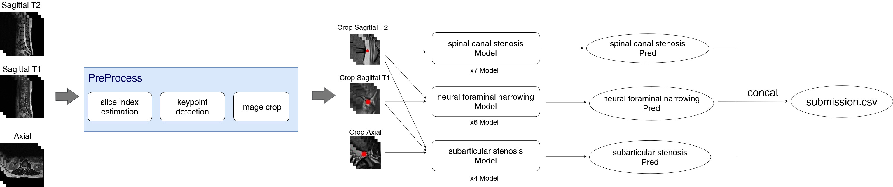
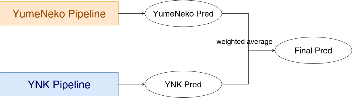
    "3013770": "# YumeNeko Pipeline Details\nHere, I will mainly explain the details of the pipeline I constructed.  \nThe score of my pipeline alone is as follows.  \n  * CV\n      * spinal canal stenosis (including any_severe_loss): 0.258\n      * neural foraminal narrowing: 0.485\n      * subarticular stenosis: 0.540\n      * overall: 0.385\n  * LB\n      * public: 0.37\n      * private: 0.42\n\n\n## Preprocess\n### Slice index estimation\nFor each viewpoint image, I estimated the slice index using a rule-based approach.   In constructing the rule-based system, I referenced several useful public notebooks. I would like to express my deep gratitude to the authors who made these resources available.\n* Sagittal T2\n  * I used the slice located at exactly half of the total number of slices (data_num//2).\n* Sagittal T1\n  * I estimated whether the index was right-to-left or left-to-right based on the positional relationship with the Axial images from the same study_id.\n  * In the case of right-to-left, I used the slice at right_instance_number = int(data_num * 0.274) and left_instance_number = int(data_num * 0.719). For left-to-right, the slices are reversed.\n  * Alignment with the Axial image was done using this public Notebook.\n    https://www.kaggle.com/code/vaillant/cross-reference-images-in-different-mri-planes?scriptVersionId=182551992\n* Axial  \n  * From the key points at each level of the Sagittal T2 predicted using the method described later, I calculated the corresponding slice range for each level and the slice ID closest to the Sagittal T2 key points.\n  * This process used this public Notebook.  \n    https://www.kaggle.com/code/hengck23/ver-1-demo-workflow-2-stage-approach?scriptVersionId=191553260\n\n### Key Point Prediction\n* I used a simple regression model, which connects N fully connected layers to a backbone from timm, to make predictions.  \n  * Input: Slice image (1ch) of index estimated by the above rule base\n  * Output: N relative coordinates of key points corresponding to each level (Sagittal T1/T2: N=5, Axial: N=2).  \n* I trained the model independently for each viewpoint image.\n  * Both backbones are EfficientNet-b3\n* I adopted l1_loss, and the average val_loss ranged between 0.008 and 0.015. However, in practice, there were several cases where the positions were shifted at the level unit. I believe there is considerable room for improvement, but due to time constraints, I was unable to dedicate time to refining this process, so I had to compromise.\n\n### image crop\n* One of the following crops was used for each viewpoint image\n1. Sagittal overall crop  \n   * A crop that includes the regions of all levels from l1/l2 to l5/s1.\n   * The crop range was determined by adding margins to the predicted y-coordinates of l1/l2 and l5/s1.  \n   ![](https://www.googleapis.com/download/storage/v1/b/kaggle-forum-message-attachments/o/inbox%2F3823496%2F7ab1648bd05500b71dbc3e43245f1df9%2Fwhole_crop.jpg?generation=1728568738331341&alt=media)\n\n2. Sagittal level crop  \n   * Crop the area corresponding to each level   \n   * The crop region was determined based on the distance between the y-coordinate of the target level and the y-coordinates of the levels above and below it.\n   ![](https://www.googleapis.com/download/storage/v1/b/kaggle-forum-message-attachments/o/inbox%2F3823496%2F1cd09e13ace6e9ef7d4ec0abeea25e62%2Flevel_crop3_resize.jpg?generation=1728568794192947&alt=media)\n    \n3. Axial crop\n   * I cropped the region near the coordinates to divide the right and left sides.\n   * I divided the image into right and left halves using the midpoint of the x-coordinates of the estimated right_point and left_point, then cropped it to form a square.\n   ![](https://www.googleapis.com/download/storage/v1/b/kaggle-forum-message-attachments/o/inbox%2F3823496%2Fb6060837ecb4534da4aec1716f0f9f93%2Faxial_crop_resize.jpg?generation=1728568716681437&alt=media)\n  \n## Label classification\n### Outline\n* I used a 2.5D model that takes as input images where 3 to 5 slices, centered around the slice index determined during preprocessing, are stacked in the channel direction.\n* Basically, I used the following viewpoint images for each condition, but some models introduced diversity by using multiple viewpoint images as input:\n  * spinal canal stenosis: Sagittal T2\n  * neural_foraminal_narrowing: Sagittal T1\n  * subarticular_stenosis: Axial T2\n* The input image size was resized to 512x512.\n* During training, I applied augmentation by randomly increasing or decreasing the slice index within a range of ±2.\n* During training, ground truth key points were used, and predicted key points were used for cv score calculations.\n* For submission, I used the weights trained on all data.\n\n### spinal canal stenosis model\n\n| # | Input | Output | backbone | CV |\n| --- | --- | --- | --- | --- |\n| 1  | SagT2 overall_crop 5ch | all level class（5level * 3class） | EfficientNet-b3 | 0.326 |\n| 2 | SagT2 level_crop 3ch | class per level（3class） | EfficientNet-b4 | 0.288 |\n| 3 | SagT2 level_crop 5ch | class per level（3class） | EfficientNet-b4 | 0.284 |\n| 4 | SagT2 level_crop 5ch | class per level（3class） | MaxViT tiny | 0.273 |\n\n* Spinal canal stenosis was predicted using only Sagittal T2 images. Although I also tried building a model that took Axial images as input, it did not show any improvement when ensemble methods were applied, so I did not adopt it.\n* In model #1, I split the input by each channel and fed them into the backbone to extract features for each slice, then applied LSTM in the head to capture features between the slices.\n\n### neural_foraminal_narrowing model\n\n| # | Input | Output | backbone | CV |\n| --- | --- | --- | --- | --- |\n| 1  | SagT1 overall_crop 5ch | all level class（5level * 3class） | EfficientNet-b3 | 0.531 |\n| 2 | SagT1 level_crop 3ch+SagT2 level crop 3ch | class per level（3class） | MaxViT tiny | 0.506 |\n| 3 | SagT1 level_crop 3ch + SagT2 level_crop 3ch | all level class（5level * 3class） | EfficientNet-b3 | 0.512 |\n\n* Right and left sides were not distinguished and were trained together.\n* For models #2 and #3, I applied the same slice index and crop range used for Sagittal T1 to the Sagittal T2 images of the same study_id, stacking them in the channel direction and using both viewpoint images as input.\n* In model #3, I passed cropped images of each level from the same slice through the backbone to obtain feature vectors. After applying self-attention to the obtained feature vectors, they were fed into the level-specific heads to predict the class for all levels simultaneously.\n  * By reusing the backbone weights from the model trained in #2, the final accuracy improved slightly.\n![](https://www.googleapis.com/download/storage/v1/b/kaggle-forum-message-attachments/o/inbox%2F3823496%2Fbe36b8857973ef4af892dfd11b6ae7c0%2FT1_model3.jpg?generation=1728568882650300&alt=media)\n\n\n### subarticular_stenosis model\n\n| # | Input | Output | backbone | CV |\n| --- | --- | --- | --- | --- |\n| 1 | Axial crop 3ch | class per level（3class） | MaxViT tiny | 0.549 |\n| 2 | Axial crop 3ch & SagT1 level_crop 3ch + SagT2 level_crop 3ch | class per level（3class） | EfficientNet-b3 | 0.551 |\n\n* For subarticular stenosis, I only used the level-cropped images. I also experimented with a model that generated an overall cropped image from the Axial view and output Right/Left simultaneously, but the accuracy of the single model was not good, and it did not improve when included in the ensemble, so I did not adopt it.\n* In model #2, I input Axial and Sagittal images into separate backbones to extract features, then concatenated them before passing through the head to predict the labels.\n![](https://www.googleapis.com/download/storage/v1/b/kaggle-forum-message-attachments/o/inbox%2F3823496%2Feae1a654f562e1f46f61a8d583e6326b%2FSS_model1.jpg?generation=1728568908720665&alt=media)\n\n\n## Not Working\n* Puseudo Label\n  * I tried augmenting the training data by applying pseudo-labels to external data, but it did not significantly improve accuracy.\n  * I experimented with various patterns, such as using the model's inference results as soft labels and using annotations that my teammate manually labeled as hard labels, but I was unable to effectively utilize them.\n\n* Noisy Label Removal\n  * My teammates noticed that some annotation labels were noisy, so I calculated the log_loss for each sample and excluded samples with significantly high losses from the training data. However, the local score uniformly worsened, so we did not adopt this approach.\n  * That said, there seemed to be top-ranking teams, including the second-place team, that improved their scores by removing noisy data. So, if we had refined the removal method further, it might have had a significant positive impact.\n\n* And much more...",
    "3014910": "# YNK Pipeline Naoya Part\n\nI would like to express deepest gratitude to Kagglen and RSNA for providing an incredible platform to grow as a data scientist. I am also immensely thankful to my amazing team members, whose collaboration and insights were invaluable throughout this journey.\n\n## Score\n\nThe score of my pipeline is as follows.\n* CV\n    * neural foraminal narrowing (two ensemble models): 0.486\n    * subarticular stenosis (single model): 0.573\n\n## Preprocess\n\nThe preprocessing for the YNK pipeline was mainly handled by @kurimats, so please refer to his work. As for myself, I was responsible for the 2.5D segmentation of interbertebral discs by level.<br>\nWe used the output from [TotalSegmentator MRI](https://github.com/wasserth/TotalSegmentator) as the mask image. To avoid under extraction, we finally selected the central 7 slices as the input. The model used was U-Net, and the backbone was tf_efficientnet_b5.ns_jft_in1k. <br>\n\nAn example of intervertebral disc segmentation result.<br>\n![](https://www.googleapis.com/download/storage/v1/b/kaggle-forum-message-attachments/o/inbox%2F13621367%2F68c13731b179b7b3e997adb4fb75f1bf%2Fgray_image_rgb.png?generation=1728668173919534&alt=media)\n\n## Neural Foraminal Narrowing\n\n* During both training and inference, we predicted the annotated slice and used a total of three slices, including one slice before and one slice after. \n* I trained without distinguishing between left and right. \n* I used only Sagittal T1 images (3 slices).\n* experimental conditions\n    * model: 2D-based model + LSTM\n    * split: 5-fold split to ensure an equal number of severe cases in each fold.\n    * augmentation: cutmix, mixup, vertical flip, geometric distortions, coarse dropout\n    * input size: 256x256\n\n|#|backbone|CV|\n|---|:---:|:---:|\n|1|tf_efficientnetv2_s.in21k_ft_in1k|0.494|\n|2|swin_small_patch4_window7_224.ms_in22k_ft_in1k|0.494|\n\nAn example of cropped image.\n<img src=\"https://www.googleapis.com/download/storage/v1/b/kaggle-forum-message-attachments/o/inbox%2F13621367%2F58c21839c28d95809863d47869f6f9dd%2Fnfn.png?generation=1728668422021879&alt=media\", width='256'>\n\n\n## Subarticular Stenosis\n\n* During both training and inference, axial slices were selected based on DICOM header information, choosing the slice closest to the predicted Spinal Canal Stenosis point. \n* For study_id with multiple axial series, a separate dataset was created for each series, and inference was performed on each. The outputs were then ensembled by taking a simple average.\n* I used only Axial T2 images (5 slices).\n* I trained without distinguishing between left and right. \n* experimental conditions\n    * model: 2D-based model + LSTM\n    * split: 5-fold split to ensure an equal number of severe cases in each fold.\n    * augmentation: cutmix, mixup, horizontal flip, geometric distortions, coarse dropout\n    * input size: 256x256\n\n|#|backbone|CV|\n|---|:---:|:---:|\n|1|tf_efficientnetv2_s.in21k_ft_in1k|0.573|\n\n\nAn example of cropped image.\n<img src=\"https://www.googleapis.com/download/storage/v1/b/kaggle-forum-message-attachments/o/inbox%2F13621367%2F42dde2f2bc08eac3af96616cd748e526%2Fss.png?generation=1728668610623567&alt=media\", width='256'>",
    "3014719": "\n# YNK Pipeline kurimats Part\n\nFirst of all, we would like to express our sincere gratitude to the organizers and the Kaggle team for arranging such an intriguing and challenging competition. We are honored to have achieved results in this competition.\n\nIn our approach, I was responsible for preprocessing, while @takashimanaoya and @yosukeyama handled the modeling. Additionally, the pipeline was created based on advice from both of them.\n\nWe adopted a 2-stage approach for preprocessing: disc segmentation to predict the cropping area and slice classification to predict annotation slices at each level. Since our pipeline does not rely on GT coordinates, we believe it contributed to significant accuracy improvements when ensembled with the @kashiwaba pipeline.\n\n## Spinal Canal Stenosis (SCS)\n\n**Stage 1**:  \nI retrained the TotalSegmentator model and performed 5-class segmentation. I am grateful to the author of the total-mr model for providing such an accurate segmentation model.  Link: [TotalSegmentator](https://github.com/wasserth/TotalSegmentator)\n\nSince disc segmentation from sagittal T2 images was unstable, I used sagittal T1 images for segmentation. Using the header information, I determined the crop positions for sagittal T2 images. Below are the cropping methods for each level and the CSC prediction points calculated by the rule-based approach.\n![](https://www.googleapis.com/download/storage/v1/b/kaggle-forum-message-attachments/o/inbox%2F18982014%2Fa5ece59c5222971082747ae6977465f6%2F2024-10-10%20101158.png?generation=1728656408944721&alt=media)\n**Stage 2**:  \nSlice classification was used to predict the annotation slices for each level. Even in cases where the spine was curved, we were able to consistently capture the center of each level. We used three sagittal T2 images centered on this point, and @yosukeyama performed the predictions.\n\n## Subarticular Stenosis (SS)\n\nBased on the SCS predicted coordinates mentioned above, the nearest axial image was selected. If the second closest image had a different orientation, we obtained axial slices from two orientations. For each orientation, five slices centered on the middle slice were used to build the dataset. Crops were taken from both sides of the SCS prediction points in the selected axial slices, and @takashimanaoya performed the predictions.\n\nAdditionally, we had a model that used only sagittal images. We created a dataset of about five sagittal slices, starting from the center of the spine and moving outward, and @yosukeyama performed the predictions.\n\n## Neural Foraminal Narrowing (NFN)\n\nFor NFN, the same process as for SCS was applied. We identified the central NFN crop on both the left and right sides for each level, and using five slices centered on the identified slice, @takashimanaoya and @yosukeyama performed the predictions.\n\nA detailed explanation of the models used will be provided later by the two of them.",
    "3016707": "# YYama part\n\nFirstly, I would like to express my gratitude to the competition organizers. I've participated in many competitions, but this was the first one I fully completed in a year and a half. Kaggle is truly exciting!\n\n\nI built my model based on the preprocessed data provided by @kurimats. For my model, NFN and SS were predicted together using a single model, while SCS was predicted with a separate model.\n\n## NFN, SS\nI stacked seven images and predicted NFN and SS simultaneously. Since NFN and SS are anatomically close to each other, predicting them together allows the model to learn to distinguish between them more effectively. I only used sagittal T1 and T2 images for training. T1 and T2 were treated as separate stacks, and predictions were made for each. The final prediction for NFN was based on the T1 output only, while SS used the average of T1 and T2 predictions. These decisions were made based on cross-validation (CV) scores.\n\nThe model architecture is as follows:\n```\nclass NFN_SS_MIL_Model(nn.Module):\n    def __init__(self, base_model='tf_efficientnet_b0_ns', pool=\"avg\", pretrain=True):\n        super(NFN_SS_MIL_Model, self).__init__()\n        self.model = timm.create_model(base_model, pretrained=pretrain, num_classes=0, in_chans=3)\n        nc = self.model.num_features\n        self.gru = nn.GRU(nc, 512, bidirectional=True, batch_first=True, num_layers=2)\n        self.exam_predictor = nn.Linear(512*2, CFG.target_size)\n        self.pool = nn.AdaptiveAvgPool1d(1)\n\n    def forward(self, input1):\n        shape = input1.size()\n        batch_size = shape[0]\n        n = shape[1]\n        input1 = input1.view(-1,shape[2],shape[3],shape[4])\n        x =  self.model(input1)    \n        embeds, _ = self.gru(x.view(batch_size,n,x.shape[1]))\n        embeds = self.pool(embeds.permute(0,2,1))[:,:,0]\n        y = self.exam_predictor(embeds)\n        return y\n```\n\n## SCS\nThis model was designed solely to predict SCS. Preliminary experiments showed that adding level prediction as an auxiliary target improved the CV score, so I adopted this approach. The input consisted of three stacked images, and only sagittal T2 images were used.\n\nThe model architectures are:\n- MIL model (2D backbone + 2-layer GRU)\n- 2D model (MaxViT)\n\n```\nclass SCS_MIL_MultiHead_Model(nn.Module):\n    def __init__(self, base_model='tf_efficientnet_b0_ns', num_classes1=3, num_classes2=5, pool=\"avg\", pretrain=False):\n        super(SCS_MIL_MultiHead_Model, self).__init__()\n        self.model = timm.create_model(base_model, pretrained=pretrain, num_classes=0, in_chans=1)\n        nc = self.model.num_features\n        self.gru = nn.GRU(nc, 512, bidirectional=True, batch_first=True, num_layers=2)\n        self.pool = nn.AdaptiveAvgPool1d(1)\n        \n        self.exam_predictor1 = nn.Linear(512*2, num_classes1)  \n        self.exam_predictor2 = nn.Linear(512*2, num_classes2)\n\n    def forward(self, input1):\n        shape = input1.size()\n        batch_size, n = shape[0], shape[1]\n        input1 = input1.view(-1, shape[2], shape[3], shape[4])\n        x = self.model(input1)\n        \n        embeds, _ = self.gru(x.view(batch_size, n, x.shape[1]))\n        embeds = self.pool(embeds.permute(0, 2, 1))[:, :, 0]\n        \n        y1 = self.exam_predictor1(embeds)\n        y2 = self.exam_predictor2(embeds) # aux head for level prediction\n        \n        return y1, y2\n```\n\n``` \nclass SCS_2D_MultiHead_Model(nn.Module):\n    def __init__(self, model_name, num_classes1=3, num_classes2=5, pretrained=False):\n        super(SCS_2D_MultiHead_Model, self).__init__()\n        self.base_model = timm.create_model(model_name, pretrained=pretrained, num_classes=0) \n        self.exam_predictor1 = nn.Linear(self.base_model.num_features, num_classes1)\n        self.exam_predictor2 = nn.Linear(self.base_model.num_features, num_classes2)\n\n    def forward(self, x):\n        features = self.base_model(x)\n        y1 = self.exam_predictor1(features)\n        y2 = self.exam_predictor2(features)\n        return y1, y2\n```\n\nAlthough I used only three stacked images, the MIL model improved my local CV score. The 2D model was included in the final ensemble as it contributed to improving the overall score. Different 2D backbones were used in the ensemble to enhance performance by leveraging the diversity of the backbones.\n\n| 2D Backbone     | MIL   | Memo             | CV Score |\n|-----------------|-------|------------------|----------|\n| MaxViT Tiny     | No    |                  | 0.278    |\n| EfficientNetV2S | Yes   |                  | 0.272    |\n| NextViT Small   | Yes   | 80% center crop  | 0.273    |\n\n## What Didn't Work Well\n\n- A lot of things didn’t go as planned.\n- The external dataset from Mendeley. I labeled 500 cases focusing on SCS, but using this data for training lowered the CV score, so I couldn’t use it for the actual submission. The RSNA dataset was likely labeled by multiple annotators, whereas my single-person labeling introduced significant bias. Additionally, the Mendeley dataset may have only contained easy cases (when we ran the Mendeley predictions using @kashiwaba 's models, the prediction resulted in a score about 0.17 on my labels).\n- Dealing with noisy labels. The RSNA dataset labels were highly noisy, with some cases labeled as \"severe\" that were clearly \"normal.\" I tried removing the cases with a significant gap between the model's predictions and the labels, and also relabeled some data based on model predictions, but the CV score worsened, so I couldn't submit these results either. The 2nd place team seemed to have success with a similar method, so there is a chance that fine-tuning the amount of data to remove or adjusting the relabeling method could have improved the score.\n",
    "3016794": "Have you tried using the Noise induction method in any of your solutions?? ",
    "3014709": "",
    "3014707": ""
  }
}