{"metadata":{"kernelspec":{"language":"python","display_name":"Python 3","name":"python3"},"language_info":{"name":"python","version":"3.10.13","mimetype":"text/x-python","codemirror_mode":{"name":"ipython","version":3},"pygments_lexer":"ipython3","nbconvert_exporter":"python","file_extension":".py"},"kaggle":{"accelerator":"none","dataSources":[{"sourceId":71549,"databundleVersionId":8561470,"sourceType":"competition"}],"dockerImageVersionId":30715,"isInternetEnabled":true,"language":"python","sourceType":"notebook","isGpuEnabled":false}},"nbformat_minor":4,"nbformat":4,"cells":[{"cell_type":"markdown","source":"The goal of this competition is to create models that can be used to aid in the **detection** and **classification** of degenerative spine conditions using lumbar spine **MR images**","metadata":{}},{"cell_type":"markdown","source":"# Theory","metadata":{}},{"cell_type":"markdown","source":"## Lumbar region","metadata":{}},{"cell_type":"markdown","source":"<center><img src=\"https://rojehmelikianmd.com/wp-content/uploads/2020/05/rojmd-lumbar-spine.jpg\"/><img src=\"https://my.clevelandclinic.org/-/scassets/images/org/health/articles/17499-spinal-stenosis-01?io=transform:fit,width:780\"></center>","metadata":{}},{"cell_type":"markdown","source":"Comprises $5$ vertebral bodies, at the **lower back**.\n\nWith side view: Between the **vertebral bodies** has **intervertebral discs** (These discs are cartilage structures that serve as cushions, absorbing shock and facilitating movement).\n\nWith top view: For each vertebral body is the **spinal canal** (The spinal cord is a bundle of nerves that transmits signals between the brain and the rest of the body).","metadata":{}},{"cell_type":"markdown","source":"## Magnetic Resonance Imaging (MRI)","metadata":{}},{"cell_type":"markdown","source":"<center><img src=\"https://i.postimg.cc/MxG2zJMZ/CT-Image-Planes.jpg\"></center>","metadata":{}},{"cell_type":"markdown","source":"## ","metadata":{}},{"cell_type":"markdown","source":"A typical MRI of the lumbar spine might look as <a href=\"https://radiopaedia.org/articles/lumbar-spine-protocol-mri\">follows</a>:\n\n**sagittal images**:\n* angulation: parallel to the lumbar spinal axis and spinous processes\n* volume: includes the whole vertebral bodies and the facet joints\n* slice thickness: ≤3 mm\n\n**coronal images**:             \n* angulation: parallel to the lumbar spinal axis and transverse processes\n* volume: includes the whole vertebral body spinal canal and posterior laminae\n* slice thickness: ≤3 mm\n\n**axial images (long stack)**:\n* angulation: perpendicular to the lumbar spine\n* volume:\n\n$\\hspace{1cm}$- variable depends on the clinical question and/or the visible pathology \\\n$\\hspace{1cm}$- if clinical indication is generic, sufficient to include upper block (inferior half of L3 to superior half of L5) and lower block (inferior half of L5 to superior half of sacrum) \\\n$\\hspace{1cm}$- ensure slices intersect perpendicularly with nucleus pulposus\n* slice thickness: ≤3 mm\n\n**axial images (short stacks)**:\n* angulation: parallel to the intervertebral discs in question\n* volume: variable depends on the clinical question and/or the visible pathology\n* slice thickness: ≤3 mm","metadata":{}},{"cell_type":"markdown","source":"## Standard sequences","metadata":{}},{"cell_type":"markdown","source":"<center><img src=\"https://www.radiology.expert/content/images/modules/MRI%20lumbar%20spine/Eng/resized/RadiologyExpert_Ned_Module_MRI_LWK_fig05_Module_MRI%20LWK_verschillende%20MRI%20sequenties%20herkennen2_OVERLAY_640x0.jpg\"></center>","metadata":{}},{"cell_type":"markdown","source":"**T1-weighted**\n* purpose: bone and/or soft-tissue characterization\n* technique:  T1 fast spin echo\n* planes: sagittal, axial* (optional)\n\n**T2-weighted**\n* purpose: bone and/or soft-tissue characterization, detailed anatomy, including ligament and tendon anatomy\n* technique: T2 Dixon / T2 fast spin echo\n* planes: coronal, sagittal, axial\n\n**T2-weighted (fat-saturated)**\n* purpose: bone and soft tissue characterization, assessment of inflammatory changes, fractures\n* technique: T2 Dixon / STIR / T2 FS fast spin echo,\n* planes: coronal or sagittal, axial*","metadata":{}},{"cell_type":"markdown","source":"## Foraminal Narrowing","metadata":{}},{"cell_type":"markdown","source":"Label            |  Describe\n:-------------------------:|:-------------------------:\n![](https://i.imgur.com/6c7erNM.png)  |  ![](https://i.imgur.com/b1VGiN5.png)","metadata":{}},{"cell_type":"markdown","source":"Foraminal narrowing results in nerve compression, leading to pain along the affected nerve's distribution, which is the path the nerve travels in the body.","metadata":{}},{"cell_type":"markdown","source":"## Subarticular Stenosis","metadata":{}},{"cell_type":"markdown","source":"Label            |  Describe\n:-------------------------:|:-------------------------:\n![](https://files.miamineurosciencecenter.com/media/filer_public_thumbnails/filer_public/d5/08/d508ae6a-a4f2-4796-be9f-455f8df45fe1/herniation_zones.jpg__1700.0x1308.0_q85_subject_location-850%2C656_subsampling-2.jpg)  |  ![](https://i.imgur.com/Usuxgge.png)","metadata":{}},{"cell_type":"markdown","source":"The compression in this zone is often due to similar factors that cause foraminal narrowing.","metadata":{}},{"cell_type":"markdown","source":"## Canal Stenosis","metadata":{}},{"cell_type":"markdown","source":"Label            |  Describe\n:-------------------------:|:-------------------------:\n![](https://prod-images-static.radiopaedia.org/images/940993/f7a8adca63efae788f621869cc21e8_big_gallery.jpg)  |  ![](https://i.imgur.com/opjnAwl.png)","metadata":{}},{"cell_type":"markdown","source":"Canal stenosis involves impingement of the spinal canal, the passageway through which the spinal cord travels.","metadata":{}},{"cell_type":"markdown","source":"summary","metadata":{}},{"cell_type":"markdown","source":"<img src=\"https://pbs.twimg.com/media/GG3d1CMakAAXzMj?format=jpg&name=4096x4096\"/>","metadata":{}},{"cell_type":"markdown","source":"<img src=\"https://ar5iv.labs.arxiv.org/html/1807.10215/assets/severity_examples_new2.png\"/>","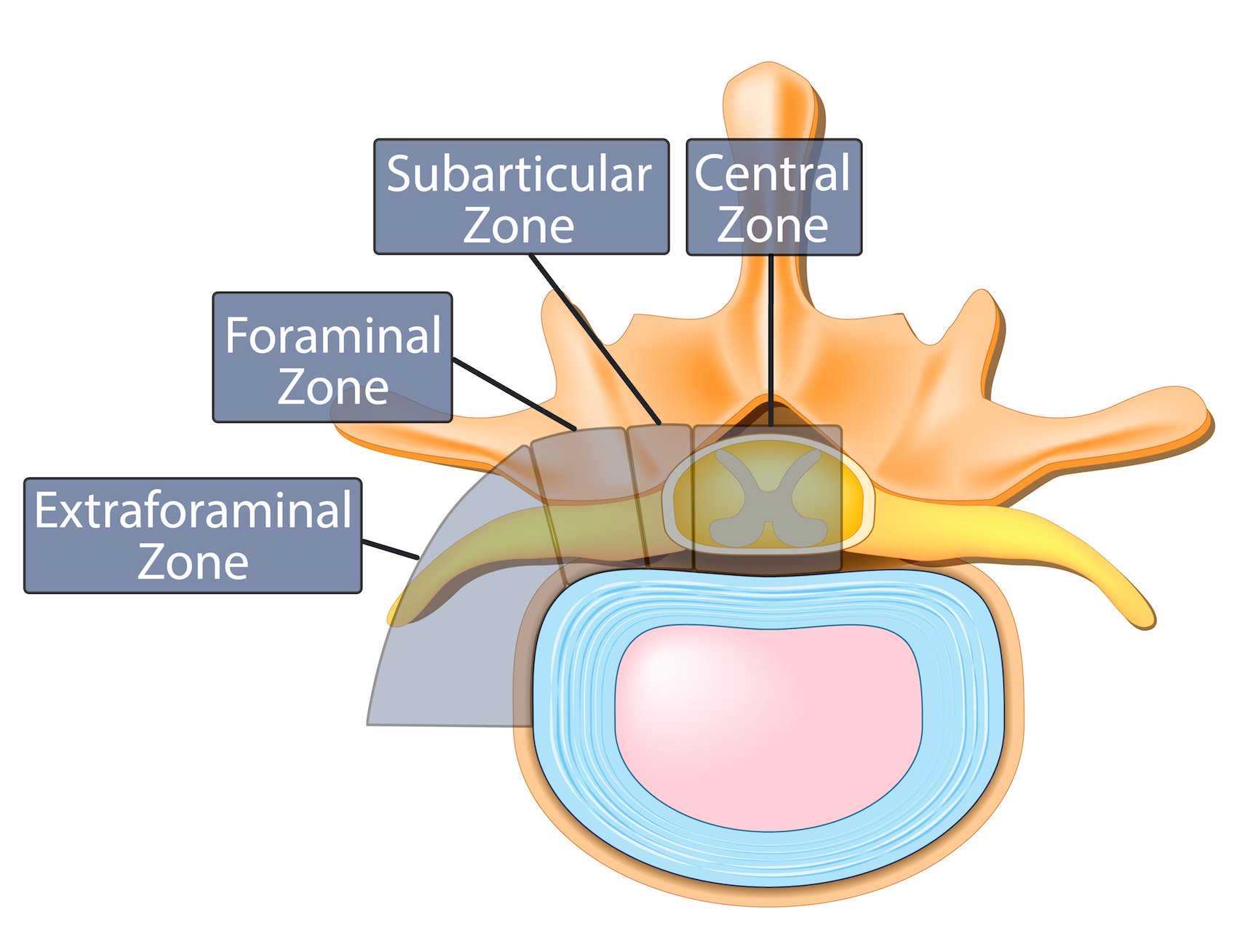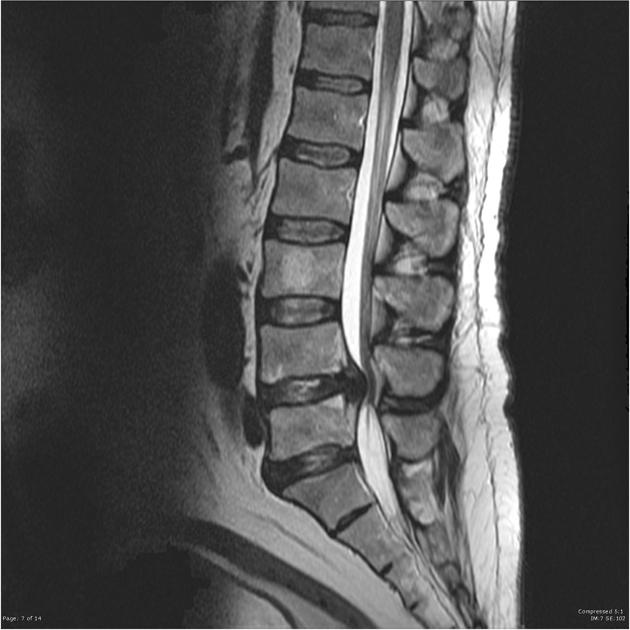metadata":{}},{"cell_type":"markdown","source":"# Dataset overview","metadata":{}},{"cell_type":"markdown","source":"The dataset is made up of roughly $2000$ MR studies. Spine radiology specialists have provided annotations to indicate the presence, vertebral level and location of any cervical spine stenosis.\n\nThe focus of the challenge is on classifiying five specific lumbar spine degenerative conditions:\n- Left Neural Foraminal Narrowing\n- Right Neural Foraminal Narrowing\n- Left Subarticular Stenosis\n- Right Subarticular Stenosis\n- Spinal Canal Stenosis\n\nFor each imaging study in the dataset, severity scores (**Normal/Mild**, **Moderate**, or **Severe**) are provided for each of these five conditions across the intervertebral disc levels:\n- L1/L2\n- L2/L3\n- L3/L4\n- L4/L5\n- L5/S1","metadata":{}},{"cell_type":"markdown","source":"The two main image are the **axial** and **sagittal planes**.\n\n- **Axial plane**: Horizontal slices perpendicular to the spine.\n- **Sagittal plane**: Vertical slices parallel to the spine.\n\nThe two variants are **T1** weighted or **T2** weighted. \n\n- **T1**: weighted images show fat as being brighter. The inner part of bones would appear brighter on **T1** images.\n- **T2**: images show water as brighter. The spinal canal would appear as brighter on **T2** images.","metadata":{}},{"cell_type":"markdown","source":"# EDA","metadata":{}},{"cell_type":"code","source":"%cd /kaggle/input/rsna-2024-lumbar-spine-degenerative-classification\n!ls -l","metadata":{"execution":{"iopub.status.busy":"2024-06-25T06:55:41.795940Z","iopub.execute_input":"2024-06-25T06:55:41.796515Z","iopub.status.idle":"2024-06-25T06:55:42.953789Z","shell.execute_reply.started":"2024-06-25T06:55:41.796462Z","shell.execute_reply":"2024-06-25T06:55:42.952091Z"},"trusted":true},"execution_count":null,"outputs":[]},{"cell_type":"markdown","source":"## Directory Structure","metadata":{}},{"cell_type":"markdown","source":"```lua\n├── /kaggle/working\n└── /kaggle/input/rsna-2024-lumbar-spine-degenerative-classification/\n    ├── test_images/\n    │   ├── 1005139/\n    │   │   └── 609308237/\n    │   │       ├── 1.dcm\n    │   │       └── ...\n    │   └── ...\n    ├── test_series_descriptions.csv\n    ├── train_images/\n    │   ├── 4003253/\n    │   │   └── 702807833/\n    │   │       ├── 1.dcm\n    │   │       └── ...\n    │   └── ...\n    ├── train_label_coordinates.csv\n    ├── train_series_descriptions.csv\n    └── train.csv\n```","metadata":{}},{"cell_type":"markdown","source":"## Dataset composition","metadata":{}},{"cell_type":"markdown","source":"The training dataset consists of $1975$ rows (each row is a study)\n\nEach study may include multiple series of images\n\nEach study maps to target labels, such as **spinal_canal_stenosis_l1_l2**, with the severity levels of **Normal/Mild**, **Moderate**, or **Severe**. Some entries have incomplete labels.\n\nThe test dataset contains approximately $500$ rows/studies (speculative based on host saying the dataset was $~2500$ studies)","metadata":{}},{"cell_type":"markdown","source":"## File descriptions","metadata":{}},{"cell_type":"markdown","source":"<b><code>train.csv</code></b>:\n* Contains labels for the training set. Each record includes:\n    - <b><code>study_id</code> (string):</b> The study ID. \n        - Each study may include multiple series of images.\n    - <b><code>[condition]_[level]</code> (string):</b> The target labels, such as... \n        - **`spinal_canal_stenosis_l1_l2`**, with severity levels of **`Normal/Mild`**, **`Moderate`**, or **`Severe`**. \n        - Some entries have incomplete labels.\n\n<b><code>train_label_coordinates.csv</code></b>:\n* Provides the coordinates for labeled regions. Each record includes:\n    - <b><code>study_id</code> (string):</b> The study ID.\n    - <b><code>series_id</code> (string):</b> The imagery series ID.\n    - <b><code>instance_number</code> (int):</b> The image's order number within the 3D stack.\n    - <b><code>condition</code> (string):</b> The core condition, which can be one of...\n        - **`spinal_canal_stenosis`**\n        - **`neural_foraminal_narrowing`** [considered for each side of the spine]\n        - **`subarticular_stenosis`** [considered for each side of the spine]\n    - <b><code>level</code> (string):</b> The relevant vertebrae, such as **`l3_l4`**.\n    - <b><code>x</code> (float):</b> The x-coordinate for the center of the labeled area.\n    - <b><code>y</code> (float):</b> The y-coordinate for the center of the labeled area.\n\n<b><code>sample_submission.csv</code></b>:\n* Provides a format template for submissions. Each record includes:\n    - <b><code>row_id</code> (string):</b> A slug of the study ID, condition, and level, such as `12345_spinal_canal_stenosis_l3_l4`.\n    - <b><code>normal_mild</code> (float):</b> The predicted probability for the Normal/Mild severity level.\n    - <b><code>moderate</code> (float):</b> The predicted probability for the Moderate severity level.\n    - <b><code>severe</code> (float):</b> The predicted probability for the Severe severity level.\n\n<b><code>[train/test]_images/[study_id]/[series_id]/[instance_number].dcm</code></b>:\n* The directory structure for the imagery data.\n\n<b><code>[train/test]_series_descriptions.csv</code></b>:\n* Contains descriptions of the scan series. Each record includes:\n    - <b><code>study_id</code> (string):</b> The study ID.\n    - <b><code>series_id</code> (string):</b> The series ID.\n    - <b><code>series_description</code> (string):</b> The scan's orientation.\n\n<br>","metadata":{}},{"cell_type":"markdown","source":"## Loading Diagnosis Information","metadata":{}},{"cell_type":"code","source":"import os\nimport missingno as msno\nimport pandas as pd\nimport matplotlib.pyplot as plt\nimport cv2\nimport warnings\nimport pydicom\nimport numpy as np\nimport random\n\nfrom mpl_toolkits.axes_grid1.inset_locator import zoomed_inset_axes\nfrom mpl_toolkits.axes_grid1.inset_locator import mark_inset\nfrom math import ceil\nfrom glob import glob\nfrom matplotlib import animation, rc\nimport matplotlib.patches as patches\nfrom pydicom.pixel_data_handlers.util import apply_voi_lut\nfrom tqdm.notebook import tqdm\n\ntqdm.pandas()\n%matplotlib inline","metadata":{"execution":{"iopub.status.busy":"2024-06-26T03:57:36.058591Z","iopub.execute_input":"2024-06-26T03:57:36.059003Z","iopub.status.idle":"2024-06-26T03:57:37.916494Z","shell.execute_reply.started":"2024-06-26T03:57:36.058972Z","shell.execute_reply":"2024-06-26T03:57:37.915279Z"},"trusted":true},"execution_count":null,"outputs":[]},{"cell_type":"code","source":"class TextColor():\n    def __init__(self):\n        self.B = '\\033[94m'\n        self.Y = '\\033[93m'\n        self.G = '\\033[92m'\n        self.R = '\\033[91m'\n        self.BD = '\\033[1m'\n        self.E = '\\033[0m'\n\n    def RED(self, msg='ERROR'):\n        return self.R + str(msg) + self.E\n\n    def GREEN(self, msg='SUCCESS'):\n        return self.G + str(msg) + self.E\n\n    def YELLOW(self, msg='WARNING'):\n        return self.Y + str(msg) + self.E\n\n    def BLUE(self, msg=''):\n        return self.B + f\"{msg}\" + self.E\n\n    def BOLD(self, msg=''):\n        return self.BD + f\"{msg}\" + self.E\n    \n    def print_var(self, **kwargs):\n        for var, value in kwargs.items():\n            print(f'➤ {self.GREEN(var)} = {self.BOLD(value)}')\n        print()\nclr = TextColor()","metadata":{"execution":{"iopub.status.busy":"2024-06-26T03:57:37.918694Z","iopub.execute_input":"2024-06-26T03:57:37.919606Z","iopub.status.idle":"2024-06-26T03:57:37.931590Z","shell.execute_reply.started":"2024-06-26T03:57:37.919553Z","shell.execute_reply":"2024-06-26T03:57:37.930481Z"},"trusted":true},"execution_count":null,"outputs":[]},{"cell_type":"code","source":"files = glob('/kaggle/input/rsna-2024-lumbar-spine-degenerative-classification/*.csv')\npaths = {path.split('/')[-1].split('.')[0]:path for path in files}\npaths","metadata":{"_uuid":"8f2839f25d086af736a60e9eeb907d3b93b6e0e5","_cell_guid":"b1076dfc-b9ad-4769-8c92-a6c4dae69d19","execution":{"iopub.status.busy":"2024-06-26T03:57:37.933144Z","iopub.execute_input":"2024-06-26T03:57:37.933486Z","iopub.status.idle":"2024-06-26T03:57:37.949419Z","shell.execute_reply.started":"2024-06-26T03:57:37.933456Z","shell.execute_reply":"2024-06-26T03:57:37.948048Z"},"trusted":true},"execution_count":null,"outputs":[]},{"cell_type":"markdown","source":"### train.csv","metadata":{}},{"cell_type":"code","source":"df_train = pd.read_csv(paths['train'])\nclr.print_var(**{'Shape of data': df_train.shape})\ndf_train.head(5)","metadata":{"execution":{"iopub.status.busy":"2024-06-26T03:57:39.950050Z","iopub.execute_input":"2024-06-26T03:57:39.950469Z","iopub.status.idle":"2024-06-26T03:57:40.024352Z","shell.execute_reply.started":"2024-06-26T03:57:39.950439Z","shell.execute_reply":"2024-06-26T03:57:40.023016Z"},"trusted":true},"execution_count":null,"outputs":[]},{"cell_type":"code","source":"df_train.info()","metadata":{"execution":{"iopub.status.busy":"2024-06-25T06:55:43.106920Z","iopub.execute_input":"2024-06-25T06:55:43.107275Z","iopub.status.idle":"2024-06-25T06:55:43.149341Z","shell.execute_reply.started":"2024-06-25T06:55:43.107237Z","shell.execute_reply":"2024-06-25T06:55:43.147741Z"},"trusted":true},"execution_count":null,"outputs":[]},{"cell_type":"code","source":"df_train.describe(include='object').T","metadata":{"execution":{"iopub.status.busy":"2024-06-25T06:55:43.151249Z","iopub.execute_input":"2024-06-25T06:55:43.151735Z","iopub.status.idle":"2024-06-25T06:55:43.220186Z","shell.execute_reply.started":"2024-06-25T06:55:43.151696Z","shell.execute_reply":"2024-06-25T06:55:43.218577Z"},"trusted":true},"execution_count":null,"outputs":[]},{"cell_type":"code","source":"msno.bar(df_train)\nplt.show()","metadata":{"execution":{"iopub.status.busy":"2024-06-25T06:55:43.222105Z","iopub.execute_input":"2024-06-25T06:55:43.222682Z","iopub.status.idle":"2024-06-25T06:55:45.772027Z","shell.execute_reply.started":"2024-06-25T06:55:43.222649Z","shell.execute_reply":"2024-06-25T06:55:45.770446Z"},"trusted":true},"execution_count":null,"outputs":[]},{"cell_type":"markdown","source":"> Missing data is at **subarticular_stenosis**","metadata":{}},{"cell_type":"code","source":"figure, axis = plt.subplots(1,3, figsize=(20,5)) \nfor idx, d in enumerate(['foraminal', 'subarticular', 'canal']):\n    diagnosis = list(filter(lambda x: x.find(d) > -1, df_train.columns))\n    dff = df_train[diagnosis]\n    with warnings.catch_warnings():\n        warnings.simplefilter(action='ignore', category=FutureWarning)\n        value_counts = dff.apply(pd.value_counts).fillna(0).T\n    value_counts.plot(kind='bar', stacked=True, ax=axis[idx])\n    axis[idx].tick_params(axis='x', labelrotation=80)\n    axis[idx].set_title(f'{d} distribution')\nplt.show()","metadata":{"execution":{"iopub.status.busy":"2024-06-25T07:21:50.222336Z","iopub.execute_input":"2024-06-25T07:21:50.222797Z","iopub.status.idle":"2024-06-25T07:21:51.526618Z","shell.execute_reply.started":"2024-06-25T07:21:50.222763Z","shell.execute_reply":"2024-06-25T07:21:51.524723Z"},"trusted":true},"execution_count":null,"outputs":[]},{"cell_type":"markdown","source":"Many of our patients have **normal/mild** grades for each of the diagnoses categories.","metadata":{}},{"cell_type":"code","source":"","metadata":{"trusted":true},"execution_count":null,"outputs":[]},{"cell_type":"markdown","source":"### train_label_coordinates.csv","metadata":{}},{"cell_type":"code","source":"df_train_label = pd.read_csv(paths['train_label_coordinates'])\nclr.print_var(**{'Shape of data': df_train_label.shape})\ndf_train_label.head(5)","metadata":{"execution":{"iopub.status.busy":"2024-06-26T03:57:45.209686Z","iopub.execute_input":"2024-06-26T03:57:45.210136Z","iopub.status.idle":"2024-06-26T03:57:45.354513Z","shell.execute_reply.started":"2024-06-26T03:57:45.210101Z","shell.execute_reply":"2024-06-26T03:57:45.353284Z"},"trusted":true},"execution_count":null,"outputs":[]},{"cell_type":"code","source":"df_train_label.info()","metadata":{"execution":{"iopub.status.busy":"2024-06-25T06:55:47.239464Z","iopub.execute_input":"2024-06-25T06:55:47.239939Z","iopub.status.idle":"2024-06-25T06:55:47.267692Z","shell.execute_reply.started":"2024-06-25T06:55:47.239904Z","shell.execute_reply":"2024-06-25T06:55:47.266325Z"},"trusted":true},"execution_count":null,"outputs":[]},{"cell_type":"code","source":"df_train_label.iloc[:,2:].describe(include='all')","metadata":{"execution":{"iopub.status.busy":"2024-06-25T06:55:47.269324Z","iopub.execute_input":"2024-06-25T06:55:47.269889Z","iopub.status.idle":"2024-06-25T06:55:47.345067Z","shell.execute_reply.started":"2024-06-25T06:55:47.269848Z","shell.execute_reply":"2024-06-25T06:55:47.343720Z"},"trusted":true},"execution_count":null,"outputs":[]},{"cell_type":"code","source":"df_train_label.isna().sum()","metadata":{"execution":{"iopub.status.busy":"2024-06-25T06:55:47.346503Z","iopub.execute_input":"2024-06-25T06:55:47.346850Z","iopub.status.idle":"2024-06-25T06:55:47.369637Z","shell.execute_reply.started":"2024-06-25T06:55:47.346821Z","shell.execute_reply":"2024-06-25T06:55:47.368153Z"},"trusted":true},"execution_count":null,"outputs":[]},{"cell_type":"code","source":"pd.crosstab(df_train_label.condition, df_train_label.level)","metadata":{"execution":{"iopub.status.busy":"2024-06-25T06:55:47.371345Z","iopub.execute_input":"2024-06-25T06:55:47.371804Z","iopub.status.idle":"2024-06-25T06:55:47.411250Z","shell.execute_reply.started":"2024-06-25T06:55:47.371764Z","shell.execute_reply":"2024-06-25T06:55:47.409929Z"},"trusted":true},"execution_count":null,"outputs":[]},{"cell_type":"markdown","source":"### train_series_descriptions.csv","metadata":{}},{"cell_type":"code","source":"df_train_desc = pd.read_csv(paths['train_series_descriptions'])\nclr.print_var(**{'Shape of data': df_train_desc.shape})\ndf_train_desc.head(5)","metadata":{"execution":{"iopub.status.busy":"2024-06-26T03:57:49.359981Z","iopub.execute_input":"2024-06-26T03:57:49.360383Z","iopub.status.idle":"2024-06-26T03:57:49.389608Z","shell.execute_reply.started":"2024-06-26T03:57:49.360351Z","shell.execute_reply":"2024-06-26T03:57:49.388561Z"},"trusted":true},"execution_count":null,"outputs":[]},{"cell_type":"code","source":"df_train_desc.isna().sum()","metadata":{"execution":{"iopub.status.busy":"2024-06-25T06:55:47.442261Z","iopub.execute_input":"2024-06-25T06:55:47.442729Z","iopub.status.idle":"2024-06-25T06:55:47.455564Z","shell.execute_reply.started":"2024-06-25T06:55:47.442692Z","shell.execute_reply":"2024-06-25T06:55:47.453811Z"},"trusted":true},"execution_count":null,"outputs":[]},{"cell_type":"markdown","source":"### Data ingestion","metadata":{}},{"cell_type":"code","source":"df_final = df_train_label.merge(df_train_desc, on=[\"study_id\", \"series_id\"], how='left')\nclr.print_var(**{'Shape of data': df_final.shape})\ndf_final.head(5)","metadata":{"execution":{"iopub.status.busy":"2024-06-26T03:58:02.862491Z","iopub.execute_input":"2024-06-26T03:58:02.862866Z","iopub.status.idle":"2024-06-26T03:58:02.902926Z","shell.execute_reply.started":"2024-06-26T03:58:02.862838Z","shell.execute_reply":"2024-06-26T03:58:02.901621Z"},"trusted":true},"execution_count":null,"outputs":[]},{"cell_type":"code","source":"header_path = '/kaggle/input/rsna-2024-lumbar-spine-degenerative-classification/train_images'\ndef get_target_value(row):\n    study_id = row['study_id']\n    condition_level = row['condition_level']\n    return df_train[df_train['study_id'] == study_id][condition_level].values[0]\n\ndf_final['condition_level'] = df_final['condition'].str.lower().str.replace(' ', '_') +  '_' + df_final['level'].str.lower().str.replace('/', '_')\ndf_final['target'] = df_final.progress_apply(get_target_value, axis=1)\ndf_final['filename'] = df_final.progress_apply(lambda row: f'{header_path}/{row[\"study_id\"]}/{row[\"series_id\"]}/{row[\"instance_number\"]}.dcm', axis=1)\ndf_final.drop(columns=['condition_level'], inplace=True)\ndf_final","metadata":{"execution":{"iopub.status.busy":"2024-06-26T03:58:04.886542Z","iopub.execute_input":"2024-06-26T03:58:04.887003Z","iopub.status.idle":"2024-06-26T03:58:27.495901Z","shell.execute_reply.started":"2024-06-26T03:58:04.886969Z","shell.execute_reply":"2024-06-26T03:58:27.494603Z"},"trusted":true},"execution_count":null,"outputs":[]},{"cell_type":"code","source":"df_final.to_csv('/kaggle/working/train.csv')","metadata":{"execution":{"iopub.status.busy":"2024-06-25T06:56:10.031591Z","iopub.execute_input":"2024-06-25T06:56:10.031971Z","iopub.status.idle":"2024-06-25T06:56:10.850669Z","shell.execute_reply.started":"2024-06-25T06:56:10.031941Z","shell.execute_reply":"2024-06-25T06:56:10.849393Z"},"trusted":true},"execution_count":null,"outputs":[]},{"cell_type":"markdown","source":"### Load images","metadata":{}},{"cell_type":"markdown","source":"A `.dcm` file follows the Digital Imaging and Communications in Medicine (DICOM) format. It is the standard format used for storing medical images and related metadata.","metadata":{}},{"cell_type":"code","source":"ins_path = header_path+'/{study_id}/{series_id}'\nstudy_id = 100206310\nseries_id = df_final[(df_final['study_id']==study_id)]['series_id'].unique()\nseries_id","metadata":{"execution":{"iopub.status.busy":"2024-06-26T03:58:55.753149Z","iopub.execute_input":"2024-06-26T03:58:55.753541Z","iopub.status.idle":"2024-06-26T03:58:55.763729Z","shell.execute_reply.started":"2024-06-26T03:58:55.753514Z","shell.execute_reply":"2024-06-26T03:58:55.762411Z"},"trusted":true},"execution_count":null,"outputs":[]},{"cell_type":"code","source":"","metadata":{"trusted":true},"execution_count":null,"outputs":[]},{"cell_type":"code","source":"colors = ['white', 'red', 'blue', 'green', 'violet', 'yellow']\n\nclass Visualize():\n    def __init__(self, df, ins_path):\n        self.df=df\n        self.ins_path=ins_path\n        rc('animation', html='jshtml')\n        \n    def all_study_id(self,):\n        return self.df['study_id'].unique()\n    \n    def all_series_id(self, study_id):\n        return self.df[self.df['study_id']==study_id]['series_id'].unique()\n        \n    def _load_dicom(self, filename):\n        dicom = pydicom.dcmread(filename)\n        data = dicom.pixel_array\n        data = data - np.min(data)\n        if np.max(data) != 0:\n            data = data / np.max(data)\n        data = (data * 255).astype(np.uint8)\n        return data\n    \n    def _load_dicom_line(self, ins_path):\n        t_paths = sorted(\n            glob(f'{ins_path}/*.dcm'), \n            key=lambda x: int(x.split('/')[-1].split('.')[0]),\n        )\n        images = []\n        for filename in tqdm(t_paths):\n            data = self._load_dicom(filename)\n            if data.max() == 0:\n                continue\n            images.append(data)\n        return images\n    \n    def show_label(self, study_id, series_id, save=False, box=False, zoom=False):\n        df = self.df[(self.df['study_id']==study_id) & (self.df['series_id']==series_id)]\n        metadata = df[['study_id', 'series_id', 'condition', 'series_description']].iloc[0].to_dict()\n        ins_xy = {}\n        for _, r in df.iterrows():\n            ins_xy[r['instance_number']]=ins_xy.get(r['instance_number'], [])\n            ins_xy[r['instance_number']].append({'x': r['x'], 'y': r['y'], 'level': r['level'], 'target': r['target']})\n        nr = ceil(len(ins_xy.keys())/2); nc = 2; check_one = False\n        if nr==1:\n            fig, axs = plt.subplots(1, 1, figsize=(15, 28), dpi=100)\n            check_one = True\n        else:\n            fig, axs = plt.subplots(nr, nc, figsize=(15, 28), dpi=100)\n        for idx, (ins, mdata) in tqdm(enumerate(ins_xy.items())):\n            img = self._load_dicom(f'{self.ins_path.format(study_id=study_id, series_id=series_id)}/{ins}.dcm')\n            ax = axs if check_one else axs[idx//2, idx%2]\n            ax.imshow(img, cmap=plt.cm.bone)\n            ax.axis('off')\n            if box:\n                for space, m in enumerate(mdata):\n                    color = random.choice(colors)\n                    x_center, y_center = m['x'], m['y']\n                    zoom_size = 40\n                    x1, x2 = x_center - zoom_size / 2, x_center + zoom_size / 2\n                    y1, y2 = y_center - zoom_size / 2, y_center + zoom_size / 2\n                    \n                    if zoom:\n                        axins = ax.inset_axes([space*0.31, 1.01, 0.3, 0.3])\n                        axins.imshow(img, cmap=plt.cm.bone)\n                        axins.set_xlim(x1, x2)\n                        axins.set_ylim(y2, y1)\n                        axins.axis('off')\n                        ax.indicate_inset_zoom(axins, edgecolor=color, alpha=0.5, lw=0.5)\n                    # add box\n                    rect = patches.Rectangle((x_center-zoom_size//2, y_center-zoom_size//2), zoom_size, zoom_size, linewidth=2, edgecolor=color, facecolor=color, alpha = 0.2)\n                    ax.add_patch(rect)\n                    # add text\n                    text = f\"{m['level']} - {m['target']}\"\n                    ax.text(m['x'] + zoom_size, m['y'] - (-1)**space*10, text, fontsize=15, color='white', verticalalignment='center_baseline')\n                        \n            ax.set_title(f\"instance: {ins}\", color='green')\n        plt.suptitle(f'{metadata[\"series_description\"]} - {\"_\".join(metadata[\"condition\"].split(\" \")[1:])}\\nid:{study_id}')\n        plt.subplots_adjust(wspace=0.1, hspace=0.4, left=0, bottom=0, right=1, top=1)\n        plt.subplots_adjust(top=0.86)\n        plt.savefig(f\"/kaggle/working/label_{study_id}_{series_id}.png\")\n        plt.show()\n\n    def create_animation(self, study_id, series_id, save=False):\n        metadata = self.df[(self.df['study_id']==study_id) & (self.df['series_id']==series_id)].iloc[0].to_dict()\n        ims = self._load_dicom_line(self.ins_path.format(study_id=study_id, series_id=series_id))\n        fig = plt.figure(figsize=(21, 10), dpi=100)\n        plt.axis('off')\n        im = plt.imshow(ims[0], cmap=plt.cm.bone)\n        text = plt.text(0.1, 0.95, '', transform=plt.gca().transAxes, ha='center', fontsize=15, color='green')\n        def animate_func(i):\n            im.set_array(ims[i])\n            text.set_text(f'Frame: {i}')\n            return [im, text]\n        \n        plt.title(f'{metadata[\"series_description\"]}\\nid = {study_id}, series = {series_id}')\n        plt.close()  \n        anim = animation.FuncAnimation(fig, animate_func, frames=len(ims), interval=1000//12)\n        if save:\n            save_dir='/kaggle/working/'\n            anim.save(os.path.join(save_dir, f\"animation_{study_id}_{series_id}.gif\"), fps=8, writer='imagemagick')\n        return anim\n        \nviz = Visualize(df_final, ins_path)","metadata":{"execution":{"iopub.status.busy":"2024-06-25T09:46:46.562852Z","iopub.execute_input":"2024-06-25T09:46:46.563307Z","iopub.status.idle":"2024-06-25T09:46:46.601848Z","shell.execute_reply.started":"2024-06-25T09:46:46.563274Z","shell.execute_reply":"2024-06-25T09:46:46.600239Z"},"trusted":true},"execution_count":null,"outputs":[]},{"cell_type":"code","source":"viz.show_label(study_id, series_id[0], box=True, zoom=True)","metadata":{"execution":{"iopub.status.busy":"2024-06-25T09:39:04.805516Z","iopub.execute_input":"2024-06-25T09:39:04.805978Z","iopub.status.idle":"2024-06-25T09:39:11.264853Z","shell.execute_reply.started":"2024-06-25T09:39:04.805943Z","shell.execute_reply":"2024-06-25T09:39:11.262393Z"},"trusted":true},"execution_count":null,"outputs":[]},{"cell_type":"code","source":"viz.create_animation(study_id, series_id[0], save=True)","metadata":{"execution":{"iopub.status.busy":"2024-06-25T09:40:34.687307Z","iopub.execute_input":"2024-06-25T09:40:34.688579Z","iopub.status.idle":"2024-06-25T09:41:05.165150Z","shell.execute_reply.started":"2024-06-25T09:40:34.688527Z","shell.execute_reply":"2024-06-25T09:41:05.163851Z"},"trusted":true},"execution_count":null,"outputs":[]},{"cell_type":"code","source":"viz.show_label(study_id, series_id[1], box=True, zoom=True)","metadata":{"execution":{"iopub.status.busy":"2024-06-25T09:46:53.838779Z","iopub.execute_input":"2024-06-25T09:46:53.839218Z","iopub.status.idle":"2024-06-25T09:46:56.527612Z","shell.execute_reply.started":"2024-06-25T09:46:53.839177Z","shell.execute_reply":"2024-06-25T09:46:56.525811Z"},"trusted":true},"execution_count":null,"outputs":[]},{"cell_type":"code","source":"viz.create_animation(study_id, series_id[1], save=True)","metadata":{"execution":{"iopub.status.busy":"2024-06-25T09:41:47.318412Z","iopub.execute_input":"2024-06-25T09:41:47.318865Z","iopub.status.idle":"2024-06-25T09:41:57.063271Z","shell.execute_reply.started":"2024-06-25T09:41:47.318832Z","shell.execute_reply":"2024-06-25T09:41:57.061554Z"},"trusted":true},"execution_count":null,"outputs":[]},{"cell_type":"code","source":"viz.show_label(study_id, series_id[2], box=True, zoom=True)","metadata":{"execution":{"iopub.status.busy":"2024-06-25T09:32:04.389901Z","iopub.execute_input":"2024-06-25T09:32:04.390361Z","iopub.status.idle":"2024-06-25T09:32:10.047321Z","shell.execute_reply.started":"2024-06-25T09:32:04.390327Z","shell.execute_reply":"2024-06-25T09:32:10.045346Z"},"trusted":true},"execution_count":null,"outputs":[]},{"cell_type":"code","source":"viz.create_animation(study_id, series_id[2], save=True)","metadata":{"execution":{"iopub.status.busy":"2024-06-25T09:42:29.222718Z","iopub.execute_input":"2024-06-25T09:42:29.223231Z","iopub.status.idle":"2024-06-25T09:42:38.158519Z","shell.execute_reply.started":"2024-06-25T09:42:29.223195Z","shell.execute_reply":"2024-06-25T09:42:38.156706Z"},"trusted":true},"execution_count":null,"outputs":[]},{"cell_type":"code","source":"","metadata":{},"execution_count":null,"outputs":[]}]}