{"cells":[{"metadata":{},"cell_type":"markdown","source":"# Recursion Cellular Image Classification\n# CellSignal: Disentangling biological signal from experimental noise in cellular images\n\n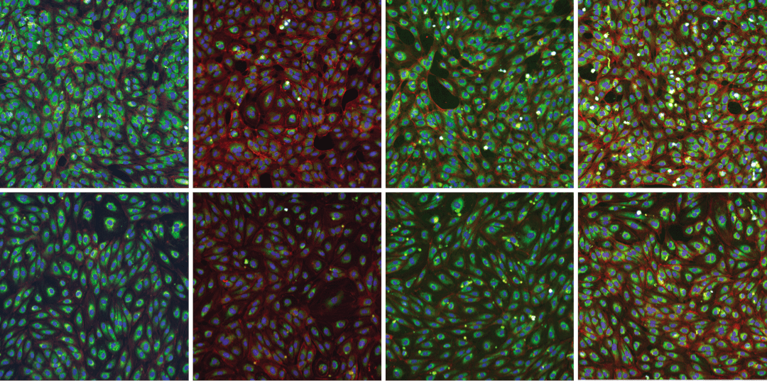"},{"metadata":{},"cell_type":"markdown","source":"
\n## [Competition Resources](https://www.kaggle.com/c/recursion-cellular-image-classification/overview/resources)\n## [RXRX](https://www.rxrx.ai/)\n## [Tutorials](https://github.com/recursionpharma/rxrx1-utils)"},{"metadata":{},"cell_type":"markdown","source":"
\n# How to visualize images in RxRx1\n\nThe RxRx1 cellular image dataset is made up of 6-channel images, where each channel illuminates different parts of the cell (visit [RxRx.ai](https://www.rxrx.ai/) for details). This notebook demonstrates how to use the code in [rxrx1-utils](https://github.com/recursionpharma/rxrx1-utils) to load and visualize the RxRx1 images."},{"metadata":{"_cell_guid":"79c7e3d0-c299-4dcb-8224-4455121ee9b0","_uuid":"d629ff2d2480ee46fbb7e2d37f6b5fab8052498a","trusted":true},"cell_type":"code","source":"import numpy as np # linear algebra\nimport pandas as pd # data processing, CSV file I/O (e.g. pd.read_csv)\nimport os\nprint(os.listdir(\"../input\"))\nimport sys\nimport matplotlib.pyplot as plt\n%matplotlib inline","execution_count":null,"outputs":[]},{"metadata":{"_kg_hide-output":false,"trusted":true},"cell_type":"code","source":"!git clone https://github.com/recursionpharma/rxrx1-utils\nprint ('rxrx1-utils cloned!')","execution_count":null,"outputs":[]},{"metadata":{"trusted":true},"cell_type":"code","source":"!ls","execution_count":null,"outputs":[]},{"metadata":{"trusted":true},"cell_type":"code","source":"sys.path.append('rxrx1-utils')\nimport rxrx.io as rio","execution_count":null,"outputs":[]},{"metadata":{},"cell_type":"markdown","source":"# Loading a site and visualizing individual channels\n\nUse load_site to get the 512 x 512 x 6 image tensor for a site. The arguments you pass to load_site tell it which image you want. In the example below, from the train set, we request the image in experiment RPE-05 on plate 3 in well D19 at site 2."},{"metadata":{"trusted":true},"cell_type":"code","source":"t = rio.load_site('train', 'RPE-05', 3, 'D19', 2)\nt.shape","execution_count":null,"outputs":[]},{"metadata":{},"cell_type":"markdown","source":"At this point, you can visualize the individual channels."},{"metadata":{"trusted":true},"cell_type":"code","source":"fig, axes = plt.subplots(2, 3, figsize=(24, 16))\n\nfor i, ax in enumerate(axes.flatten()):\n ax.axis('off')\n ax.set_title('channel {}'.format(i + 1))\n _ = ax.imshow(t[:, :, i], cmap='gray')","execution_count":null,"outputs":[]},{"metadata":{},"cell_type":"markdown","source":"The function load_site takes an optional base_path argument that defaults to *gs://rxrx1-us-central1/images*, one of the two Google Cloud Storage buckets containing the RxRx1 image set. You can also set base_path to the path of your local copy of the dataset, and this is how you'll typically want to work with this function."},{"metadata":{},"cell_type":"markdown","source":"# Converting a site to RGB format\n\nIn order to visualize all six channels at once, use **convert_tensor_to_rgb**. It associates an RGB color with each channel, then aggregates the color channels across the six cellular channels.\n\n"},{"metadata":{"trusted":true},"cell_type":"code","source":"x = rio.convert_tensor_to_rgb(t)\nx.shape","execution_count":null,"outputs":[]},{"metadata":{},"cell_type":"markdown","source":"Now plot your RGB image."},{"metadata":{"trusted":true},"cell_type":"code","source":"plt.figure(figsize=(8, 8))\nplt.axis('off')\n\n_ = plt.imshow(x)","execution_count":null,"outputs":[]},{"metadata":{},"cell_type":"markdown","source":"# Load and convert to RGB\nFor convenience, there is a wrapper around these two functions called ```load_site_as_rgb``` with the same signature as ```load_site```."},{"metadata":{"trusted":true},"cell_type":"code","source":"y = rio.load_site_as_rgb('train', 'HUVEC-08', 4, 'K09', 1)\n\nplt.figure(figsize=(8, 8))\nplt.axis('off')\n\n_ = plt.imshow(y)","execution_count":null,"outputs":[]},{"metadata":{},"cell_type":"markdown","source":"Beautiful images, aren't they?"},{"metadata":{},"cell_type":"markdown","source":"# Combining competition metadata\nThe metadata for RxRx1 during the Kaggle competition is broken up into four files: \n- ```train.csv```\n- ```train_controls.csv```\n- ```test.csv```\n- ```test_controls.csv```. \n\nIt is often more convenient to view all the metadata at once, so we have provided a helper function called combine_metadata for doing just that."},{"metadata":{"trusted":true},"cell_type":"code","source":"md = rio.combine_metadata()\nmd.head()","execution_count":null,"outputs":[]},{"metadata":{},"cell_type":"markdown","source":"The combined metadata adds a ```cell_type``` and dataset column, and specifies a well_type of \"treament\" for all non-control sirna. Note that the sirna column has **NaNs** for the non-control test images since those labels are not available during the competition (they are from the wells that need to be predicted), which forces the sirna column to be of type float."},{"metadata":{},"cell_type":"markdown","source":"# EDA"},{"metadata":{},"cell_type":"markdown","source":"### File Description\n- **[train/test].zip:** the image data. The image paths, such as ```U2OS-01/Plate1/B02_s2_w3.png```, can be read as:\n\n - Cell line and batch number (U2OS batch 1)\n - Plate number (1)\n - Well location on plate (column B, row 2)\n - Site (2)\n - Microscope channel (3)\n\nPlease note that the **[train/test].csv** and **[train/test]_controls.csv** combined describe the images found in **[train/test].zip.** You will only be making predictions on the images listed in **test.csv**, not on all the images found in **test.zip**.\n\n- **[train/test].csv**\n - id_code\n - experiment: the cell type and batch number\n - plate: plate number within the experiment\n - well: location on the plate\n - sirna: the target\n\n- **[train/test]_controls.csv** In each experiment, the same 30 siRNAs appear on every plate as positive controls. In addition, there is one well per plate with untreated cells as a negative control. It has the same schema as **[train/test].csv**, plus a ```well_type``` field denoting the type of control.\n\n**pixel_stats.csv** Provides the mean, standard deviation, median, min, and max pixel values for each channel of each image.\n**sample_submission.csv** A valid sample submission."},{"metadata":{"trusted":true},"cell_type":"code","source":"import seaborn as sns","execution_count":null,"outputs":[]},{"metadata":{"trusted":true},"cell_type":"code","source":"md.head(10)","execution_count":null,"outputs":[]},{"metadata":{"trusted":true},"cell_type":"code","source":"md.index","execution_count":null,"outputs":[]},{"metadata":{},"cell_type":"markdown","source":"### Unique values"},{"metadata":{"_kg_hide-input":true,"trusted":true},"cell_type":"code","source":"for i in md.columns:\n print (\">> \",i,\"\\t\", md[i].unique())","execution_count":null,"outputs":[]},{"metadata":{"_kg_hide-input":true,"trusted":true},"cell_type":"code","source":"for col in ['cell_type', 'dataset', 'experiment', 'plate', 'site', 'well_type']:\n print (col)\n print (md[col].value_counts())\n sns.countplot(y = col,\n data = md,\n order = md[col].value_counts().index)\n plt.show()\n ","execution_count":null,"outputs":[]},{"metadata":{},"cell_type":"markdown","source":"### Missing"},{"metadata":{"trusted":true},"cell_type":"code","source":"missing_values_count = md.isnull().sum()\nmissing_values_count","execution_count":null,"outputs":[]},{"metadata":{"trusted":true},"cell_type":"code","source":"md = md.fillna(0)\nmd.head()","execution_count":null,"outputs":[]},{"metadata":{},"cell_type":"markdown","source":"### sirna distribution"},{"metadata":{"trusted":true},"cell_type":"code","source":"train_df = md[md['dataset'] == 'train']\ntest_df = md[md['dataset'] == 'test']\n\ntrain_df.shape, test_df.shape","execution_count":null,"outputs":[]},{"metadata":{"trusted":true},"cell_type":"code","source":"plt.figure(figsize=(16,6))\nplt.title(\"Distribution of SIRNA in the train and test set\")\nsns.distplot(train_df.sirna,color=\"green\", kde=True,bins='auto', label='train')\nsns.distplot(test_df.sirna,color=\"blue\", kde=True, bins='auto', label='test')\nplt.legend()\nplt.show()","execution_count":null,"outputs":[]},{"metadata":{},"cell_type":"markdown","source":"Remember, 0s were NaNs"},{"metadata":{"trusted":true},"cell_type":"code","source":"feat1 = 'sirna'\nfig = plt.subplots(figsize=(15, 5))\n\n# train\nplt.subplot(1, 2, 1)\nsns.kdeplot(train_df[feat1][train_df['site'] == 1], shade=False, color=\"b\", label = 'site 1')\nsns.kdeplot(train_df[feat1][train_df['site'] == 2], shade=False, color=\"r\", label = 'site 2')\nplt.title(feat1)\nplt.xlabel('Feature Values')\nplt.ylabel('Probability')\n\n# test\nplt.subplot(1, 2, 2)\nsns.kdeplot(test_df[feat1][test_df['site'] == 1], shade=False, color=\"b\", label = 'site 1')\nsns.kdeplot(test_df[feat1][test_df['site'] == 2], shade=False, color=\"r\", label = 'site 2')\nplt.title(feat1)\nplt.xlabel('Feature Values')\nplt.ylabel('Probability')\nplt.show()","execution_count":null,"outputs":[]},{"metadata":{"trusted":true},"cell_type":"code","source":"","execution_count":null,"outputs":[]},{"metadata":{"trusted":true},"cell_type":"code","source":"# Prevent: Output path '/rxrx1-utils/.git/logs/refs/remotes/origin/HEAD' contains too many nested subdirectories (max 6)\n!rm -r rxrx1-utils\n!ls","execution_count":null,"outputs":[]},{"metadata":{},"cell_type":"markdown","source":"# To Be Continued ..."}],"metadata":{"kernelspec":{"display_name":"Python 3","language":"python","name":"python3"},"language_info":{"name":"python","version":"3.6.4","mimetype":"text/x-python","codemirror_mode":{"name":"ipython","version":3},"pygments_lexer":"ipython3","nbconvert_exporter":"python","file_extension":".py"}},"nbformat":4,"nbformat_minor":1}