\n### 2-3-1 Data fields\n1. qid - unique question identifier\n1. question_text - Quora question text\n1. target - a question labeled \"insincere\" has a value of 1, otherwise 0"},{"metadata":{"trusted":true,"_uuid":"25e57422e63164b80709d9352866f59a8264d29d"},"cell_type":"code","source":"train = pd.read_csv('../input/train.csv')\ntest = pd.read_csv('../input/test.csv')","execution_count":null,"outputs":[]},{"metadata":{"trusted":true,"_uuid":"e11494ec5201b90e5c404b6f9d27877d8e866f3a"},"cell_type":"code","source":"type(train)","execution_count":null,"outputs":[]},{"metadata":{"_uuid":"64c63d1c4b687c90b96a8f5218aa3a17ddf756d1"},"cell_type":"markdown","source":"To check the first 5 rows of the data set, we can use head(5)."},{"metadata":{"trusted":true,"_uuid":"3480a17f080f98ff7a2b168da5b5b51893c881b4"},"cell_type":"code","source":"train.head(5) ","execution_count":null,"outputs":[]},{"metadata":{"_uuid":"d3e463743678b24042db613aa689f5e2d5aef0db"},"cell_type":"markdown","source":"
\n### 2-3-2 Target\nYou will be predicting whether a question asked on **Quora** is sincere or not."},{"metadata":{"_uuid":"54c2884d6777cac8a94d034ad1d112a3ffab4ca0"},"cell_type":"markdown","source":"
\n## 2-4 EDA\nIn this section, you'll learn how to use graphical and numerical techniques to begin uncovering the structure of your data.\n1. Which variables suggest interesting relationships?\n1. Which observations are unusual?\n1. Analysis of the features! By the end of the section, you'll be able to answer these questions and more, while generating. "},{"metadata":{"trusted":true,"_uuid":"57c67feb26a1c058151facc84145339f8bc89cfc","_kg_hide-input":true},"cell_type":"code","source":"train.sample(5)","execution_count":null,"outputs":[]},{"metadata":{"_uuid":"40a7cd1995977c500bcfd47e2b792cd8d6f9ae92"},"cell_type":"markdown","source":"To pop up 5 random rows from the data set, we can use **sample(5**) function."},{"metadata":{"trusted":true,"_uuid":"9d26d55e5ea4ff0255499c3bba01940a73a116f7","_kg_hide-input":true},"cell_type":"code","source":"test.sample(5)","execution_count":null,"outputs":[]},{"metadata":{"_uuid":"1079234af07e56378d1c436a2f3127ccd4ecaec8"},"cell_type":"markdown","source":"To check out last 5 row of the data set, we use tail() function."},{"metadata":{"trusted":true,"_uuid":"986660265598c78d177d6b1028abaa9e4bbf0d56","_kg_hide-input":true},"cell_type":"code","source":"train.tail()","execution_count":null,"outputs":[]},{"metadata":{"trusted":true,"_uuid":"744f1cc507d8fec6ca85d2d36c5ae85a2cd7237a"},"cell_type":"code","source":"print(train.shape)\nprint(test.shape)","execution_count":null,"outputs":[]},{"metadata":{"_uuid":"5bf7fbd5cc4a2118740c30436eed151dc10f579a"},"cell_type":"markdown","source":"To check out how many null info are on the dataset, we can use **isnull().sum()**."},{"metadata":{"trusted":true,"_uuid":"ca2228b14d432b7e6e3a66babc6a8c292ca72fbf","_kg_hide-input":true},"cell_type":"code","source":"train.isnull().sum()","execution_count":null,"outputs":[]},{"metadata":{"trusted":true,"_uuid":"b956b1a917722a01b06135be457b92f4e226243a","_kg_hide-input":true},"cell_type":"code","source":"test.isnull().sum()","execution_count":null,"outputs":[]},{"metadata":{"_uuid":"61a7dea9e3435ac6ef19935621af5baf33c6124e"},"cell_type":"markdown","source":"### 2-4-1 About Quora\nQuora is a platform that empowers people to learn from each other. On Quora, people can ask questions and connect with others who contribute unique insights and quality answers. A key challenge is to weed out insincere questions -- those founded upon false premises, or that intend to make a statement rather than look for helpful answers."},{"metadata":{"trusted":true,"_uuid":"468755c147347cfea72cc9cf21e50541a55d347e","_kg_hide-input":true},"cell_type":"code","source":"print(train.info())","execution_count":null,"outputs":[]},{"metadata":{"_uuid":"8e4f6d001e1c959f034a0497c09fb18b309b2816"},"cell_type":"markdown","source":"to give a statistical summary about the dataset, we can use **describe()**."},{"metadata":{"trusted":true,"_uuid":"a242adcee764b28ed57f49111a5b94c1a19ba9f0","_kg_hide-input":true},"cell_type":"code","source":"train.describe() ","execution_count":null,"outputs":[]},{"metadata":{"_uuid":"bca11ce44f7ebdd1de3868fb2f6c50b0e7c7cb16"},"cell_type":"markdown","source":"###### [Go to top](#top)"},{"metadata":{"_uuid":"2d96fedf1a2fa6344990cb07b8d98d17a3a7b504"},"cell_type":"markdown","source":"
\n# 3- Python Deep Learning Packages\n
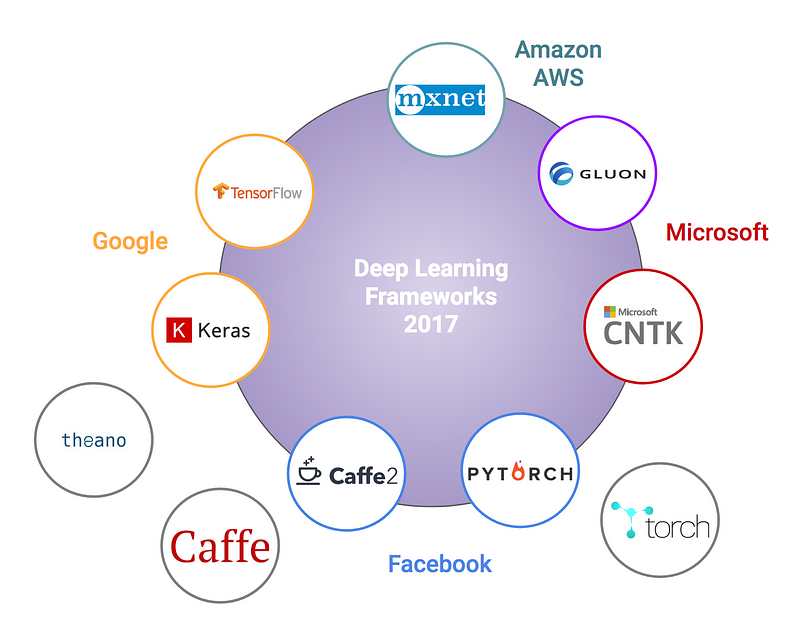 \n*State of open source deep learning frameworks in 2017* [**towardsdatascience**](https://towardsdatascience.com/battle-of-the-deep-learning-frameworks-part-i-cff0e3841750)\n1. **keras**[11]\n>Well known for being minimalistic, the Keras neural network library (with a supporting interface of Python) supports both convolutional and recurrent networks that are capable of running on either TensorFlow or Theano. The library is written in Python and was developed keeping quick experimentation as its USP.\n1. **TensorFlow**\n> TensorFlow is arguably one of the best deep learning frameworks and has been adopted by several giants such as Airbus, Twitter, IBM, and others mainly due to its highly flexible system architecture.\n1. **Caffe**\n> Caffe is a deep learning framework that is supported with interfaces like C, C++, Python, and MATLAB as well as the command line interface. It is well known for its speed and transposability and its applicability in modeling convolution neural networks (CNN).\n1. **Microsoft Cognitive Toolkit/CNTK**\n> Popularly known for easy training and the combination of popular model types across servers, the Microsoft Cognitive Toolkit (previously known as CNTK) is an open-source deep learning framework to train deep learning models. It performs efficient convolution neural networks and training for image, speech, and text-based data. Similar to Caffe, it is supported by interfaces such as Python, C++, and the command line interface.\n1. **Torch/PyTorch**\n> Torch is a scientific computing framework that offers wide support for machine learning algorithms. It is a Lua-based deep learning framework and is used widely amongst industry giants such as Facebook, Twitter, and Google. It employs CUDA along with C/C++ libraries for processing and was basically made to scale the production of building models and provide overall flexibility.\n1. **MXNet**\n> Designed specifically for the purpose of high efficiency, productivity, and flexibility, MXNet(pronounced as mix-net) is a deep learning framework supported by Python, R, C++, and Julia.\n1. **Chainer**\n>Highly powerful, dynamic and intuitive, Chainer is a Python-based deep learning framework for neural networks that is designed by the run strategy. Compared to other frameworks that use the same strategy, you can modify the networks during runtime, allowing you to execute arbitrary control flow statements.\n1. **Deeplearning4j**\n>Parallel training through iterative reduce, microservice architecture adaptation, and distributed CPUs and GPUs are some of the salient features of the Deeplearning4j deep learning framework. It is developed in Java as well as Scala and supports other JVM languages, too.\n1. **Theano**\n>Theano is beautiful. Without Theano, we wouldn’t have anywhere near the amount of deep learning libraries (specifically in Python) that we do today. In the same way that without NumPy, we couldn’t have SciPy, scikit-learn, and scikit-image, the same can be said about Theano and higher-level abstractions of deep learning.\n1. **Lasagne**\n>Lasagne is a lightweight library used to construct and train networks in Theano. The key term here is lightweight — it is not meant to be a heavy wrapper around Theano like Keras is. While this leads to your code being more verbose, it does free you from any restraints, while still giving you modular building blocks based on Theano.\n1. **PaddlePaddle**\n>PaddlePaddle (PArallel Distributed Deep LEarning) is an easy-to-use, efficient, flexible and scalable deep learning platform, which is originally developed by Baidu scientists and engineers for the purpose of applying deep learning to many products at Baidu.\n\n###### [Go to top](#top)"},{"metadata":{"_uuid":"0560fa84a64ddeac53a4a10aaaa04a1424ad50f9"},"cell_type":"markdown","source":"
 \n# 4- Frameworks - We will look at TensorFlow and Keras.\nLet's Start Learning, in this section we intrduce 5 deep learning frameworks."},{"metadata":{"_uuid":"cc17ec452b22997c92948c59852e319960f8de48"},"cell_type":"markdown","source":"
\n## 4-1 Keras\nOur workflow will be as follow[10] [deep-learning-with-python-notebooks](https://github.com/fchollet/deep-learning-with-python-notebooks):\n1. first we will present our neural network with the training data, `train_images` and `train_labels`. \n1. The network will then learn to associate images and labels. \n1. Finally, we will ask the network to produce predictions for `test_images`, \n1. and we will verify if these predictions match the labels from `test_labels`.\n\n**Let's build our network **\n\n###### [Go to top](#top)"},{"metadata":{"trusted":true,"_uuid":"c1d0fd821b1058f2f0f3a60bca814a199472bab8","_kg_hide-input":true},"cell_type":"code","source":"# import Dataset to play with it\nfrom keras.datasets import mnist\n\n(train_images, train_labels), (test_images, test_labels) = mnist.load_data()","execution_count":null,"outputs":[]},{"metadata":{"_kg_hide-input":true,"_uuid":"372dc6b32cdfdd8cdcec96ecd7589c6c2b8f857d","trusted":true},"cell_type":"code","source":"from keras import models\nfrom keras import layers\n\nnetwork = models.Sequential()\nnetwork.add(layers.Dense(512, activation='relu', input_shape=(28 * 28,)))\nnetwork.add(layers.Dense(10, activation='softmax'))","execution_count":null,"outputs":[]},{"metadata":{"_uuid":"bb4af579abbb2d8de84c8799bbca2a9129166b75"},"cell_type":"markdown","source":"
\n## 4-1-1 Analysis\nThe core building block of neural networks is the \"**layer**\", a data-processing module which you can conceive as a \"**filter**\" for data. Some data comes in, and comes out in a more useful form. Precisely, layers extract _representations_ out of the data fed into them -- hopefully representations that are more meaningful for the problem at hand. Most of deep learning really consists of chaining together simple layers which will implement a form of progressive \"**data distillation**\". [colab.research.google](https://colab.research.google.com/github/alzayats/Google_Colab/blob/master/2_1_a_first_look_at_a_neural_network.ipynb)\nA deep learning model is like a sieve for data processing, made of a succession of increasingly refined data filters -- the \"layers\".\nHere our network consists of a sequence of two `Dense` layers, which are densely-connected (also called \"fully-connected\") neural layers. \nThe second (and last) layer is a 10-way \"**softmax**\" layer, which means it will return an array of 10 probability scores (summing to 1). Each score will be the probability that the current digit image belongs to one of our 10 digit classes.\nTo make our network ready for training, we need to pick three more things, as part of \"compilation\" step:\n\n1. A loss function: the is how the network will be able to measure how good a job it is doing on its training data, and thus how it will be able to steer itself in the right direction.\n1. An optimizer: this is the mechanism through which the network will update itself based on the data it sees and its loss function.\n1. Metrics to monitor during training and testing. Here we will only care about accuracy (the fraction of the images that were correctly classified).\n\n###### [Go to top](#top)"},{"metadata":{"_kg_hide-input":true,"_uuid":"f1c5dde77030c5917a6192452a9b27d93aafc04f","trusted":true},"cell_type":"code","source":"network.compile(optimizer='rmsprop',\n loss='categorical_crossentropy',\n metrics=['accuracy'])","execution_count":null,"outputs":[]},{"metadata":{"_uuid":"4512d98c72019135dd41f9f0521be6ece298be24"},"cell_type":"markdown","source":"\nBefore training, we will **preprocess** our data by reshaping it into the shape that the network expects, and **scaling** it so that all values are in \nthe `[0, 1]` interval. Previously, our training images for instance were stored in an array of shape `(60000, 28, 28)` of type `uint8` with \nvalues in the `[0, 255]` interval. We transform it into a `float32` array of shape `(60000, 28 * 28)` with values between 0 and 1.\n\n###### [Go to top](#top)"},{"metadata":{"_kg_hide-input":true,"_uuid":"11ab3b8562444b8af7c342c36a45fefa20387e3b","trusted":true},"cell_type":"code","source":"train_images = train_images.reshape((60000, 28 * 28))\ntrain_images = train_images.astype('float32') / 255\n\ntest_images = test_images.reshape((10000, 28 * 28))\ntest_images = test_images.astype('float32') / 255","execution_count":null,"outputs":[]},{"metadata":{"_uuid":"ff688de9ee4e5ec11da63bb2f3ef48a49d7b2dd7"},"cell_type":"markdown","source":"We also need to **categorically encode** the labels"},{"metadata":{"_kg_hide-input":true,"_uuid":"fc813e561b55b29d1e0ba7f620ae29bf43293b57","trusted":true},"cell_type":"code","source":"from keras.utils import to_categorical\n\ntrain_labels = to_categorical(train_labels)\ntest_labels = to_categorical(test_labels)","execution_count":null,"outputs":[]},{"metadata":{"_uuid":"fe77d9bdd7566b201e5be7fe54c67c7f9717c956"},"cell_type":"markdown","source":"We are now ready to train our network, which in **Keras** is done via a call to the `fit` method of the network: \nwe \"fit\" the model to its training data.\n\n###### [Go to top](#top)"},{"metadata":{"_uuid":"18dd966ba9e372810d2e6ef3950182a6fb91f779","trusted":true,"_kg_hide-input":true},"cell_type":"code","source":"#please change epochs to 5\nnetwork.fit(train_images, train_labels, epochs=1, batch_size=128)","execution_count":null,"outputs":[]},{"metadata":{"_uuid":"7542f033cbc2c6a14b406319e822b2482600bc55"},"cell_type":"markdown","source":"**Two quantities** are being displayed during training: the \"**loss**\" of the network over the training data, and the accuracy of the network over \nthe training data.\n\nWe quickly reach an accuracy of **0.989 (i.e. 98.9%)** on the training data. Now let's check that our model performs well on the test set too:\n\n###### [Go to top](#top)"},{"metadata":{"_uuid":"b3ed834610a6f66f1e112a7c8288e84a0dd410b8","trusted":true,"_kg_hide-input":true},"cell_type":"code","source":"test_loss, test_acc = network.evaluate(test_images, test_labels)","execution_count":null,"outputs":[]},{"metadata":{"_uuid":"0e00d4ca1dff83c73886044b8049d4fcc6930669","trusted":true,"_kg_hide-input":true},"cell_type":"code","source":"print('test_acc:', test_acc)","execution_count":null,"outputs":[]},{"metadata":{"_uuid":"ac27321f82907d98f22b2ab6fee54a5885c7cbb1"},"cell_type":"markdown","source":"\n**Our test set accuracy turns out to be 97.8%**"},{"metadata":{"_uuid":"938b17914c9b6249a82dd3d8063d77511ec1ac5b"},"cell_type":"markdown","source":"
\n## 4-1-2 Text Classification with Keras\nA simple text classification from [16]."},{"metadata":{"trusted":true,"_uuid":"64017109bf27fb614934740111e705cae904ed13"},"cell_type":"code","source":"from keras.preprocessing import sequence\nfrom keras.models import Sequential\nfrom keras.layers import Dense, Embedding, GlobalAveragePooling1D\nfrom keras.datasets import imdb","execution_count":null,"outputs":[]},{"metadata":{"_uuid":"2d318a6552c109d8880ce14659c90210eab060c0"},"cell_type":"markdown","source":"
\n## 4-2 TensorFlow\n**TensorFlow** is an open-source machine learning library for research and production. TensorFlow offers **APIs** for beginners and experts to develop for desktop, mobile, web, and cloud. See the sections below to get started.[12] [tensorflow](https://www.tensorflow.org/tutorials)\n\n###### [Go to top](#top)"},{"metadata":{"_kg_hide-input":true,"_uuid":"e5f85da49eb80ae47151b5b3308425b9184e1440","trusted":true},"cell_type":"code","source":"# Simple hello world using TensorFlow\nhello = tf.constant('Hello, TensorFlow!')\n# Start tf session\nsess = tf.Session()\n# Run graph\nprint(sess.run(hello))\nmnist = tf.keras.datasets.mnist\n\n(x_train, y_train),(x_test, y_test) = mnist.load_data()\nx_train, x_test = x_train / 255.0, x_test / 255.0\n\nmodel = tf.keras.models.Sequential([\n tf.keras.layers.Flatten(),\n tf.keras.layers.Dense(512, activation=tf.nn.relu),\n tf.keras.layers.Dropout(0.2),\n tf.keras.layers.Dense(10, activation=tf.nn.softmax)\n])\nmodel.compile(optimizer='adam',\n loss='sparse_categorical_crossentropy',\n metrics=['accuracy'])\n#please change epochs to 5\nmodel.fit(x_train, y_train, epochs=1)\nmodel.evaluate(x_test, y_test)","execution_count":null,"outputs":[]},{"metadata":{"_uuid":"fbc9fbb67e838ea9ddf88845b688c8c1951f7512"},"cell_type":"markdown","source":"
\n## 4-2-1 Import the Fashion MNIST dataset\n"},{"metadata":{"_uuid":"c85ca45a881ec8f85cf072cd8cc299e540e0b453","trusted":true,"_kg_hide-input":true},"cell_type":"code","source":"fashion_mnist = keras.datasets.fashion_mnist\n\n(train_images, train_labels), (test_images, test_labels) = fashion_mnist.load_data()","execution_count":null,"outputs":[]},{"metadata":{"_uuid":"06829a241c328ba053315979757694774808e3c0"},"cell_type":"markdown","source":"Loading the dataset returns **four NumPy arrays**:\n\n1. The train_images and train_labels arrays are the training set—the data the model uses to learn.\n1. The model is tested against the test set, the test_images, and test_labels arrays.\n1. The images are 28x28 NumPy arrays, with pixel values ranging between 0 and 255.\n1. The labels are an array of integers, ranging from 0 to 9. These correspond to the class of clothing the image represents:\n\n###### [Go to top](#top)"},{"metadata":{"_uuid":"ed1e9b140ee497c89ac5213787c157d412385ac6"},"cell_type":"markdown","source":"
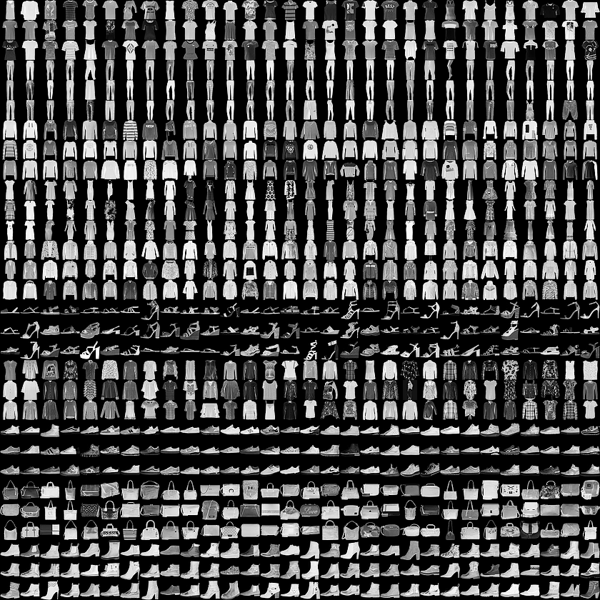 \n[image credit](https://tensorflow.org)"},{"metadata":{"_uuid":"302664d8f9878c0c8ddb2a64bc00cd6ed58d4766"},"cell_type":"markdown","source":"Each image is **mapped** to a single label. Since the class names are not included with the dataset, store them here to use later when plotting the images:"},{"metadata":{"_uuid":"0801170ba61fca12c2d39f246bcb4ece5f78f5df","trusted":true,"_kg_hide-input":true},"cell_type":"code","source":"class_names = ['T-shirt/top', 'Trouser', 'Pullover', 'Dress', 'Coat', \n 'Sandal', 'Shirt', 'Sneaker', 'Bag', 'Ankle boot']","execution_count":null,"outputs":[]},{"metadata":{"_uuid":"f2136d7bc6f8ef021e4d7f6ee69203baf43faabd"},"cell_type":"markdown","source":"
 \n## 4-2-2 Explore the data\nLet's explore the format of the dataset before training the model. The following shows there are **60,000** images in the training set, with each image represented as 28 x 28 pixels:\n\n###### [Go to top](#top)"},{"metadata":{"_uuid":"1f4dc17d2affe5849b9a4e8ae81d2c9ffa5739c9","trusted":true,"_kg_hide-input":true},"cell_type":"code","source":"train_images.shape","execution_count":null,"outputs":[]},{"metadata":{"_uuid":"9cbf875d1bb38ca779bf1ea9d081887889b18206"},"cell_type":"markdown","source":"Likewise, there are 60,000 labels in the training set:\n\n"},{"metadata":{"_uuid":"8dc01e76b4d061bacbfaca818dac4ac6f15c7a44","trusted":true,"_kg_hide-input":true},"cell_type":"code","source":"len(train_labels)","execution_count":null,"outputs":[]},{"metadata":{"_uuid":"dac4b85e6bbe9c6909ccaad22dfba927d8a95fe4"},"cell_type":"markdown","source":"Each label is an integer between 0 and 9:\n\n"},{"metadata":{"_uuid":"9b1060a16ba153a47f8f9576281934d570b76a2b","trusted":true,"_kg_hide-input":true},"cell_type":"code","source":"train_labels","execution_count":null,"outputs":[]},{"metadata":{"_uuid":"6b9524c3d082ba3d1fe08fc5117350d3831720ce"},"cell_type":"markdown","source":"There are 10,000 images in the test set. Again, each image is represented as 28 x 28 pixels:\n\n"},{"metadata":{"_uuid":"11acf0145fd4293e8944da17db96ef0abf176fe2","trusted":true,"_kg_hide-input":true},"cell_type":"code","source":"test_images.shape","execution_count":null,"outputs":[]},{"metadata":{"_uuid":"10d203635805eb675a08a1aa6cac8a18198bddb0"},"cell_type":"markdown","source":"And the test set contains 10,000 images labels:\n\n"},{"metadata":{"_uuid":"fa2d61fe145d2040832162e2ab1cb42edb7aa3d1","trusted":true,"_kg_hide-input":true},"cell_type":"code","source":"len(test_labels)","execution_count":null,"outputs":[]},{"metadata":{"_uuid":"aba35c08f64f4879210aaf6c8954e361cc34a6fb"},"cell_type":"markdown","source":"
\n## 4-2-3 Preprocess the data\n"},{"metadata":{"_uuid":"3d2f80c0d183ef02499dfba9e1d91e98aa109ada"},"cell_type":"markdown","source":"The data must be preprocessed before training the network. If you inspect the first image in the training set, you will see that the pixel values fall in the range of 0 to 255:\n\n###### [Go to top](#top)\n"},{"metadata":{"_uuid":"45f0894f5fbb16cfb153ab368db499f5ca3bf898","trusted":true,"_kg_hide-input":true},"cell_type":"code","source":"plt.figure()\nplt.imshow(train_images[0])\nplt.colorbar()\nplt.grid(False)","execution_count":null,"outputs":[]},{"metadata":{"_uuid":"d9d3aa056608f5ba327ade5a012a5732aa588a58"},"cell_type":"markdown","source":"We scale these values to a range of 0 to 1 before feeding to the neural network model. For this, cast the datatype of the image components from an** integer to a float,** and divide by 255. Here's the function to preprocess the images:\n\nIt's important that the training set and the testing set are preprocessed in the same way:"},{"metadata":{"_uuid":"00845f727dea68873dd406f5eb70f4f6b47f8109","trusted":true,"_kg_hide-input":true},"cell_type":"code","source":"train_images = train_images / 255.0\n\ntest_images = test_images / 255.0","execution_count":null,"outputs":[]},{"metadata":{"_uuid":"986c4006f09b115a8406c20f56b471ff99a77b7b"},"cell_type":"markdown","source":"Display the first 25 images from the training set and display the class name below each image. **Verify** that the data is in the correct format and we're ready to build and train the network."},{"metadata":{"_uuid":"741d898b017fcbf4cda5f1db742cd9a0f88b4edd","trusted":true,"_kg_hide-input":true},"cell_type":"code","source":"plt.figure(figsize=(10,10))\nfor i in range(25):\n plt.subplot(5,5,i+1)\n plt.xticks([])\n plt.yticks([])\n plt.grid(False)\n plt.imshow(train_images[i], cmap=plt.cm.binary)\n plt.xlabel(class_names[train_labels[i]])","execution_count":null,"outputs":[]},{"metadata":{"_uuid":"2097815c69672cd1b9f56448acdf437339f568c9"},"cell_type":"markdown","source":"
\n## 4-2-4 Build the model\n"},{"metadata":{"_uuid":"d7b5a268f8e1dc866e7a3fb3a2f6cca0e8523240"},"cell_type":"markdown","source":"**Building the neural network requires configuring the layers of the model, then compiling the model.**\n
\n### 4-2-4-1 Setup the layers\nThe basic building block of a neural network is the layer. **Layers** extract representations from the data fed into them. And, hopefully, these representations are more meaningful for the problem at hand.\n\nMost of deep learning consists of chaining together simple layers. Most layers, like tf.keras.layers.Dense, have parameters that are learned during training.\n\n###### [Go to top](#top)"},{"metadata":{"_kg_hide-input":true,"_uuid":"2fb66496035a544a5e94106cb2b80e7bcb11d5d4","trusted":true},"cell_type":"code","source":"model = keras.Sequential([\n keras.layers.Flatten(input_shape=(28, 28)),\n keras.layers.Dense(128, activation=tf.nn.relu),\n keras.layers.Dense(10, activation=tf.nn.softmax)\n])","execution_count":null,"outputs":[]},{"metadata":{"_uuid":"891b791c682f6512cb837e4c9cd3bb3f96f255f7"},"cell_type":"markdown","source":"The **first layer** in this network, tf.keras.layers.Flatten, transforms the format of the images from a 2d-array (of 28 by 28 pixels), to a 1d-array of 28 * 28 = 784 pixels. Think of this layer as unstacking rows of pixels in the image and lining them up. This layer has no parameters to learn; it only reformats the data.\n\nAfter the pixels are flattened, the network consists of a sequence of two tf.keras.layers.Dense layers. These are densely-connected, or fully-connected, neural layers. The first Dense layer has 128 nodes (or neurons). **The second (and last) layer** is a 10-node softmax layer—this returns an array of 10 probability scores that sum to 1. Each node contains a score that indicates the probability that the current image belongs to one of the 10 classes.\n\n###### [Go to top](#top)"},{"metadata":{"_uuid":"b8288c8b9365aaea1be7e3fc29f28ea099599337"},"cell_type":"markdown","source":"
\n## 4-2-5 Compile the model\nBefore the model is ready for training, it needs a few more settings. These are added during the model's compile step:\n\n1. **Loss function** —This measures how accurate the model is during training. We want to minimize this function to \"steer\" the model in the right direction.\n1. **Optimizer** —This is how the model is updated based on the data it sees and its loss function.\n1. **Metrics** —Used to monitor the training and testing steps. The following example uses accuracy, the fraction of the images that are correctly classified.\n\n###### [Go to top](#top)"},{"metadata":{"_kg_hide-input":true,"_uuid":"147f6384ab4ac6ca1f4199c9e5fe5fc5de40ddcf","trusted":true},"cell_type":"code","source":"model.compile(optimizer=tf.train.AdamOptimizer(), \n loss='sparse_categorical_crossentropy',\n metrics=['accuracy'])","execution_count":null,"outputs":[]},{"metadata":{"_uuid":"eb5ca06622460737f9270c0f8b44e4a9ec8ee46c"},"cell_type":"markdown","source":"
\n## 4-2-6 Train the model\nTraining the neural network model requires the following steps:\n\nFeed the training data to the model—in this example, the train_images and train_labels arrays.\nThe model learns to associate images and labels.\nWe ask the model to make predictions about a test set—in this example, the test_images array. We verify that the predictions match the labels from the test_labels array.\nTo start training, call the model.fit method—the model is \"fit\" to the training data:\n\n###### [Go to top](#top)"},{"metadata":{"_uuid":"03987dc45cf8603ac85093b2e213b66414997307","trusted":true,"_kg_hide-input":true},"cell_type":"code","source":"#please change epochs to 5\nmodel.fit(train_images, train_labels, epochs=1)","execution_count":null,"outputs":[]},{"metadata":{"_uuid":"1ac81e58e42d648d321b830b224ab3519984ebf3"},"cell_type":"markdown","source":"As the model trains, the loss and accuracy metrics are displayed. This model reaches an accuracy of about 0.88 (or 88%) on the training data."},{"metadata":{"_uuid":"87b748f0572109246d2867d3cbd0099279a8e14b"},"cell_type":"markdown","source":"
\n## 4-2-7 Evaluate accuracy\nNext, compare how the model performs on the test dataset:\n\n###### [Go to top](#top)"},{"metadata":{"_uuid":"6b058c57a1019bfe9eb5bb130821521b8fb60199","trusted":true,"_kg_hide-input":true},"cell_type":"code","source":"test_loss, test_acc = model.evaluate(test_images, test_labels)\n\nprint('Test accuracy:', test_acc)","execution_count":null,"outputs":[]},{"metadata":{"_uuid":"1e51ac16e784f873d188f3a7a9a97b77b80bc9fd"},"cell_type":"markdown","source":"It turns out, the accuracy on the test dataset is a little less than the accuracy on the training dataset. This gap between training accuracy and test accuracy is an example of overfitting. Overfitting is when a machine learning model performs worse on new data than on their training data."},{"metadata":{"_uuid":"89b4451f22b40620f84d91776bc87f56c7035b56"},"cell_type":"markdown","source":"
\n## 4-2-8 Make predictions\nWith the model trained, we can use it to make predictions about some images.\n###### [Go to top](#top)"},{"metadata":{"_uuid":"41c87068a6d3a43561ea86165f0a06a2118a62d2","trusted":true,"_kg_hide-input":true},"cell_type":"code","source":"predictions = model.predict(test_images)","execution_count":null,"outputs":[]},{"metadata":{"_uuid":"7c67111925e00718f02853fa0a2e075e57ca11a9"},"cell_type":"markdown","source":"Here, the model has predicted the label for each image in the testing set. Let's take a look at the first prediction:\n\n"},{"metadata":{"_uuid":"b55b3fd88dcc23ad88449a3e4031c8cafb898eb0","trusted":true,"_kg_hide-input":true},"cell_type":"code","source":"predictions[0]","execution_count":null,"outputs":[]},{"metadata":{"_uuid":"133bc34cbb4d3f253c524f00e222928a3b13e4b4"},"cell_type":"markdown","source":"A prediction is an array of 10 numbers. These describe the \"confidence\" of the model that the image corresponds to each of the 10 different articles of clothing. We can see which label has the highest confidence value:\n\n"},{"metadata":{"_uuid":"5d06c4e9c154f2a5b104fb40950caea662866928","trusted":true,"_kg_hide-input":true},"cell_type":"code","source":"np.argmax(predictions[0])","execution_count":null,"outputs":[]},{"metadata":{"_uuid":"416bd6ab38af768e7ccbf84f2e4958edf57607a7"},"cell_type":"markdown","source":"We can graph this to look at the full set of 10 channels\n\n"},{"metadata":{"_kg_hide-input":true,"_uuid":"f47aca692a640ad3b80f8866d6008aba68ed0825","trusted":true},"cell_type":"code","source":"def plot_image(i, predictions_array, true_label, img):\n predictions_array, true_label, img = predictions_array[i], true_label[i], img[i]\n plt.grid(False)\n plt.xticks([])\n plt.yticks([])\n \n plt.imshow(img, cmap=plt.cm.binary)\n\n predicted_label = np.argmax(predictions_array)\n if predicted_label == true_label:\n color = 'blue'\n else:\n color = 'red'\n \n plt.xlabel(\"{} {:2.0f}% ({})\".format(class_names[predicted_label],\n 100*np.max(predictions_array),\n class_names[true_label]),\n color=color)\n\ndef plot_value_array(i, predictions_array, true_label):\n predictions_array, true_label = predictions_array[i], true_label[i]\n plt.grid(False)\n plt.xticks([])\n plt.yticks([])\n thisplot = plt.bar(range(10), predictions_array, color=\"#777777\")\n plt.ylim([0, 1]) \n predicted_label = np.argmax(predictions_array)\n \n thisplot[predicted_label].set_color('red')\n thisplot[true_label].set_color('blue')","execution_count":null,"outputs":[]},{"metadata":{"_uuid":"659d69546cc3ba435b279de4b3672a73b4c188c2"},"cell_type":"markdown","source":"Let's look at the 0th image, predictions, and prediction array.\n\n###### [Go to top](#top)"},{"metadata":{"_uuid":"6567c22e4a9e6f5bb08971148ec301d7851293c1","trusted":true,"_kg_hide-input":true},"cell_type":"code","source":"i = 0\nplt.figure(figsize=(6,3))\nplt.subplot(1,2,1)\nplot_image(i, predictions, test_labels, test_images)\nplt.subplot(1,2,2)\nplot_value_array(i, predictions, test_labels)","execution_count":null,"outputs":[]},{"metadata":{"_uuid":"6d38e7cb0dafada9806aa9e97ea96b77f64c43da","trusted":true,"_kg_hide-input":true},"cell_type":"code","source":"i = 12\nplt.figure(figsize=(6,3))\nplt.subplot(1,2,1)\nplot_image(i, predictions, test_labels, test_images)\nplt.subplot(1,2,2)\nplot_value_array(i, predictions, test_labels)","execution_count":null,"outputs":[]},{"metadata":{"_uuid":"cb5e128f74d125f210335318f1caad4d9d57c93c"},"cell_type":"markdown","source":"Let's plot several images with their predictions. Correct prediction labels are blue and incorrect prediction labels are red. The number gives the percent (out of 100) for the predicted label. Note that it can be wrong even when very confident.\n\n###### [Go to top](#top)"},{"metadata":{"_uuid":"1bfd76dfc22dc76ccc17eaa2209144cb0571b0a4","trusted":true,"_kg_hide-input":true},"cell_type":"code","source":"# Plot the first X test images, their predicted label, and the true label\n# Color correct predictions in blue, incorrect predictions in red\nnum_rows = 5\nnum_cols = 3\nnum_images = num_rows*num_cols\nplt.figure(figsize=(2*2*num_cols, 2*num_rows))\nfor i in range(num_images):\n plt.subplot(num_rows, 2*num_cols, 2*i+1)\n plot_image(i, predictions, test_labels, test_images)\n plt.subplot(num_rows, 2*num_cols, 2*i+2)\n plot_value_array(i, predictions, test_labels)","execution_count":null,"outputs":[]},{"metadata":{"_uuid":"aad0da875f601a4834cb339909d54f5e2c4a053f"},"cell_type":"markdown","source":"Finally, use the trained model to make a **prediction** about a single image.\n\n###### [Go to top](#top)"},{"metadata":{"_uuid":"afed032300abedc76b58a2356723ab6287873ded","trusted":true,"_kg_hide-input":true},"cell_type":"code","source":"# Grab an image from the test dataset\nimg = test_images[0]\n\nprint(img.shape)","execution_count":null,"outputs":[]},{"metadata":{"_uuid":"488bcd1e9545884cef77acca23e278b337a5b39a"},"cell_type":"markdown","source":"**tf.keras** models are optimized to make predictions on a batch, or collection, of examples at once. So even though we're using a single image, we need to add it to a list:\n\n"},{"metadata":{"_uuid":"dc0ad2cca369582a07a54298480d94c9e5505728","trusted":true,"_kg_hide-input":true},"cell_type":"code","source":"# Add the image to a batch where it's the only member.\nimg = (np.expand_dims(img,0))\n\nprint(img.shape)","execution_count":null,"outputs":[]},{"metadata":{"_uuid":"013ac335e5e6815afed7467b8085d8900dfab7f2"},"cell_type":"markdown","source":"Now predict the image:\n\n###### [Go to top](#top)"},{"metadata":{"_uuid":"49752739055f2c89268f0d7f08b2082759b9d1c4","trusted":true,"_kg_hide-input":true},"cell_type":"code","source":"predictions_single = model.predict(img)\n\nprint(predictions_single)","execution_count":null,"outputs":[]},{"metadata":{"_uuid":"29f7bf38561a2e2fe1cfa1e9b3d578d47a9bb225","trusted":true,"_kg_hide-input":true},"cell_type":"code","source":"plot_value_array(0, predictions_single, test_labels)\n_ = plt.xticks(range(10), class_names, rotation=45)","execution_count":null,"outputs":[]},{"metadata":{"_uuid":"cb26de113c9d2c8728a1bee7086638d29578d144"},"cell_type":"markdown","source":"
\n# 4-3 Theano \n**Theano** is a numerical computation library for Python. It is a common choice for implementing neural network models as it allows you to efficiently define, optimize and evaluate mathematical expressions, including multi-dimensional arrays (numpy.ndaray).[13] [ Credits to journaldev](https://www.journaldev.com/17840/theano-python-tutorial)\n\n###### [Go to top](#top)"},{"metadata":{"_uuid":"46237310b57b3d39536d6ab2efc3ca2ebf01afd7"},"cell_type":"markdown","source":"Theano has got an amazing compiler which can do various optimizations of varying complexity. A few of such optimizations are:\n\n1. Arithmetic simplification (e.g: --x -> x; x + y - x -> y)\n1. Using memory aliasing to avoid calculation\n1. Constant folding\n1. Merging similar subgraphs, to avoid redundant calculation\n1. Loop fusion for elementwise sub-expressions\n1. GPU computations"},{"metadata":{"_kg_hide-input":true,"_uuid":"8dbf39c20e9dacae59144b638c678656fd0b9019","trusted":true},"cell_type":"code","source":"import theano\nfrom theano import tensor\n\nx = tensor.dscalar()\ny = tensor.dscalar()\n\nz = x + y\nf = theano.function([x,y], z)\nprint(f(1.5, 2.5))","execution_count":null,"outputs":[]},{"metadata":{"_uuid":"2fcb791936664cf4a967fef79d0cdf8bbd418af1"},"cell_type":"markdown","source":"
\n## 4-3-1 Theano( example)"},{"metadata":{"_uuid":"fdbc14bdda90fbb00590a05d6226f48f234ef2e6"},"cell_type":"markdown","source":"Let’s have a look at rather more elaborate example than just adding two numbers. Let’s try to compute the **logistic** curve, which is given by:"},{"metadata":{"_uuid":"55ce83795011853f33834e9f511cd621bf8e2dcf"},"cell_type":"markdown","source":"
 "},{"metadata":{"_uuid":"a327f3d9d841defc3cc8e4405d813eea6eb23517"},"cell_type":"markdown","source":"If we plot a graph for this equation, it will look like:\n"},{"metadata":{"_uuid":"67a46003e16d368f8d70f236fbed7457c7377bf6"},"cell_type":"markdown","source":"
 "},{"metadata":{"_uuid":"bdae0bbac7a40ee20481147a352ec92d7e9e4c28"},"cell_type":"markdown","source":"Logistic function is applied to each element of matrix. Let’s write a code snippet to demonstrate this:\n\n###### [Go to top](#top)"},{"metadata":{"_uuid":"fc2bfb69b0c193493ef561d82e3228e2dae2db83","trusted":true,"_kg_hide-input":true},"cell_type":"code","source":"# declare a variable\nx = tensor.dmatrix('x')\n\n# create the expression\ns = 1 / (1 + tensor.exp(-x))\n\n# convert the expression into a callable object which takes\n# a matrix as parameter and returns s(x)\nlogistic = theano.function([x], s)\n\n# call the function with a test matrix and print the result\nprint(logistic([[0, 1], [-1, -2]]))","execution_count":null,"outputs":[]},{"metadata":{"_uuid":"21b7f9353ef201f9c93af63020898209513c46c4"},"cell_type":"markdown","source":"
 \n## 4-3-2 Calculating multiple results at once\nLet’s say we have to compute elementwise difference, absolute difference and difference squared between two matrices ‘x’ and ‘y’. Doing this at same time optimizes program with significant duration as we don’t have to go to each element again and again for each operation.\n\n###### [Go to top](#top)"},{"metadata":{"_uuid":"31737f220690dc8b8ab0106cb548af479696a3f3","trusted":true,"_kg_hide-input":true},"cell_type":"code","source":"# declare variables\nx, y = tensor.dmatrices('x', 'y')\n\n# create simple expression for each operation\ndiff = x - y\n\nabs_diff = abs(diff)\ndiff_squared = diff**2\n\n# convert the expression into callable object\nf = theano.function([x, y], [diff, abs_diff, diff_squared])\n\n# call the function and store the result in a variable\nresult= f([[1, 1], [1, 1]], [[0, 1], [2, 3]])\n\n# format print for readability\nprint('Difference: ')\nprint(result[0])","execution_count":null,"outputs":[]},{"metadata":{"_uuid":"2a2e5fa1faaffea49f7e57d3ba1d56ce4ff659d9"},"cell_type":"markdown","source":"
\n## 4-4 Pytorch"},{"metadata":{"_uuid":"210f3ecc8793a0f5c5d6f05c63d1cf1f443c194f"},"cell_type":"markdown","source":"It’s a **Python-based** scientific computing package targeted at two sets of audiences:[Credits to pytorch-dynamic-computational](https://medium.com/intuitionmachine/pytorch-dynamic-computational-graphs-and-modular-deep-learning-7e7f89f18d1)\n\n1. A replacement for NumPy to use the power of GPUs.\n1. A deep learning research platform that provides maximum flexibility and speed.\n
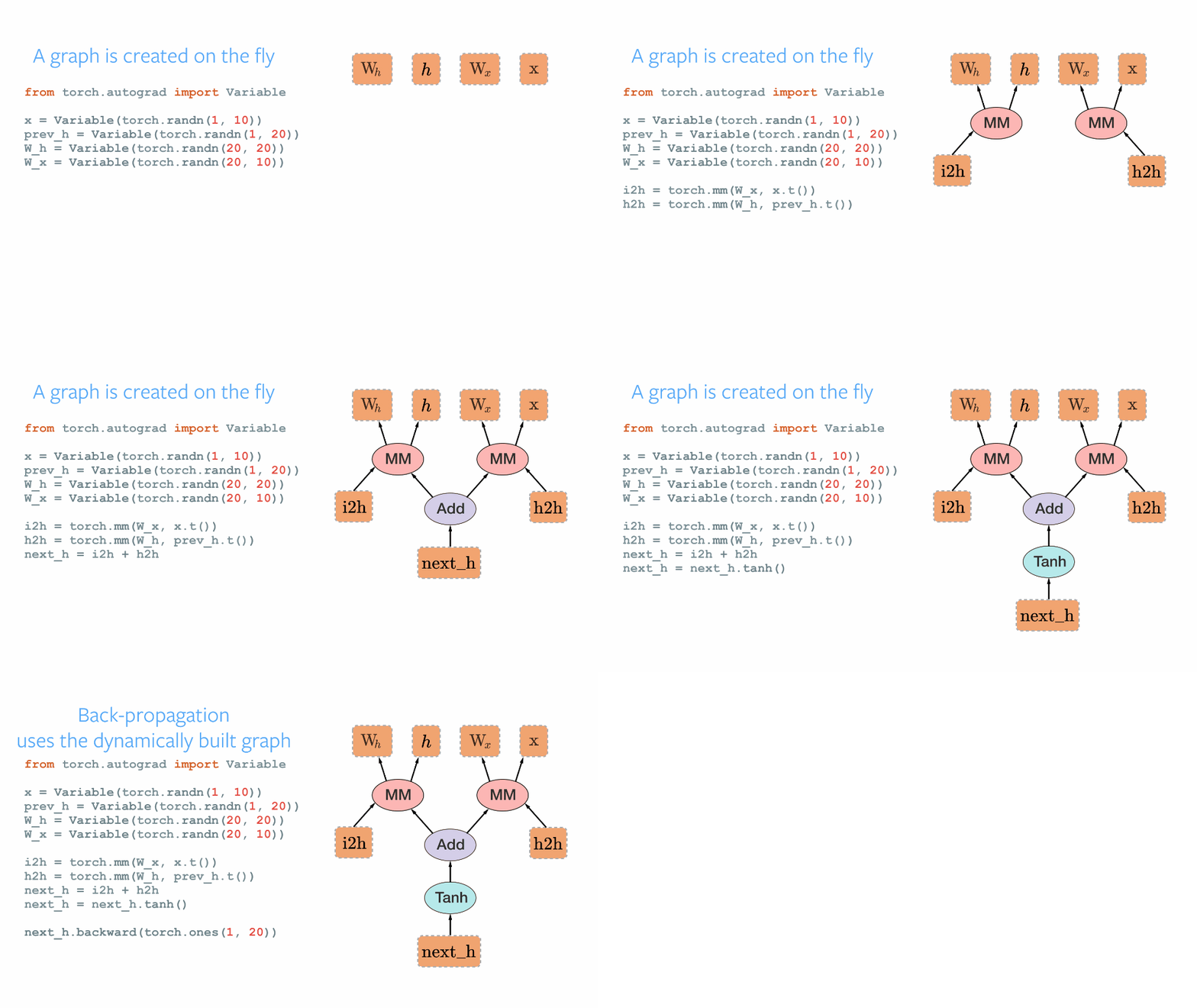 \n*PyTorch dynamic computational graph — source: http://pytorch.org/about/*\n\n###### [Go to top](#top)"},{"metadata":{"_uuid":"fb4dee7a83d3fd5c6528b6acb6deb3ede07917c9"},"cell_type":"markdown","source":"
 \n## 4-4-1 Tensors\n**Tensors** are similar to NumPy’s ndarrays, with the addition being that Tensors can also be used on a GPU to accelerate computing."},{"metadata":{"_uuid":"c9fa542c5e81368bf67ba10968825778888cb9ed","trusted":true,"_kg_hide-input":true},"cell_type":"code","source":"from __future__ import print_function\nimport torch","execution_count":null,"outputs":[]},{"metadata":{"_uuid":"428a61e2f48669f3eda674ed89cadd52983d8f07"},"cell_type":"markdown","source":"Construct a 5x3 matrix, uninitialized:"},{"metadata":{"_uuid":"1367d89d0910e7ebbb474dd1f857f83b4ff4aece","trusted":true,"_kg_hide-input":true},"cell_type":"code","source":"x = torch.empty(5, 3)\nprint(x)","execution_count":null,"outputs":[]},{"metadata":{"_uuid":"984addcd6041b2b34506522bccea8efd3f27bf1e"},"cell_type":"markdown","source":"Construct a randomly initialized matrix:\n\n"},{"metadata":{"_uuid":"4410ff53288dfc7790cc40eb209df552d35487d6","trusted":true,"_kg_hide-input":true},"cell_type":"code","source":"x = torch.rand(5, 3)\nprint(x)","execution_count":null,"outputs":[]},{"metadata":{"_uuid":"e0023c417e35ebeabf4bbcd9a3801fd381de4407"},"cell_type":"markdown","source":"Construct a matrix filled zeros and of dtype long:\n\n###### [Go to top](#top)"},{"metadata":{"_uuid":"827868be4fe401a9651ffc9bf95d37812dacb478","trusted":true,"_kg_hide-input":true},"cell_type":"code","source":"x = torch.zeros(5, 3, dtype=torch.long)\nprint(x)","execution_count":null,"outputs":[]},{"metadata":{"_uuid":"40eaebdbaa6cbf7f36e77891789bc1c05274bfb3"},"cell_type":"markdown","source":"Construct a tensor directly from data:\n\n"},{"metadata":{"_uuid":"21956cadded8ec22cb21b2d02ea99132fd016e6a","trusted":true,"_kg_hide-input":true},"cell_type":"code","source":"x = torch.tensor([5.5, 3])\nprint(x)","execution_count":null,"outputs":[]},{"metadata":{"_uuid":"885dbbc02d2e452f03c059e52303c6157064134d"},"cell_type":"markdown","source":"Or create a tensor based on an existing tensor. These methods will reuse properties of the input tensor, e.g. dtype, unless new values are provided by user.\n\n###### [Go to top](#top)"},{"metadata":{"_uuid":"a649ed5e927a0d723397fc89627bb79ff777e221","trusted":true,"_kg_hide-input":true},"cell_type":"code","source":"x = x.new_ones(5, 3, dtype=torch.double) # new_* methods take in sizes\nprint(x)\n\nx = torch.randn_like(x, dtype=torch.float) # override dtype!\nprint(x) # result has the same size","execution_count":null,"outputs":[]},{"metadata":{"_uuid":"bab1c6447f5062d5a931c5e642b0f409d472fda7"},"cell_type":"markdown","source":"Get its size:"},{"metadata":{"_uuid":"62961e53b2bb3f99762d659902f10ef6a3c97332","trusted":true,"_kg_hide-input":true},"cell_type":"code","source":"print(x.size())","execution_count":null,"outputs":[]},{"metadata":{"_uuid":"0a6e5752f4585ad9ae0e0592c33c56b1675626cb"},"cell_type":"markdown","source":"
\n## 4-4-2 Operations\nThere are multiple syntaxes for operations. In the following example, we will take a look at the addition operation.\n\nAddition: syntax 1.\n\n###### [Go to top](#top)"},{"metadata":{"_uuid":"aeffc489a8e0c446c7c8532054e1892021b1bfcd","trusted":true,"_kg_hide-input":true},"cell_type":"code","source":"y = torch.rand(5, 3)\nprint(x + y)","execution_count":null,"outputs":[]},{"metadata":{"_uuid":"92344324d330a3adbe7ac2c4f612fb55953249b2"},"cell_type":"markdown","source":"Addition: syntax 2\n\n"},{"metadata":{"_uuid":"75b4d2d34207835bd33382894e86416cb7257dbe","trusted":true,"_kg_hide-input":true},"cell_type":"code","source":"print(torch.add(x, y))","execution_count":null,"outputs":[]},{"metadata":{"_uuid":"f062bcc0e8a5d5c927ad8cde707bced9c569054d"},"cell_type":"markdown","source":"Addition: providing an output **tensor** as argument.\n\n"},{"metadata":{"_uuid":"65caf77ef11dde7550d2ee7b19f9acec6d101840","trusted":true,"_kg_hide-input":true},"cell_type":"code","source":"result = torch.empty(5, 3)\ntorch.add(x, y, out=result)\nprint(result)","execution_count":null,"outputs":[]},{"metadata":{"_uuid":"0cb16fa384dea2e2f02cc2169be3f2eed37fa3fd"},"cell_type":"markdown","source":"
\n# 5- Conclusion\nIn this kernel we have just tried to create a **comprehensive deep learning workflow** for helping you to start your jounery in DL.\nsurly it is not **completed yet**!! also I want to hear your voice to improve kernel together."}],"metadata":{"kernelspec":{"display_name":"Python 3","language":"python","name":"python3"},"language_info":{"name":"python","version":"3.6.6","mimetype":"text/x-python","codemirror_mode":{"name":"ipython","version":3},"pygments_lexer":"ipython3","nbconvert_exporter":"python","file_extension":".py"}},"nbformat":4,"nbformat_minor":1}