{"cells":[{"metadata":{"_uuid":"7f6c3fcefecc375f4996f9c41351452c97920dc0"},"cell_type":"markdown","source":"## What is Attention?\n* **Attention** is ***simply a vector, often the outputs of dense layer using softmax function.***\n* Before Attention mechanism, ***translation relies on reading a complete sentence and compress all information into a fixed-length vector***, as you can image, a sentence with hundreds of words represented by several words will surely lead to information loss, inadequate translation, etc.\n\n## Attention Architecture with Idea Behind it.\n\n* The **basic idea:** each time the **model predicts an output word, it only uses parts of an input where the most relevant information is concentrated instead of an entire sentence.** In ***other words, it only pays attention to some input words. Let’s investigate how this is implemented.***\n\n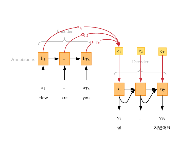![](https://cdn-images-1.medium.com/max/800/1*9Lcq9ni9aujScFYyyHRhhA.png)\n\n* Encoder works as usual, and the**difference is only on the decoder’s part.** As you can see from a picture, ***the decoder’s hidden state is computed with a context vector, the previous output and the previous hidden state. But now we use not a single context vector c, but a separate context vector c_i for each target word.***\n* These context vectors are **computed as a weighted sum of annotations generated by the encoder.** In **Bahdanau’s paper, they use a Bidirectional LSTM, so these annotations are concatenations of hidden states in forward and backward directions.**\n* The weight of each annotation is computed by an alignment model which scores how well the **inputs and the output match.** An alignment model is a **feedforward neural network**, for instance. In general, it can be any other model as well.\n* As a result, the **alphas — the weights of hidden states when computing a context vector — show how important a given annotation is in deciding the next state and generating the output word. These are the attention scores.**\n\n## Why Attention?\n\n* The **core of Probabilistic Language Model** is to **assign a probability to a sentence by Markov Assumption.** Due to the nature of sentences that consist of different numbers of words, RNN is naturally introduced to model the **conditional probability among words.**\n![](https://cdn-images-1.medium.com/max/800/0*SX7ClVkt8w9J39ed.)\n\n**Vanilla RNN (the classic one) often gets trapped when modeling:**\n\n* ***Structure Dilemma:*** in real world, **the length of outputs and inputs can be totally different**, while **Vanilla RNN** can only **handle fixed-length problem which is difficult for the alignment.** Consider an ***EN-FR translation examples: “he doesn’t like apples” → “Il n’aime pas les pommes”.***\n* ***Mathematical Nature:*** it suffers from **Gradient Vanishing/Exploding** which means ***it is hard to train when sentences are long enough (maybe at most 4 words).***\n* ***Translation often requires arbitrary input length and out put length, to deal with the deficits above, encoder-decoder model is adopted and basic RNN cell is changed to GRU or LSTM cell, hyperbolic tangent activation is replaced by ReLU. We use GRU cell here.***\n\n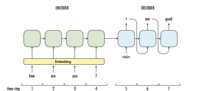![](https://cdn-images-1.medium.com/max/800/0*VwQyyHLPDgEWSD-2.)\n\n* **Embedding layer** maps **discrete words into dense vectors for computational efficiency**. Then **embedded word vectors are fed into encoder**, aka ***GRU cells sequentially.*** What happened during **encoding?** Information flows from left to right and **each word vector** is **learned according to not only current input but also all previous words.** When **the sentence is completely read, encoder generates an output and a hidden state at timestep 4 for further processing.** For ***encoding part, decoder (GRUs as well) grabs the hidden state from encoder, trained by teacher forcing (a mode that previous cell’s output as current input), then generate translation words sequentially.***\n\n* It seems amazing as this model can be applied to **N-to-M sequence**, yet there still is **one main deficit left unsolved: is one hidden state really enough?**\n\n## How does attention work?\n\n![](https://cdn-images-1.medium.com/max/800/0*VrRTrruwf2BtW4t5.)\n\n* Similar to the **basic encoder-decoder architecture,** this fancy mechanism **plug a context vector into the gap between encoder and decoder.** According to the schematic above, **blue represents encoder** and **red represents decoder;** and we could see that **context vector takes all cells’ outputs as input to compute the probability distribution of source language words for each single word decoder wants to generate.** By utilizing this mechanism, **it is possible for decoder to capture somewhat global information rather than solely to infer based on one hidden state.**\n* And to **build context vector is fairly simple.** For a **fixed target word**, ***first***, we **loop over all encoders’ states to compare target** and **source states to generate scores for each state in encoders.** Then we could **use softmax to normalize all scores, which generates the probability distribution conditioned on target states.** At last, the ***weights are introduced to make context vector easy to train. That’s it. Math is shown below:***\n\n![](https://cdn-images-1.medium.com/max/800/0*4y96boGNMiNVHNo8.)\n\n**To understand the seemingly complicated math, we need to keep three key points in mind:**\n* ***During decoding,context vectors are computed for every output word.*** So we will have a **2D matrix whose size is # of target words multiplied by # of source words.** Equation **(1) demonstrates how to compute a single value given one target word and a set of source word.**\n* **Once context vector is computed, attention vector** could be computed by **context vector, target word, and attention function f.**\n* We need **attention mechanism to be trainable**. According to equation **(4), both styles offer the trainable weights (W in Luong’s, W1 and W2 in Bahdanau’s). Thus, different styles may result in different performance.**\n\n## Attention Scoring\n### Inputs to the scoring function\nLet's start by looking at the inputs we'll give to the scoring function. We will assume we're in the first step in the decoging phase. The first input to the scoring function is the hidden state of decoder (assuming a toy RNN with three hidden nodes -- not usable in real life, but easier to illustrate):"},{"metadata":{"trusted":true,"_uuid":"94674cfb193c3f311d3689c02859d99d3fe978a6"},"cell_type":"code","source":"dec_hidden_state = [5,1,20]","execution_count":null,"outputs":[]},{"metadata":{"_uuid":"99ceea530ce3ab9771ae36d3cf6305efe5036321"},"cell_type":"markdown","source":"Let's visualize this vector:"},{"metadata":{"trusted":true,"_uuid":"37561214e9b4dda80487afafca91cc09c810525f"},"cell_type":"code","source":"%matplotlib inline\nimport numpy as np\nimport matplotlib.pyplot as plt\nimport seaborn as sns\n\n# Let's visualize our decoder hidden state\nplt.figure(figsize=(1.5, 4.5))\nsns.heatmap(np.transpose(np.matrix(dec_hidden_state)), annot=True, cmap=sns.light_palette(\"purple\", as_cmap=True), linewidths=1)","execution_count":null,"outputs":[]},{"metadata":{"_uuid":"a8f136f39ed24145145f1cb62215f34d84da4687"},"cell_type":"markdown","source":"Our first scoring function will score a single annotation (encoder hidden state), which looks like this:"},{"metadata":{"trusted":true,"_uuid":"4bf3cbb8dabe711887881ed14d6c3a31aab58e89"},"cell_type":"code","source":"annotation = [3,12,45] #e.g. Encoder hidden state","execution_count":null,"outputs":[]},{"metadata":{"trusted":true,"_uuid":"5dce227099522428a7d2dc101c5773ad1b424ab2"},"cell_type":"code","source":"# Let's visualize the single annotation\nplt.figure(figsize=(1.5, 4.5))\nsns.heatmap(np.transpose(np.matrix(annotation)), annot=True, cmap=sns.light_palette(\"orange\", as_cmap=True), linewidths=1)","execution_count":null,"outputs":[]},{"metadata":{"_uuid":"d70d2be3873409f45565e88db40b8c69405f0217"},"cell_type":"markdown","source":"### IMPLEMENT: Scoring a Single Annotation\nLet's calculate the dot product of a single annotation. Numpy's [dot()](https://docs.scipy.org/doc/numpy/reference/generated/numpy.dot.html) is a good candidate for this operation"},{"metadata":{"trusted":true,"_uuid":"9c502458c6fe9063c5f8bbfdbf39889b1b91b6e8"},"cell_type":"code","source":"def single_dot_attention_score(dec_hidden_state, enc_hidden_state):\n    # TODO: return the dot product of the two vectors\n    return np.dot(dec_hidden_state, enc_hidden_state)\n    \nsingle_dot_attention_score(dec_hidden_state, annotation)","execution_count":null,"outputs":[]},{"metadata":{"_uuid":"f9d8f5b04498e4e052aa15ad926352d8e351367f"},"cell_type":"markdown","source":"\n### Annotations Matrix\nLet's now look at scoring all the annotations at once. To do that, here's our annotation matrix:"},{"metadata":{"trusted":true,"_uuid":"71356443c44bd4e943b35e6c0d603b652e5217ba"},"cell_type":"code","source":"annotations = np.transpose([[3,12,45], [59,2,5], [1,43,5], [4,3,45.3]])","execution_count":null,"outputs":[]},{"metadata":{"_uuid":"d1a291801967f085998926fe9f4c98c7d4eb6047"},"cell_type":"markdown","source":"And it can be visualized like this (each column is a hidden state of an encoder time step):"},{"metadata":{"trusted":true,"_uuid":"d51d0c5f882a94d8f6ae0d87be87a04fb2aa5d3a"},"cell_type":"code","source":"# Let's visualize our annotation (each column is an annotation)\nax = sns.heatmap(annotations, annot=True, cmap=sns.light_palette(\"orange\", as_cmap=True), linewidths=1)","execution_count":null,"outputs":[]},{"metadata":{"_uuid":"0b4f44ea4813f1c80d3042e0745681b17e1d3467"},"cell_type":"markdown","source":"### IMPLEMENT: Scoring All Annotations at Once\nLet's calculate the scores of all the annotations in one step using matrix multiplication. Let's continue to us the dot scoring method\n\n<img src=\"http://yaox023.com/%E6%B7%B1%E5%BA%A6%E5%AD%A6%E4%B9%A0/RNN/attention%E7%90%86%E8%AE%BA/Attention_python%E6%BC%94%E7%A4%BA/images/scoring_functions.png\" />\n\nTo do that, we'll have to transpose `dec_hidden_state` and [matrix multiply](https://docs.scipy.org/doc/numpy/reference/generated/numpy.matmul.html) it with `annotations`."},{"metadata":{"trusted":true,"_uuid":"8a46ae1d2a8b4b209ea48edc3d57d30ceecd2ff7"},"cell_type":"code","source":"def dot_attention_score(dec_hidden_state, annotations):\n    # TODO: return the product of dec_hidden_state transpose and enc_hidden_states\n    return np.matmul(np.transpose(dec_hidden_state), annotations)\n    \nattention_weights_raw = dot_attention_score(dec_hidden_state, annotations)\nattention_weights_raw","execution_count":null,"outputs":[]},{"metadata":{"_uuid":"892c876f4cb0d17da2dc115ff2518852fda95408"},"cell_type":"markdown","source":"Looking at these scores, can you guess which of the four vectors will get the most attention from the decoder at this time step?\n\n## Softmax\nNow that we have our scores, let's apply softmax:\n<img src=\"http://yaox023.com/%E6%B7%B1%E5%BA%A6%E5%AD%A6%E4%B9%A0/RNN/attention%E7%90%86%E8%AE%BA/Attention_python%E6%BC%94%E7%A4%BA/images/softmax.png\" />"},{"metadata":{"trusted":true,"_uuid":"ce5d157db831947caaf360ac003f601a916c1c1d"},"cell_type":"code","source":"def softmax(x):\n    x = np.array(x, dtype=np.float128)\n    e_x = np.exp(x)\n    return e_x / e_x.sum(axis=0) \n\nattention_weights = softmax(attention_weights_raw)\nattention_weights","execution_count":null,"outputs":[]},{"metadata":{"_uuid":"d847c3590c023ef5bd70529ddbe60e1ce0d2e580"},"cell_type":"markdown","source":"Even when knowing which annotation will get the most focus, it's interesting to see how drastic softmax makes the end score become. The first and last annotation had the respective scores of 927 and 929. But after softmax, the attention they'll get is 0.12 and 0.88 respectively.\n\n# Applying the scores back on the annotations\nNow that we have our scores, let's multiply each annotation by its score to proceed closer to the attention context vector. This is the multiplication part of this formula (we'll tackle the summation part in the latter cells)\n\n<img src=\"http://yaox023.com/%E6%B7%B1%E5%BA%A6%E5%AD%A6%E4%B9%A0/RNN/attention%E7%90%86%E8%AE%BA/Attention_python%E6%BC%94%E7%A4%BA/images/Context_vector.png\" />"},{"metadata":{"trusted":true,"_uuid":"291f4b057a14a02adfee3e3ea74940f6ab7dfaec"},"cell_type":"code","source":"def apply_attention_scores(attention_weights, annotations):\n    # TODO: Multiple the annotations by their weights\n    return attention_weights * annotations\n\napplied_attention = apply_attention_scores(attention_weights, annotations)\napplied_attention","execution_count":null,"outputs":[]},{"metadata":{"_uuid":"35576668ac1a7eacbdc62a95620ca7367703125c"},"cell_type":"markdown","source":"Let's visualize how the context vector looks now that we've applied the attention scores back on it:"},{"metadata":{"trusted":true,"_uuid":"7ab7a984f5351c7a721af40717bb5503f31d701a"},"cell_type":"code","source":"# Let's visualize our annotations after applying attention to them\nax = sns.heatmap(applied_attention, annot=True, cmap=sns.light_palette(\"orange\", as_cmap=True), linewidths=1)","execution_count":null,"outputs":[]},{"metadata":{"_uuid":"4a231097683190f2826b7095ad6bfc88b592fcf8"},"cell_type":"markdown","source":"Contrast this with the raw annotations visualized earlier in the notebook, and we can see that the second and third annotations (columns) have been nearly wiped out. The first annotation maintains some of its value, and the fourth annotation is the most pronounced.\n\n# Calculating the Attention Context Vector\nAll that remains to produce our attention context vector now is to sum up the four columns to produce a single attention context vector\n"},{"metadata":{"trusted":true,"_uuid":"d646dcb81626f800119d4b5bda976643125a6adf"},"cell_type":"code","source":"def calculate_attention_vector(applied_attention):\n    return np.sum(applied_attention, axis=1)\n\nattention_vector = calculate_attention_vector(applied_attention)\nattention_vector","execution_count":null,"outputs":[]},{"metadata":{"scrolled":false,"trusted":true,"_uuid":"5f036492764ee5916cdf9745374369770f45c800"},"cell_type":"code","source":"# Let's visualize the attention context vector\nplt.figure(figsize=(1.5, 4.5))\nsns.heatmap(np.transpose(np.matrix(attention_vector)), annot=True, cmap=sns.light_palette(\"Blue\", as_cmap=True), linewidths=1)","execution_count":null,"outputs":[]},{"metadata":{"_uuid":"866be2125e8174fc17bfa92a035d3a4ed375348f"},"cell_type":"markdown","source":"Now that we have the context vector, we can concatinate it with the hidden state and pass it through a hidden layer to produce the the result of this decoding time step.\n\n### References : \n\n[1] Vinyals, Oriol, et al. Show and tell: A neural image caption generator. arXiv:1411.4555 (2014).  \n[2] Bahdanau, Dzmitry, Kyunghyun Cho, and Yoshua Bengio. Neural machine translation by jointly learning to align and translate. arXiv:1409.0473 (2014).  \n[3] Cho, Kyunghyun, Aaron Courville, and Yoshua Bengio. Describing Multimedia Content using Attention-based Encoder–Decoder Networks. arXiv:1507.01053 (2015)  \n[4] Xu, Kelvin, et al. Show, attend and tell: Neural image caption generation with visual attention. arXiv:1502.03044 (2015).  \n[5] Sukhbaatar, Sainbayar, Jason Weston, and Rob Fergus. End-to-end memory networks. Advances in Neural Information Processing Systems. (2015).  \n[6] Joulin, Armand, and Tomas Mikolov. Inferring Algorithmic Patterns with Stack-Augmented Recurrent Nets. arXiv:1503.01007 (2015).  \n[7] Hermann, Karl Moritz, et al. Teaching machines to read and comprehend. Advances in Neural Information Processing Systems. (2015).  \n[8] Raffel, Colin, and Daniel PW Ellis. Feed-Forward Networks with Attention Can Solve Some Long-Term Memory Problems. arXiv:1512.08756 (2015).  \n[9] Vaswani, A., Shazeer, N., Parmar, N., Uszkoreit, J., Jones, L., & Gomez, A. et al. . Attention Is All You Need. arXiv: 1706.03762 (2017).  "}],"metadata":{"anaconda-cloud":{},"kernelspec":{"display_name":"Python 3","language":"python","name":"python3"},"language_info":{"name":"python","version":"3.6.6","mimetype":"text/x-python","codemirror_mode":{"name":"ipython","version":3},"pygments_lexer":"ipython3","nbconvert_exporter":"python","file_extension":".py"}},"nbformat":4,"nbformat_minor":1}