{"cells":[{"metadata":{"_kg_hide-input":true,"execution":{"iopub.execute_input":"2020-10-18T14:05:00.344987Z","iopub.status.busy":"2020-10-18T14:05:00.343816Z","iopub.status.idle":"2020-10-18T14:05:00.348856Z","shell.execute_reply":"2020-10-18T14:05:00.349524Z"},"papermill":{"duration":0.083251,"end_time":"2020-10-18T14:05:00.349725","exception":false,"start_time":"2020-10-18T14:05:00.266474","status":"completed"},"tags":[],"trusted":true},"cell_type":"code","source":"%%HTML\n","execution_count":null,"outputs":[]},{"metadata":{"papermill":{"duration":0.066164,"end_time":"2020-10-18T14:05:00.61703","exception":false,"start_time":"2020-10-18T14:05:00.550866","status":"completed"},"tags":[]},"cell_type":"markdown","source":"# INGV - Volcanic Eruption Prediction
\n\n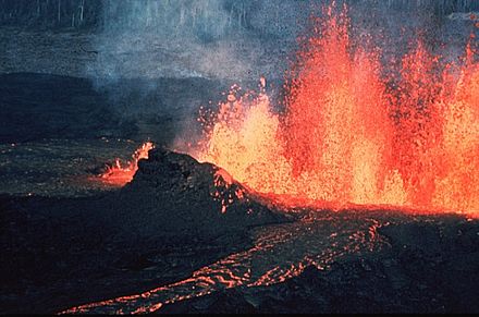\n\n\n## **Content**\n1. [Introduction](#1)\n1. [Libraries and dataset](#2)\n1. [Data overview](#3)\n1. [Visualization](#4)\n - Train data\n - Sensor data\n1. [EDA](#5)\n - Trends between max of each sensor data and time_to_eruption.\n - Trends between minimum of each sensor data and time_to_eruption.\n - Trends between mean of each sensor data and time_to_eruption.\n - Trends between variance of each sensor data and time_to_eruption.\n - Trends 75, 95 and 99 percentiles of each sensor data and time_to_eruption.\n - Trends between count of outlier of each sensor data and time_to_eruption.\n - Sensor down time.\n1. [Application to prediction](#6)"},{"metadata":{"papermill":{"duration":0.066045,"end_time":"2020-10-18T14:05:00.748778","exception":false,"start_time":"2020-10-18T14:05:00.682733","status":"completed"},"tags":[]},"cell_type":"markdown","source":"## **Summary**\n\n1. Checked overview of given data.\n\n1. Checked trends of segments which as large or small(especially smaller than 10 min) time_to_eruption by plots.\n\n1. Visualized relation between descriptive statistics values and time_to_eruption. Especially,\n\n - In small time_to_eruption area (~ 1.0 * 10^7), descriptive statistics value such as variance get larger. \n\n - In large time_to_eruption area (5.0 * 10^7 ~ ), sensor9 has large outlier count at some segment.\n\n - In medium time_to_eruption area (2.0 * 10^7 ~ 4.0 * 10^7), sensor6 tend to have slightly large parcentile(95% and 99%) value.\n \n1. Applied found feature for baseline notebook and confirmed improvement(lb score 6614776 -> 6555212.)."},{"metadata":{"papermill":{"duration":0.067808,"end_time":"2020-10-18T14:05:00.883678","exception":false,"start_time":"2020-10-18T14:05:00.81587","status":"completed"},"tags":[]},"cell_type":"markdown","source":"
\n# Introduction
\n\nDetecting volcanic eruptions before they happen is an important problem that has historically proven to be a very difficult. This is because once an eruption occurs, it can cause extensive damage for many people. \n\nIn this competition, we have to find the way for long-term predictions of the next volcanic eruptions. We need to have an in-depth understanding of the trends of data points, no matter how close or far away from each eruption.\n\nIn this notebook, I'll check given data, and do visualization and eda to get good understanding and insight for the data."},{"metadata":{"papermill":{"duration":0.067917,"end_time":"2020-10-18T14:05:01.018372","exception":false,"start_time":"2020-10-18T14:05:00.950455","status":"completed"},"tags":[]},"cell_type":"markdown","source":"### premise from discussion\n\nI think there are some ambiguity information for given data, but some important points have been made clear in the discussion. Here's a summary of what I've picked up.\n\n- One volcano (https://www.kaggle.com/c/predict-volcanic-eruptions-ingv-oe/discussion/190936)\n\n- Same 10 sensors (https://www.kaggle.com/c/predict-volcanic-eruptions-ingv-oe/discussion/191445)\n\n- unit of time_to_eruption and time span of sensor data records are 0.01s. (https://www.kaggle.com/c/predict-volcanic-eruptions-ingv-oe/discussion/190682)\n\n- Sensor has downtime(https://www.kaggle.com/c/predict-volcanic-eruptions-ingv-oe/discussion/191444)."},{"metadata":{"papermill":{"duration":0.067054,"end_time":"2020-10-18T14:05:01.15165","exception":false,"start_time":"2020-10-18T14:05:01.084596","status":"completed"},"tags":[]},"cell_type":"markdown","source":"
\n# Libraries and dataset
"},{"metadata":{"_cell_guid":"b1076dfc-b9ad-4769-8c92-a6c4dae69d19","_uuid":"8f2839f25d086af736a60e9eeb907d3b93b6e0e5","execution":{"iopub.execute_input":"2020-10-18T14:05:01.298503Z","iopub.status.busy":"2020-10-18T14:05:01.297679Z","iopub.status.idle":"2020-10-18T14:05:02.572697Z","shell.execute_reply":"2020-10-18T14:05:02.571979Z"},"papermill":{"duration":1.354578,"end_time":"2020-10-18T14:05:02.572827","exception":false,"start_time":"2020-10-18T14:05:01.218249","status":"completed"},"tags":[],"trusted":true},"cell_type":"code","source":"import gc\nimport glob\nfrom itertools import chain\n\nimport matplotlib.pyplot as plt\nimport numpy as np\nimport pandas as pd\nfrom plotly.subplots import make_subplots\nimport plotly.graph_objects as go\nfrom tqdm import tqdm\nimport seaborn as sns","execution_count":null,"outputs":[]},{"metadata":{"papermill":{"duration":0.065609,"end_time":"2020-10-18T14:05:02.704853","exception":false,"start_time":"2020-10-18T14:05:02.639244","status":"completed"},"tags":[]},"cell_type":"markdown","source":"There are three kind of files.\n\n- train.csv: trainig data witch includes segment_id and time_to_eruption.\n\n- sample_submission.csv: sample submission file witch includes segment_id and time_to_eruption all 0.\n\n- [train|test]/*.csv: File which contains ten minutes of logs from ten different sensors arrayed around a volcano.\n\nWe have to predict \"time_to_eruption\" of sample_submission."},{"metadata":{"execution":{"iopub.execute_input":"2020-10-18T14:05:02.8444Z","iopub.status.busy":"2020-10-18T14:05:02.843478Z","iopub.status.idle":"2020-10-18T14:05:03.608762Z","shell.execute_reply":"2020-10-18T14:05:03.608052Z"},"papermill":{"duration":0.838424,"end_time":"2020-10-18T14:05:03.608893","exception":false,"start_time":"2020-10-18T14:05:02.770469","status":"completed"},"tags":[],"trusted":true},"cell_type":"code","source":"!ls ../input/predict-volcanic-eruptions-ingv-oe/","execution_count":null,"outputs":[]},{"metadata":{"papermill":{"duration":0.067946,"end_time":"2020-10-18T14:05:03.743685","exception":false,"start_time":"2020-10-18T14:05:03.675739","status":"completed"},"tags":[]},"cell_type":"markdown","source":"Let's load train data and sample_submission."},{"metadata":{"execution":{"iopub.execute_input":"2020-10-18T14:05:03.903229Z","iopub.status.busy":"2020-10-18T14:05:03.902239Z","iopub.status.idle":"2020-10-18T14:05:03.927574Z","shell.execute_reply":"2020-10-18T14:05:03.928673Z"},"papermill":{"duration":0.118406,"end_time":"2020-10-18T14:05:03.928963","exception":false,"start_time":"2020-10-18T14:05:03.810557","status":"completed"},"tags":[],"trusted":true},"cell_type":"code","source":"train = pd.read_csv(\"../input/predict-volcanic-eruptions-ingv-oe/train.csv\")\nsample_submission = pd.read_csv(\"../input/predict-volcanic-eruptions-ingv-oe/sample_submission.csv\")","execution_count":null,"outputs":[]},{"metadata":{"papermill":{"duration":0.072953,"end_time":"2020-10-18T14:05:04.088223","exception":false,"start_time":"2020-10-18T14:05:04.01527","status":"completed"},"tags":[]},"cell_type":"markdown","source":"Second, check what sensor data is available. Sensor data named by \"segment_id\" + \".csv\".\n\nThere are no data which taken in same segment."},{"metadata":{"_kg_hide-output":true,"execution":{"iopub.execute_input":"2020-10-18T14:05:04.230517Z","iopub.status.busy":"2020-10-18T14:05:04.229744Z","iopub.status.idle":"2020-10-18T14:05:04.992185Z","shell.execute_reply":"2020-10-18T14:05:04.991209Z"},"papermill":{"duration":0.837464,"end_time":"2020-10-18T14:05:04.992333","exception":false,"start_time":"2020-10-18T14:05:04.154869","status":"completed"},"tags":[],"trusted":true},"cell_type":"code","source":"segment_csvs = glob.glob(\"../input/predict-volcanic-eruptions-ingv-oe/train/*\")\nsegment_csvs_test = glob.glob(\"../input/predict-volcanic-eruptions-ingv-oe/test/*\")","execution_count":null,"outputs":[]},{"metadata":{"execution":{"iopub.execute_input":"2020-10-18T14:05:05.134464Z","iopub.status.busy":"2020-10-18T14:05:05.133585Z","iopub.status.idle":"2020-10-18T14:05:05.138665Z","shell.execute_reply":"2020-10-18T14:05:05.137896Z"},"papermill":{"duration":0.078062,"end_time":"2020-10-18T14:05:05.138789","exception":false,"start_time":"2020-10-18T14:05:05.060727","status":"completed"},"tags":[],"trusted":true},"cell_type":"code","source":"segment_csvs[0:10]","execution_count":null,"outputs":[]},{"metadata":{"execution":{"iopub.execute_input":"2020-10-18T14:05:05.297544Z","iopub.status.busy":"2020-10-18T14:05:05.292381Z","iopub.status.idle":"2020-10-18T14:05:16.194743Z","shell.execute_reply":"2020-10-18T14:05:16.194053Z"},"papermill":{"duration":10.988372,"end_time":"2020-10-18T14:05:16.19487","exception":false,"start_time":"2020-10-18T14:05:05.206498","status":"completed"},"tags":[],"trusted":true},"cell_type":"code","source":"print(\"Number of files under train/ is:\", len(segment_csvs))\nprint(\"Number of files under test/ is:\", len(segment_csvs_test))\n\nduplicated_segment_id = [segment_id for segment_id in [ test_segment_id.split(\"/\")[-1] for test_segment_id in segment_csvs_test]\n if (segment_id in [ train_segment_id.split(\"/\")[-1] for train_segment_id in segment_csvs])]\n\nprint(\"Segment ids both in train and test are:\", duplicated_segment_id)","execution_count":null,"outputs":[]},{"metadata":{"papermill":{"duration":0.067455,"end_time":"2020-10-18T14:05:16.330279","exception":false,"start_time":"2020-10-18T14:05:16.262824","status":"completed"},"tags":[]},"cell_type":"markdown","source":"There are a lot of sensor data, I'll load following 2 data for explanation."},{"metadata":{"execution":{"iopub.execute_input":"2020-10-18T14:05:16.477411Z","iopub.status.busy":"2020-10-18T14:05:16.476527Z","iopub.status.idle":"2020-10-18T14:05:16.734468Z","shell.execute_reply":"2020-10-18T14:05:16.733574Z"},"papermill":{"duration":0.336199,"end_time":"2020-10-18T14:05:16.734609","exception":false,"start_time":"2020-10-18T14:05:16.39841","status":"completed"},"tags":[],"trusted":true},"cell_type":"code","source":"train_379022420 = pd.read_csv(\"../input/predict-volcanic-eruptions-ingv-oe/train/379022420.csv\")\ntrain_1002275321 = pd.read_csv(\"../input/predict-volcanic-eruptions-ingv-oe/train/1002275321.csv\")","execution_count":null,"outputs":[]},{"metadata":{"papermill":{"duration":0.068427,"end_time":"2020-10-18T14:05:16.871145","exception":false,"start_time":"2020-10-18T14:05:16.802718","status":"completed"},"tags":[]},"cell_type":"markdown","source":"
\n# Data overview
\n\nLet's check overview, data type, NaN of loaded data.\n\ntrain.csv includes segment_id and time_to_eruption. There are 4431 data. \"time_to_eruption\" represents time until the next eruption. This value is target of this competition. \"segment_id\" is ID code for the data segment. Matches the name of the associated data file in [train|test]/*."},{"metadata":{"execution":{"iopub.execute_input":"2020-10-18T14:05:17.029896Z","iopub.status.busy":"2020-10-18T14:05:17.0291Z","iopub.status.idle":"2020-10-18T14:05:17.038092Z","shell.execute_reply":"2020-10-18T14:05:17.037412Z"},"papermill":{"duration":0.098407,"end_time":"2020-10-18T14:05:17.038227","exception":false,"start_time":"2020-10-18T14:05:16.93982","status":"completed"},"tags":[],"trusted":true},"cell_type":"code","source":"train.head()","execution_count":null,"outputs":[]},{"metadata":{"execution":{"iopub.execute_input":"2020-10-18T14:05:17.191969Z","iopub.status.busy":"2020-10-18T14:05:17.19101Z","iopub.status.idle":"2020-10-18T14:05:17.194542Z","shell.execute_reply":"2020-10-18T14:05:17.195437Z"},"papermill":{"duration":0.088673,"end_time":"2020-10-18T14:05:17.195658","exception":false,"start_time":"2020-10-18T14:05:17.106985","status":"completed"},"tags":[],"trusted":true},"cell_type":"code","source":"train.info()","execution_count":null,"outputs":[]},{"metadata":{"papermill":{"duration":0.069422,"end_time":"2020-10-18T14:05:17.335072","exception":false,"start_time":"2020-10-18T14:05:17.26565","status":"completed"},"tags":[]},"cell_type":"markdown","source":"Sample submission includes segment_id and time_to_eruption all 0. As you can see from the number of data under the test seen above, there are 4520 rows."},{"metadata":{"execution":{"iopub.execute_input":"2020-10-18T14:05:17.485603Z","iopub.status.busy":"2020-10-18T14:05:17.484402Z","iopub.status.idle":"2020-10-18T14:05:17.489249Z","shell.execute_reply":"2020-10-18T14:05:17.488568Z"},"papermill":{"duration":0.083779,"end_time":"2020-10-18T14:05:17.489384","exception":false,"start_time":"2020-10-18T14:05:17.405605","status":"completed"},"tags":[],"trusted":true},"cell_type":"code","source":"sample_submission.head()","execution_count":null,"outputs":[]},{"metadata":{"execution":{"iopub.execute_input":"2020-10-18T14:05:17.643565Z","iopub.status.busy":"2020-10-18T14:05:17.642399Z","iopub.status.idle":"2020-10-18T14:05:17.646301Z","shell.execute_reply":"2020-10-18T14:05:17.646894Z"},"papermill":{"duration":0.086737,"end_time":"2020-10-18T14:05:17.647103","exception":false,"start_time":"2020-10-18T14:05:17.560366","status":"completed"},"tags":[],"trusted":true},"cell_type":"code","source":"sample_submission.info()","execution_count":null,"outputs":[]},{"metadata":{"papermill":{"duration":0.070843,"end_time":"2020-10-18T14:05:17.789017","exception":false,"start_time":"2020-10-18T14:05:17.718174","status":"completed"},"tags":[]},"cell_type":"markdown","source":"Next, sensor data. Each file contains ten minutes of logs from ten different sensors arrayed around a volcano. The readings have been normalized within each segment, in part to ensure that the readings fall within the range of int16 values.\n\nFor example, 379022420.csv has float type data and no lack."},{"metadata":{"execution":{"iopub.execute_input":"2020-10-18T14:05:17.95215Z","iopub.status.busy":"2020-10-18T14:05:17.951159Z","iopub.status.idle":"2020-10-18T14:05:17.956718Z","shell.execute_reply":"2020-10-18T14:05:17.955915Z"},"papermill":{"duration":0.095178,"end_time":"2020-10-18T14:05:17.956856","exception":false,"start_time":"2020-10-18T14:05:17.861678","status":"completed"},"tags":[],"trusted":true},"cell_type":"code","source":"train_379022420.head()","execution_count":null,"outputs":[]},{"metadata":{"execution":{"iopub.execute_input":"2020-10-18T14:05:18.108195Z","iopub.status.busy":"2020-10-18T14:05:18.107379Z","iopub.status.idle":"2020-10-18T14:05:18.120799Z","shell.execute_reply":"2020-10-18T14:05:18.119772Z"},"papermill":{"duration":0.090765,"end_time":"2020-10-18T14:05:18.121027","exception":false,"start_time":"2020-10-18T14:05:18.030262","status":"completed"},"tags":[],"trusted":true},"cell_type":"code","source":"train_379022420.info()","execution_count":null,"outputs":[]},{"metadata":{"papermill":{"duration":0.071615,"end_time":"2020-10-18T14:05:18.265714","exception":false,"start_time":"2020-10-18T14:05:18.194099","status":"completed"},"tags":[]},"cell_type":"markdown","source":"But, some sensor data has lack. See following data of 1002275321 segment."},{"metadata":{"execution":{"iopub.execute_input":"2020-10-18T14:05:18.427986Z","iopub.status.busy":"2020-10-18T14:05:18.42715Z","iopub.status.idle":"2020-10-18T14:05:18.432289Z","shell.execute_reply":"2020-10-18T14:05:18.432854Z"},"papermill":{"duration":0.094873,"end_time":"2020-10-18T14:05:18.43304","exception":false,"start_time":"2020-10-18T14:05:18.338167","status":"completed"},"tags":[],"trusted":true},"cell_type":"code","source":"train_1002275321.head()","execution_count":null,"outputs":[]},{"metadata":{"execution":{"iopub.execute_input":"2020-10-18T14:05:18.586748Z","iopub.status.busy":"2020-10-18T14:05:18.585888Z","iopub.status.idle":"2020-10-18T14:05:18.598693Z","shell.execute_reply":"2020-10-18T14:05:18.597711Z"},"papermill":{"duration":0.092432,"end_time":"2020-10-18T14:05:18.598883","exception":false,"start_time":"2020-10-18T14:05:18.506451","status":"completed"},"tags":[],"trusted":true},"cell_type":"code","source":"train_1002275321.info()","execution_count":null,"outputs":[]},{"metadata":{"papermill":{"duration":0.073708,"end_time":"2020-10-18T14:05:18.747291","exception":false,"start_time":"2020-10-18T14:05:18.673583","status":"completed"},"tags":[]},"cell_type":"markdown","source":"
\n# Visualization
\n\nHere, I'll check and visualize train and sensor data, and get a better understanding of these data."},{"metadata":{"papermill":{"duration":0.073975,"end_time":"2020-10-18T14:05:18.895801","exception":false,"start_time":"2020-10-18T14:05:18.821826","status":"completed"},"tags":[]},"cell_type":"markdown","source":"## Train data"},{"metadata":{"trusted":true},"cell_type":"code","source":"g = sns.distplot(train[\"time_to_eruption\"], kde=False, rug=False, color=\"r\")\ng.set_title(\"distribution of time_to_eruption of train data\")","execution_count":null,"outputs":[]},{"metadata":{"papermill":{"duration":0.074744,"end_time":"2020-10-18T14:05:19.477985","exception":false,"start_time":"2020-10-18T14:05:19.403241","status":"completed"},"tags":[]},"cell_type":"markdown","source":"The value of time_to_eruption seems to be about the same number of times. The number decrease at 4e7 and above."},{"metadata":{"papermill":{"duration":0.074653,"end_time":"2020-10-18T14:05:19.628032","exception":false,"start_time":"2020-10-18T14:05:19.553379","status":"completed"},"tags":[]},"cell_type":"markdown","source":"## Sensor data\n\nTo simple visualize, first, I check segment id 379022420 data. For line plots and other plots that cannot be written for 10 sensors at a time, I made the function myself. Some of the dataframes are re-read, but I just prioritized ease of processing, so don't worry about it."},{"metadata":{"papermill":{"duration":0.075868,"end_time":"2020-10-18T14:05:19.829105","exception":false,"start_time":"2020-10-18T14:05:19.753237","status":"completed"},"tags":[]},"cell_type":"markdown","source":"### Line plot of each sensor data."},{"metadata":{"execution":{"iopub.execute_input":"2020-10-18T14:05:19.991109Z","iopub.status.busy":"2020-10-18T14:05:19.989443Z","iopub.status.idle":"2020-10-18T14:05:19.994831Z","shell.execute_reply":"2020-10-18T14:05:19.994071Z"},"papermill":{"duration":0.090415,"end_time":"2020-10-18T14:05:19.994974","exception":false,"start_time":"2020-10-18T14:05:19.904559","status":"completed"},"tags":[],"trusted":true},"cell_type":"code","source":"def crete_lineplot(segment_id):\n df = pd.read_csv(f\"../input/predict-volcanic-eruptions-ingv-oe/train/{segment_id}.csv\") \n graphs = []\n\n for i in range(0, 9 , 5):\n idxs = list(np.array([0, 1, 2, 3, 4]) + i)\n\n fig, axs = plt.subplots(1, 5, sharey=True)\n for k, item in enumerate(idxs):\n g = sns.lineplot(data=df[f\"sensor_{item+1}\"], ax=axs[k], color=\"g\")\n g.set_title(f\"sensor: {item+1}\")\n g.set(ylim=(-10000, 10000))\n graphs.append(g)","execution_count":null,"outputs":[]},{"metadata":{"execution":{"iopub.execute_input":"2020-10-18T14:05:20.158494Z","iopub.status.busy":"2020-10-18T14:05:20.157572Z","iopub.status.idle":"2020-10-18T14:06:07.458315Z","shell.execute_reply":"2020-10-18T14:06:07.45887Z"},"papermill":{"duration":47.386611,"end_time":"2020-10-18T14:06:07.459065","exception":false,"start_time":"2020-10-18T14:05:20.072454","status":"completed"},"tags":[],"trusted":true},"cell_type":"code","source":"crete_lineplot(379022420)","execution_count":null,"outputs":[]},{"metadata":{"papermill":{"duration":0.077549,"end_time":"2020-10-18T14:06:07.615606","exception":false,"start_time":"2020-10-18T14:06:07.538057","status":"completed"},"tags":[]},"cell_type":"markdown","source":"We can see that the value of the second sensor in particular fluctuates greatly.\n\nOther graphs are seems to be quiet."},{"metadata":{"papermill":{"duration":0.077851,"end_time":"2020-10-18T14:06:07.774064","exception":false,"start_time":"2020-10-18T14:06:07.696213","status":"completed"},"tags":[]},"cell_type":"markdown","source":"### Boxplot of each sensor data.\n\nI think detecting outliers will be important, so I'll also write a box-beard diagram."},{"metadata":{"execution":{"iopub.execute_input":"2020-10-18T14:06:10.245723Z","iopub.status.busy":"2020-10-18T14:06:10.244843Z","iopub.status.idle":"2020-10-18T14:06:10.68298Z","shell.execute_reply":"2020-10-18T14:06:10.682297Z"},"papermill":{"duration":2.829752,"end_time":"2020-10-18T14:06:10.683113","exception":false,"start_time":"2020-10-18T14:06:07.853361","status":"completed"},"tags":[],"trusted":true},"cell_type":"code","source":"fig = plt.figure(figsize=(10, 5))\ndf_379022420 = pd.read_csv(f\"../input/predict-volcanic-eruptions-ingv-oe/train/379022420.csv\") \nboxplot = df_379022420.boxplot(column=[f'sensor_{i}' for i in range(1,11)])","execution_count":null,"outputs":[]},{"metadata":{},"cell_type":"markdown","source":"### Violinplot of each sensor data.\n\nI also create violinplot. For plot, I create function we can let data tidy."},{"metadata":{"trusted":true},"cell_type":"code","source":"def tidying_df(df):\n df_tidying = pd.DataFrame(columns=[\"value\", \"sensor\"])\n\n for i in range(1, (df_379022420.shape[1]+1) ):\n df_sensor = df_379022420[[f\"sensor_{i}\"]].copy()\n df_sensor.columns = [\"value\"]\n df_sensor[\"sensor\"] = f\"sensor_{i}\"\n \n df_tidying = pd.concat([df_tidying, df_sensor], axis=0, ignore_index=True)\n\n return df_tidying","execution_count":null,"outputs":[]},{"metadata":{"trusted":true},"cell_type":"code","source":"df_379022420_tidy = tidying_df(df_379022420)","execution_count":null,"outputs":[]},{"metadata":{"trusted":true},"cell_type":"code","source":"df_379022420_tidy.head()","execution_count":null,"outputs":[]},{"metadata":{"trusted":true},"cell_type":"code","source":"fig = plt.figure(figsize=(10, 5))\nsns.violinplot(data=df_379022420_tidy, x=\"sensor\" , y=\"value\")","execution_count":null,"outputs":[]},{"metadata":{"papermill":{"duration":0.082712,"end_time":"2020-10-18T14:06:11.325077","exception":false,"start_time":"2020-10-18T14:06:11.242365","status":"completed"},"tags":[]},"cell_type":"markdown","source":"### Distplot of each sensor data.\n\nI'll plot distplot of each sensor data. First, I create crete_distplot in convenience."},{"metadata":{"execution":{"iopub.execute_input":"2020-10-18T14:06:11.496444Z","iopub.status.busy":"2020-10-18T14:06:11.495628Z","iopub.status.idle":"2020-10-18T14:06:11.50026Z","shell.execute_reply":"2020-10-18T14:06:11.500974Z"},"papermill":{"duration":0.095686,"end_time":"2020-10-18T14:06:11.50115","exception":false,"start_time":"2020-10-18T14:06:11.405464","status":"completed"},"tags":[],"trusted":true},"cell_type":"code","source":"train[train[\"segment_id\"] == 379022420]","execution_count":null,"outputs":[]},{"metadata":{"execution":{"iopub.execute_input":"2020-10-18T14:06:11.675401Z","iopub.status.busy":"2020-10-18T14:06:11.674389Z","iopub.status.idle":"2020-10-18T14:06:11.677808Z","shell.execute_reply":"2020-10-18T14:06:11.677069Z"},"papermill":{"duration":0.095377,"end_time":"2020-10-18T14:06:11.677952","exception":false,"start_time":"2020-10-18T14:06:11.582575","status":"completed"},"tags":[],"trusted":true},"cell_type":"code","source":"def crete_distplot(segment_id):\n df = pd.read_csv(f\"../input/predict-volcanic-eruptions-ingv-oe/train/{segment_id}.csv\") \n graphs = []\n\n for i in range(0, 9 , 5):\n idxs = list(np.array([0, 1, 2, 3, 4]) + i)\n\n fig, axs = plt.subplots(1, 5, sharey=True)\n for k, item in enumerate(idxs):\n g = sns.distplot(df[f\"sensor_{item+1}\"], ax=axs[k], color=\"y\")\n g.set_title(f\"sensor: {item+1}\")\n g.set(ylim=(0, 0.0025))\n graphs.append(g)","execution_count":null,"outputs":[]},{"metadata":{"papermill":{"duration":0.080425,"end_time":"2020-10-18T14:06:11.839178","exception":false,"start_time":"2020-10-18T14:06:11.758753","status":"completed"},"tags":[]},"cell_type":"markdown","source":"The plots seems to be a left-right target. The average seems to be zero. Variance seems to be different by sensors."},{"metadata":{"execution":{"iopub.execute_input":"2020-10-18T14:06:12.154906Z","iopub.status.busy":"2020-10-18T14:06:12.154126Z","iopub.status.idle":"2020-10-18T14:06:14.834698Z","shell.execute_reply":"2020-10-18T14:06:14.833959Z"},"papermill":{"duration":2.9137,"end_time":"2020-10-18T14:06:14.834821","exception":false,"start_time":"2020-10-18T14:06:11.921121","status":"completed"},"tags":[],"trusted":true},"cell_type":"code","source":"crete_distplot(379022420)","execution_count":null,"outputs":[]},{"metadata":{"papermill":{"duration":0.083388,"end_time":"2020-10-18T14:06:15.002023","exception":false,"start_time":"2020-10-18T14:06:14.918635","status":"completed"},"tags":[]},"cell_type":"markdown","source":"### pair plot of each sensor data.\n\nNext, I plot pair plot. There doesn't seem to be any similarities in trends between the sensor data."},{"metadata":{"execution":{"iopub.execute_input":"2020-10-18T14:06:15.175727Z","iopub.status.busy":"2020-10-18T14:06:15.174888Z","iopub.status.idle":"2020-10-18T14:06:59.894746Z","shell.execute_reply":"2020-10-18T14:06:59.669835Z"},"papermill":{"duration":44.808726,"end_time":"2020-10-18T14:06:59.894991","exception":false,"start_time":"2020-10-18T14:06:15.086265","status":"completed"},"tags":[],"trusted":true},"cell_type":"code","source":"sns.pairplot(df_379022420)","execution_count":null,"outputs":[]},{"metadata":{"papermill":{"duration":0.166,"end_time":"2020-10-18T14:07:00.22884","exception":false,"start_time":"2020-10-18T14:07:00.06284","status":"completed"},"tags":[]},"cell_type":"markdown","source":"### question\n\nData which time_to_eruption is smaller than 60000 represents eruption in it's value and graph?"},{"metadata":{"execution":{"iopub.execute_input":"2020-10-18T14:07:00.576683Z","iopub.status.busy":"2020-10-18T14:07:00.575551Z","iopub.status.idle":"2020-10-18T14:07:00.580711Z","shell.execute_reply":"2020-10-18T14:07:00.579973Z"},"papermill":{"duration":0.186809,"end_time":"2020-10-18T14:07:00.580841","exception":false,"start_time":"2020-10-18T14:07:00.394032","status":"completed"},"tags":[],"trusted":true},"cell_type":"code","source":"train[train[\"time_to_eruption\"] < 60000]","execution_count":null,"outputs":[]},{"metadata":{"papermill":{"duration":0.166673,"end_time":"2020-10-18T14:07:00.919081","exception":false,"start_time":"2020-10-18T14:07:00.752408","status":"completed"},"tags":[]},"cell_type":"markdown","source":"I create new function which can plot lineplot with supplementary wire. "},{"metadata":{"execution":{"iopub.execute_input":"2020-10-18T14:07:01.271115Z","iopub.status.busy":"2020-10-18T14:07:01.269928Z","iopub.status.idle":"2020-10-18T14:07:01.273833Z","shell.execute_reply":"2020-10-18T14:07:01.27462Z"},"papermill":{"duration":0.185831,"end_time":"2020-10-18T14:07:01.274841","exception":false,"start_time":"2020-10-18T14:07:01.08901","status":"completed"},"tags":[],"trusted":true},"cell_type":"code","source":"def crete_lineplot_with_supplementarywire(segment_id, xs):\n df = pd.read_csv(f\"../input/predict-volcanic-eruptions-ingv-oe/train/{segment_id}.csv\") \n graphs = []\n\n for i in range(0, 9 , 5):\n idxs = list(np.array([0, 1, 2, 3, 4]) + i)\n\n fig, axs = plt.subplots(1, 5, sharey=True)\n for k, item in enumerate(idxs):\n g = sns.lineplot(data=df[f\"sensor_{item+1}\"], ax=axs[k])\n \n for supplementarywire_x in xs:\n axs[k].plot([supplementarywire_x, supplementarywire_x], [-10000, 10000], c='r', ls='--')\n g.set_title(f\"sensor: {item+1}\")\n g.set(ylim=(-10000, 10000))\n graphs.append(g)","execution_count":null,"outputs":[]},{"metadata":{"execution":{"iopub.execute_input":"2020-10-18T14:07:01.616801Z","iopub.status.busy":"2020-10-18T14:07:01.615879Z","iopub.status.idle":"2020-10-18T14:07:49.027904Z","shell.execute_reply":"2020-10-18T14:07:49.027086Z"},"papermill":{"duration":47.586954,"end_time":"2020-10-18T14:07:49.028055","exception":false,"start_time":"2020-10-18T14:07:01.441101","status":"completed"},"tags":[],"trusted":true},"cell_type":"code","source":"crete_lineplot_with_supplementarywire(1658693785, [1300, 27000])","execution_count":null,"outputs":[]},{"metadata":{"papermill":{"duration":0.165154,"end_time":"2020-10-18T14:07:49.361719","exception":false,"start_time":"2020-10-18T14:07:49.196565","status":"completed"},"tags":[]},"cell_type":"markdown","source":"Huuum.... It doesn't look so bad when we say there are signals at 250 second intervals..."},{"metadata":{"execution":{"iopub.execute_input":"2020-10-18T14:07:49.717572Z","iopub.status.busy":"2020-10-18T14:07:49.716729Z","iopub.status.idle":"2020-10-18T14:08:37.248448Z","shell.execute_reply":"2020-10-18T14:08:37.247764Z"},"papermill":{"duration":47.71836,"end_time":"2020-10-18T14:08:37.24858","exception":false,"start_time":"2020-10-18T14:07:49.53022","status":"completed"},"tags":[],"trusted":true},"cell_type":"code","source":"crete_lineplot_with_supplementarywire(1626437563, [13000, 53000])","execution_count":null,"outputs":[]},{"metadata":{"papermill":{"duration":0.168814,"end_time":"2020-10-18T14:08:37.588103","exception":false,"start_time":"2020-10-18T14:08:37.419289","status":"completed"},"tags":[]},"cell_type":"markdown","source":"The supplementary line on sensor2 looks like good..."},{"metadata":{"papermill":{"duration":0.170478,"end_time":"2020-10-18T14:08:37.928839","exception":false,"start_time":"2020-10-18T14:08:37.758361","status":"completed"},"tags":[]},"cell_type":"markdown","source":"
\n# EDA
"},{"metadata":{"papermill":{"duration":0.170731,"end_time":"2020-10-18T14:08:38.270163","exception":false,"start_time":"2020-10-18T14:08:38.099432","status":"completed"},"tags":[]},"cell_type":"markdown","source":"Here, let's search trends for good represents time until the next eruption."},{"metadata":{"papermill":{"duration":0.170633,"end_time":"2020-10-18T14:08:38.611096","exception":false,"start_time":"2020-10-18T14:08:38.440463","status":"completed"},"tags":[]},"cell_type":"markdown","source":"## Relation between time_to_eruption and descriptive statistics value\n\nI tried to plot relation between time_to_eruption and following descriptive statistics values.\n\n- max\n\n- minimum\n\n- mean\n\n- variance\n\n- 75, 95 and 99 percentiles\n\n- count of outliners\n\nThis is because, we can guess that there might be some signs in 10 minutes sensor datas before eruption. If we found that in descriptive statistics value of sensor datas, we can use them for good prediction."},{"metadata":{"papermill":{"duration":0.170907,"end_time":"2020-10-18T14:08:38.952726","exception":false,"start_time":"2020-10-18T14:08:38.781819","status":"completed"},"tags":[]},"cell_type":"markdown","source":"### Preparation.\n\nI'll calculate above values for each train data."},{"metadata":{"execution":{"iopub.execute_input":"2020-10-18T14:08:39.307089Z","iopub.status.busy":"2020-10-18T14:08:39.306102Z","iopub.status.idle":"2020-10-18T14:08:39.309339Z","shell.execute_reply":"2020-10-18T14:08:39.308718Z"},"papermill":{"duration":0.184816,"end_time":"2020-10-18T14:08:39.309475","exception":false,"start_time":"2020-10-18T14:08:39.124659","status":"completed"},"tags":[],"trusted":true},"cell_type":"code","source":"def count_outlier(df, j):\n q1 = np.percentile(df[f\"sensor_{j}\"], 25, axis=0)\n q3 = np.percentile(df[f\"sensor_{j}\"], 75, axis=0)\n \n max = 2.5*q3 - 1.5*q1\n min = -0.5*q3 - 1.5*q1\n \n return (len(df[f\"sensor_{j}\"][df[f\"sensor_{j}\"] > max] + len(df[f\"sensor_{j}\"][df[f\"sensor_{j}\"] < min])))","execution_count":null,"outputs":[]},{"metadata":{"trusted":true},"cell_type":"code","source":"!ls ../input/ingv-sensor-processed","execution_count":null,"outputs":[]},{"metadata":{"execution":{"iopub.execute_input":"2020-10-18T14:08:39.695569Z","iopub.status.busy":"2020-10-18T14:08:39.694688Z","iopub.status.idle":"2020-10-18T14:08:39.869743Z","shell.execute_reply":"2020-10-18T14:08:39.868992Z"},"papermill":{"duration":0.385235,"end_time":"2020-10-18T14:08:39.869868","exception":false,"start_time":"2020-10-18T14:08:39.484633","status":"completed"},"tags":[],"trusted":true},"cell_type":"code","source":"#for i, segment_id in tqdm(enumerate(train[\"segment_id\"])):\n# df_segment_id = pd.read_csv(f\"../input/predict-volcanic-eruptions-ingv-oe/train/{segment_id}.csv\").fillna(0)\n# \n# for j in range(10):\n# train.loc[i, f\"sensor_{j+1}_max\"] = np.max(df_segment_id.fillna(0), axis=0)[j]\n# train.loc[i, f\"sensor_{j+1}_min\"] = np.min(df_segment_id.fillna(0), axis=0)[j]\n# train.loc[i, f\"sensor_{j+1}_mean\"] = np.mean(df_segment_id.fillna(0), axis=0)[j]\n# train.loc[i, f\"sensor_{j+1}_var\"] = np.var(df_segment_id.fillna(0), axis=0)[j]\n# train.loc[i, f\"sensor_{j+1}_75_percentile\"] = np.percentile(df_segment_id, 75, axis=0)[j]\n# train.loc[i, f\"sensor_{j+1}_95_percentile\"] = np.percentile(df_segment_id, 95, axis=0)[j]\n# train.loc[i, f\"sensor_{j+1}_99_percentile\"] = np.percentile(df_segment_id, 99, axis=0)[j]\n# train.loc[i, f\"sensor_{j+1}_outlier\"] = count_outlier(df_segment_id, j+1)\n# train.loc[i, f\"sensor_{j+1}_null\"] = 1 if df_segment_id.isnull().any()[j] else 0\n\n#To save memory, I use processed data in my other notebook. \n#If you want to reproduce data processing, remove above comment outs\ntrain = pd.read_csv(\"../input/ingv-sensor-processed/train_preprocessed.csv\")","execution_count":null,"outputs":[]},{"metadata":{"execution":{"iopub.execute_input":"2020-10-18T14:08:40.245098Z","iopub.status.busy":"2020-10-18T14:08:40.244028Z","iopub.status.idle":"2020-10-18T14:08:40.249551Z","shell.execute_reply":"2020-10-18T14:08:40.248923Z"},"papermill":{"duration":0.20625,"end_time":"2020-10-18T14:08:40.249704","exception":false,"start_time":"2020-10-18T14:08:40.043454","status":"completed"},"tags":[],"trusted":true},"cell_type":"code","source":"train.head()","execution_count":null,"outputs":[]},{"metadata":{"papermill":{"duration":0.169737,"end_time":"2020-10-18T14:08:40.594012","exception":false,"start_time":"2020-10-18T14:08:40.424275","status":"completed"},"tags":[]},"cell_type":"markdown","source":"Also I create 2 functions to be able to visualize it all at once. I'll define these functions in following 2 cell and hide them. If you want to see them, please open the cells."},{"metadata":{"_kg_hide-input":true,"execution":{"iopub.execute_input":"2020-10-18T14:08:40.973782Z","iopub.status.busy":"2020-10-18T14:08:40.972168Z","iopub.status.idle":"2020-10-18T14:08:40.976178Z","shell.execute_reply":"2020-10-18T14:08:40.975375Z"},"papermill":{"duration":0.209574,"end_time":"2020-10-18T14:08:40.976316","exception":false,"start_time":"2020-10-18T14:08:40.766742","status":"completed"},"tags":[],"trusted":true},"cell_type":"code","source":"def plot_with_plotly(df, value):\n \"\"\"value: max, min, mean or var\"\"\"\n fig = make_subplots(rows=5, cols=2)\n\n fig.append_trace(go.Scatter(\n x=df[f\"sensor_1_{value}\"],\n y=df[\"time_to_eruption\"],\n name=f\"sensor_1_{value}\",\n mode=\"markers\"\n ), row=1, col=1)\n\n fig.append_trace(go.Scatter(\n x=df[f\"sensor_2_{value}\"],\n y=df[\"time_to_eruption\"],\n name=f\"sensor_2_{value}\",\n mode=\"markers\"\n ), row=1, col=2)\n\n fig.append_trace(go.Scatter(\n x=df[f\"sensor_3_{value}\"],\n y=df[\"time_to_eruption\"],\n name=f\"sensor_3_{value}\",\n mode=\"markers\"\n ), row=2, col=1)\n\n fig.append_trace(go.Scatter(\n x=df[f\"sensor_4_{value}\"],\n y=df[\"time_to_eruption\"],\n name=f\"sensor_4_{value}\",\n mode=\"markers\"\n ), row=2, col=2)\n\n fig.append_trace(go.Scatter(\n x=df[f\"sensor_5_{value}\"],\n y=df[\"time_to_eruption\"],\n name=f\"sensor_5_{value}\",\n mode=\"markers\"\n ), row=3, col=1)\n\n fig.append_trace(go.Scatter(\n x=df[f\"sensor_6_{value}\"],\n y=df[\"time_to_eruption\"],\n name=f\"sensor_6_{value}\",\n mode=\"markers\"\n ), row=3, col=2)\n\n fig.append_trace(go.Scatter(\n x=df[f\"sensor_7_{value}\"],\n y=df[\"time_to_eruption\"],\n name=f\"sensor_7_{value}\",\n mode=\"markers\"\n ), row=4, col=1)\n\n fig.append_trace(go.Scatter(\n x=df[f\"sensor_8_{value}\"],\n y=df[\"time_to_eruption\"],\n name=f\"sensor_8_{value}\",\n mode=\"markers\"\n ), row=4, col=2)\n\n fig.append_trace(go.Scatter(\n x=df[f\"sensor_9_{value}\"],\n y=df[\"time_to_eruption\"],\n name=f\"sensor_9_{value}\",\n mode=\"markers\"\n ), row=5, col=1)\n\n fig.append_trace(go.Scatter(\n x=df[f\"sensor_10_{value}\"],\n y=df[\"time_to_eruption\"],\n name=f\"sensor_10_{value}\",\n mode=\"markers\"\n ), row=5, col=2)\n\n fig.update_layout(height=600, width=600, title_text=f\"({value} of each sensor data) vs (time_to_eruption)\")\n fig.show()","execution_count":null,"outputs":[]},{"metadata":{"_kg_hide-input":true,"execution":{"iopub.execute_input":"2020-10-18T14:08:41.351587Z","iopub.status.busy":"2020-10-18T14:08:41.350428Z","iopub.status.idle":"2020-10-18T14:08:41.354194Z","shell.execute_reply":"2020-10-18T14:08:41.353555Z"},"papermill":{"duration":0.204107,"end_time":"2020-10-18T14:08:41.354331","exception":false,"start_time":"2020-10-18T14:08:41.150224","status":"completed"},"tags":[],"trusted":true},"cell_type":"code","source":"def plot_with_seaborn(df, value):\n \"\"\"value: max, min, mean or var\"\"\"\n fig, axes = plt.subplots(5, 2, figsize=(10,20))\n fig.suptitle(f\"({value} of each sensor data) vs (time_to_eruption)\")\n g1 = sns.scatterplot(ax=axes[0, 0], data=df, x=df[f\"sensor_1_{value}\"], y=df[\"time_to_eruption\"], color='orange')\n g2 = sns.scatterplot(ax=axes[0, 1], data=df, x=df[f\"sensor_2_{value}\"], y=df[\"time_to_eruption\"], color='darkgoldenrod')\n g3 = sns.scatterplot(ax=axes[1, 0], data=df, x=df[f\"sensor_3_{value}\"], y=df[\"time_to_eruption\"], color='darkkhaki')\n g4 = sns.scatterplot(ax=axes[1, 1], data=df, x=df[f\"sensor_4_{value}\"], y=df[\"time_to_eruption\"], color='olive')\n g5 = sns.scatterplot(ax=axes[2, 0], data=df, x=df[f\"sensor_5_{value}\"], y=df[\"time_to_eruption\"], color='lime')\n g6 = sns.scatterplot(ax=axes[2, 1], data=df, x=df[f\"sensor_6_{value}\"], y=df[\"time_to_eruption\"], color='green')\n g7 = sns.scatterplot(ax=axes[3, 0], data=df, x=df[f\"sensor_7_{value}\"], y=df[\"time_to_eruption\"], color='darkturquoise')\n g8 = sns.scatterplot(ax=axes[3, 1], data=df, x=df[f\"sensor_8_{value}\"], y=df[\"time_to_eruption\"], color='blue')\n g9 = sns.scatterplot(ax=axes[4, 0], data=df, x=df[f\"sensor_9_{value}\"], y=df[\"time_to_eruption\"], color='violet')\n g10 = sns.scatterplot(ax=axes[4, 1], data=df, x=df[f\"sensor_10_{value}\"], y=df[\"time_to_eruption\"], color='darkmagenta')\n \n \n #fig.update_layout(height=600, width=600, title_text=f\"({value} of each sensor data) vs (time_to_eruption)\")\n fig.show()","execution_count":null,"outputs":[]},{"metadata":{"papermill":{"duration":0.172699,"end_time":"2020-10-18T14:08:41.700247","exception":false,"start_time":"2020-10-18T14:08:41.527548","status":"completed"},"tags":[]},"cell_type":"markdown","source":"### Trends between max of each sensor data and time_to_eruption.\n\nLet's check trends between max of each sensor data and time_to_eruption. Until time_to_eruption ~ 1e7, some sensor data has large max. We might predict this area."},{"metadata":{"execution":{"iopub.execute_input":"2020-10-18T14:08:42.057229Z","iopub.status.busy":"2020-10-18T14:08:42.056338Z","iopub.status.idle":"2020-10-18T14:08:42.65673Z","shell.execute_reply":"2020-10-18T14:08:42.657368Z"},"papermill":{"duration":0.784324,"end_time":"2020-10-18T14:08:42.657525","exception":false,"start_time":"2020-10-18T14:08:41.873201","status":"completed"},"tags":[],"trusted":true},"cell_type":"code","source":"#If you want intaractive plot, use,\n#plot_with_plotly(train, \"max\")\n\nplot_with_seaborn(train, \"max\")\n\n","execution_count":null,"outputs":[]},{"metadata":{"papermill":{"duration":0.192291,"end_time":"2020-10-18T14:08:43.047774","exception":false,"start_time":"2020-10-18T14:08:42.855483","status":"completed"},"tags":[]},"cell_type":"markdown","source":"Most of the values are below a certain value (depending on the number of sensors), which from this point of view makes the predictions look difficult in this area.\n\nThe same is true when averaged across sensors."},{"metadata":{"execution":{"iopub.execute_input":"2020-10-18T14:08:43.477127Z","iopub.status.busy":"2020-10-18T14:08:43.473145Z","iopub.status.idle":"2020-10-18T14:08:43.687286Z","shell.execute_reply":"2020-10-18T14:08:43.686581Z"},"papermill":{"duration":0.445686,"end_time":"2020-10-18T14:08:43.687414","exception":false,"start_time":"2020-10-18T14:08:43.241728","status":"completed"},"tags":[],"trusted":true},"cell_type":"code","source":"g_max_mean = sns.scatterplot(x=np.mean(train[[f\"sensor_{i}_max\" for i in range(1, 11)]], axis=1),\n y=train[\"time_to_eruption\"])\ng_max_mean.set_title(\"mean of max of each sensor data in each segment vs time_to_eruption\")","execution_count":null,"outputs":[]},{"metadata":{"papermill":{"duration":0.195621,"end_time":"2020-10-18T14:08:44.080449","exception":false,"start_time":"2020-10-18T14:08:43.884828","status":"completed"},"tags":[]},"cell_type":"markdown","source":"### Trends between minimum of each sensor data and time_to_eruption.\n\nNex't we'll check trends between minimum of each sensor data and time_to_eruption. \n\nAs with the maximum, until time_to_eruption ~ 1e7, some sensor data has large negative value. We might predict this area."},{"metadata":{"execution":{"iopub.execute_input":"2020-10-18T14:08:44.726364Z","iopub.status.busy":"2020-10-18T14:08:44.484327Z","iopub.status.idle":"2020-10-18T14:08:46.599228Z","shell.execute_reply":"2020-10-18T14:08:46.599913Z"},"papermill":{"duration":2.322331,"end_time":"2020-10-18T14:08:46.600097","exception":false,"start_time":"2020-10-18T14:08:44.277766","status":"completed"},"tags":[],"trusted":true},"cell_type":"code","source":"#If you want intaractive plot, use,\n#plot_with_plotly(train, \"min\")\n\nplot_with_seaborn(train, \"min\")","execution_count":null,"outputs":[]},{"metadata":{"papermill":{"duration":0.206337,"end_time":"2020-10-18T14:08:47.017596","exception":false,"start_time":"2020-10-18T14:08:46.811259","status":"completed"},"tags":[]},"cell_type":"markdown","source":"Most of the values are above a certain value (depending on the number of sensors), and from this point of view, the data in this area seems to be tricky to predict.\n\nThe same is true when averaged across sensors."},{"metadata":{"execution":{"iopub.execute_input":"2020-10-18T14:08:47.458287Z","iopub.status.busy":"2020-10-18T14:08:47.449994Z","iopub.status.idle":"2020-10-18T14:08:47.655113Z","shell.execute_reply":"2020-10-18T14:08:47.65433Z"},"papermill":{"duration":0.427684,"end_time":"2020-10-18T14:08:47.655245","exception":false,"start_time":"2020-10-18T14:08:47.227561","status":"completed"},"tags":[],"trusted":true},"cell_type":"code","source":"g_min_mean = sns.scatterplot(x=np.mean(train[[f\"sensor_{i}_min\" for i in range(1, 11)]], axis=1),\n y=train[\"time_to_eruption\"])\ng_min_mean.set_title(\"mean of minimum of each sensor data in each segment vs time_to_eruption\")","execution_count":null,"outputs":[]},{"metadata":{"papermill":{"duration":0.207447,"end_time":"2020-10-18T14:08:48.072335","exception":false,"start_time":"2020-10-18T14:08:47.864888","status":"completed"},"tags":[]},"cell_type":"markdown","source":"### Trends between mean of each sensor data and time_to_eruption.\n\nNex't we'll check trends between mean of each sensor data and time_to_eruption. \n\nNote that I filled NaN by 0, so there are some side effect.\n\nMost of the values are clustered around 0. Rarely there seems to be data with a large mean. Also, there are many data with large mean for small time_to_eruption."},{"metadata":{"_kg_hide-input":true,"execution":{"iopub.execute_input":"2020-10-18T14:08:48.50059Z","iopub.status.busy":"2020-10-18T14:08:48.499559Z","iopub.status.idle":"2020-10-18T14:08:50.284957Z","shell.execute_reply":"2020-10-18T14:08:50.285564Z"},"papermill":{"duration":2.00491,"end_time":"2020-10-18T14:08:50.285721","exception":false,"start_time":"2020-10-18T14:08:48.280811","status":"completed"},"tags":[],"trusted":true},"cell_type":"code","source":"#If you want interactive plot, use,\n#plot_with_plotly(train, \"mean\")\n\nplot_with_seaborn(train, \"mean\")","execution_count":null,"outputs":[]},{"metadata":{"papermill":{"duration":0.211656,"end_time":"2020-10-18T14:08:50.71109","exception":false,"start_time":"2020-10-18T14:08:50.499434","status":"completed"},"tags":[]},"cell_type":"markdown","source":"If we get average across sensors, most values are near 0."},{"metadata":{"execution":{"iopub.execute_input":"2020-10-18T14:08:51.160074Z","iopub.status.busy":"2020-10-18T14:08:51.15012Z","iopub.status.idle":"2020-10-18T14:08:51.347482Z","shell.execute_reply":"2020-10-18T14:08:51.346807Z"},"papermill":{"duration":0.423167,"end_time":"2020-10-18T14:08:51.347612","exception":false,"start_time":"2020-10-18T14:08:50.924445","status":"completed"},"tags":[],"trusted":true},"cell_type":"code","source":"g_mean_mean = sns.scatterplot(x=np.mean(train[[f\"sensor_{i}_mean\" for i in range(1, 11)]], axis=1),\n y=train[\"time_to_eruption\"])\ng_mean_mean.set_title(\"mean of mean of each sensor data in each segment vs time_to_eruption\")","execution_count":null,"outputs":[]},{"metadata":{"papermill":{"duration":0.21277,"end_time":"2020-10-18T14:08:51.777968","exception":false,"start_time":"2020-10-18T14:08:51.565198","status":"completed"},"tags":[]},"cell_type":"markdown","source":"### Trends between variance of each sensor data and time_to_eruption.\n\nNext we'll check trends between variance of each sensor data and time_to_eruption. \n\nFor small time_to_eruption, we can see that there is a large variance. This trend is same as max and minimum, but it's more pronounced. "},{"metadata":{"_kg_hide-input":true,"execution":{"iopub.execute_input":"2020-10-18T14:08:52.22867Z","iopub.status.busy":"2020-10-18T14:08:52.224798Z","iopub.status.idle":"2020-10-18T14:08:52.424909Z","shell.execute_reply":"2020-10-18T14:08:52.425552Z"},"papermill":{"duration":0.43417,"end_time":"2020-10-18T14:08:52.425711","exception":false,"start_time":"2020-10-18T14:08:51.991541","status":"completed"},"tags":[],"trusted":true},"cell_type":"code","source":"#If you want interactive plot, use,\n#plot_with_plotly(train, \"var\")\n\nplot_with_seaborn(train, \"var\")","execution_count":null,"outputs":[]},{"metadata":{"execution":{"iopub.execute_input":"2020-10-18T14:08:52.935419Z","iopub.status.busy":"2020-10-18T14:08:52.934541Z","iopub.status.idle":"2020-10-18T14:08:53.133737Z","shell.execute_reply":"2020-10-18T14:08:53.133104Z"},"papermill":{"duration":0.454985,"end_time":"2020-10-18T14:08:53.133874","exception":false,"start_time":"2020-10-18T14:08:52.678889","status":"completed"},"tags":[],"trusted":true},"cell_type":"code","source":"g_var_mean = sns.scatterplot(x=np.mean(train[[f\"sensor_{i}_var\" for i in range(1, 11)]], axis=1),\n y=train[\"time_to_eruption\"])\ng_var_mean.set_title(\"mean of var of each sensor data in each segment vs time_to_eruption\")","execution_count":null,"outputs":[]},{"metadata":{"papermill":{"duration":0.249606,"end_time":"2020-10-18T14:08:53.635478","exception":false,"start_time":"2020-10-18T14:08:53.385872","status":"completed"},"tags":[]},"cell_type":"markdown","source":"### Trends 75, 95 and 99 percentiles of each sensor data and time_to_eruption.\n\nWe'll check trends between 75, 95 and 99 percentiles of each sensor data and time_to_eruption. "},{"metadata":{"execution":{"iopub.execute_input":"2020-10-18T14:08:54.15969Z","iopub.status.busy":"2020-10-18T14:08:54.152877Z","iopub.status.idle":"2020-10-18T14:08:56.007814Z","shell.execute_reply":"2020-10-18T14:08:56.008439Z"},"papermill":{"duration":2.120756,"end_time":"2020-10-18T14:08:56.00861","exception":false,"start_time":"2020-10-18T14:08:53.887854","status":"completed"},"tags":[],"trusted":true},"cell_type":"code","source":"#If you want interactive plot, use,\n#plot_with_plotly(train, \"75_percentile\")\n\nplot_with_seaborn(train, \"75_percentile\")","execution_count":null,"outputs":[]},{"metadata":{"execution":{"iopub.execute_input":"2020-10-18T14:08:56.541334Z","iopub.status.busy":"2020-10-18T14:08:56.528517Z","iopub.status.idle":"2020-10-18T14:08:58.521494Z","shell.execute_reply":"2020-10-18T14:08:58.522299Z"},"papermill":{"duration":2.255938,"end_time":"2020-10-18T14:08:58.52251","exception":false,"start_time":"2020-10-18T14:08:56.266572","status":"completed"},"tags":[],"trusted":true},"cell_type":"code","source":"#If you want interactive plot, use,\n#plot_with_plotly(train, \"95_percentile\")\n\nplot_with_seaborn(train, \"95_percentile\")","execution_count":null,"outputs":[]},{"metadata":{"execution":{"iopub.execute_input":"2020-10-18T14:08:59.075319Z","iopub.status.busy":"2020-10-18T14:08:59.073733Z","iopub.status.idle":"2020-10-18T14:09:01.280644Z","shell.execute_reply":"2020-10-18T14:09:01.281325Z"},"papermill":{"duration":2.486639,"end_time":"2020-10-18T14:09:01.281503","exception":false,"start_time":"2020-10-18T14:08:58.794864","status":"completed"},"tags":[],"trusted":true},"cell_type":"code","source":"#If you want interactive plot, use,\n#plot_with_plotly(train, \"99_percentile\")\n\nplot_with_seaborn(train, \"99_percentile\")","execution_count":null,"outputs":[]},{"metadata":{"papermill":{"duration":0.266349,"end_time":"2020-10-18T14:09:01.825231","exception":false,"start_time":"2020-10-18T14:09:01.558882","status":"completed"},"tags":[]},"cell_type":"markdown","source":"Sensor 6, in particular, takes great value in 2 ~ 4 le7 time_to_eruption area."},{"metadata":{"papermill":{"duration":0.279789,"end_time":"2020-10-18T14:09:02.404901","exception":false,"start_time":"2020-10-18T14:09:02.125112","status":"completed"},"tags":[]},"cell_type":"markdown","source":"### Trends between count of outlier of each sensor data and time_to_eruption.\n\nFinaly, we'll check trends between count of outlier of each sensor data and time_to_eruption. \n\nUnlike the previous other values, we can see that the x-axis value is larger for large time_to_eruption. Also, for small time_to_eruption, the value of x-axis does not tend to be large. "},{"metadata":{"execution":{"iopub.execute_input":"2020-10-18T14:09:02.970173Z","iopub.status.busy":"2020-10-18T14:09:02.969349Z","iopub.status.idle":"2020-10-18T14:09:04.837801Z","shell.execute_reply":"2020-10-18T14:09:04.83845Z"},"papermill":{"duration":2.154205,"end_time":"2020-10-18T14:09:04.838613","exception":false,"start_time":"2020-10-18T14:09:02.684408","status":"completed"},"tags":[],"trusted":true},"cell_type":"code","source":"plot_with_seaborn(train, \"outlier\")","execution_count":null,"outputs":[]},{"metadata":{"papermill":{"duration":0.276847,"end_time":"2020-10-18T14:09:05.437262","exception":false,"start_time":"2020-10-18T14:09:05.160415","status":"completed"},"tags":[]},"cell_type":"markdown","source":"In particular, we can see that sensor9 has a distinctly different feature for large time_to_eruption than before. If there is time before the next eruption, the tremor should be smaller, so it may be easier to detect it as an outlier when big tremor occurs."},{"metadata":{},"cell_type":"markdown","source":"### Sensor down time.\n\nI also processed whether or not each sensor was down in each segment. For the power supply, sensors have down time and then, data will be null. \n\nIn my data process above, I convert 1 if there are null and 0 if there aren't.\n\nLike this, \n\n> train.loc[i, f\"sensor_{j+1}_null\"] = 1 if df_segment_id.isnull().any()[j] else 0"},{"metadata":{"_kg_hide-input":true,"trusted":true},"cell_type":"code","source":"def plot_with_seaborn_countplot(df, value):\n \"\"\"null\"\"\"\n fig, axes = plt.subplots(5, 2, figsize=(10,20))\n fig.suptitle(f\"({value} of each sensor data) vs (time_to_eruption)\")\n g1 = sns.countplot(ax=axes[0, 0], data=df, x=df[f\"sensor_1_{value}\"], color='orange')\n g2 = sns.countplot(ax=axes[0, 1], data=df, x=df[f\"sensor_2_{value}\"], color='darkgoldenrod')\n g3 = sns.countplot(ax=axes[1, 0], data=df, x=df[f\"sensor_3_{value}\"], color='darkkhaki')\n g4 = sns.countplot(ax=axes[1, 1], data=df, x=df[f\"sensor_4_{value}\"], color='olive')\n g5 = sns.countplot(ax=axes[2, 0], data=df, x=df[f\"sensor_5_{value}\"], color='lime')\n g6 = sns.countplot(ax=axes[2, 1], data=df, x=df[f\"sensor_6_{value}\"], color='green')\n g7 = sns.countplot(ax=axes[3, 0], data=df, x=df[f\"sensor_7_{value}\"], color='darkturquoise')\n g8 = sns.countplot(ax=axes[3, 1], data=df, x=df[f\"sensor_8_{value}\"], color='blue')\n g9 = sns.countplot(ax=axes[4, 0], data=df, x=df[f\"sensor_9_{value}\"], color='violet')\n g10 = sns.countplot(ax=axes[4, 1], data=df, x=df[f\"sensor_10_{value}\"], color='darkmagenta')\n \n \n #fig.update_layout(height=600, width=600, title_text=f\"({value} of each sensor data) vs (time_to_eruption)\")\n fig.show()","execution_count":null,"outputs":[]},{"metadata":{},"cell_type":"markdown","source":"We can check down rate for each sensors by countplot."},{"metadata":{"trusted":true},"cell_type":"code","source":"plot_with_seaborn_countplot(train, \"null\")","execution_count":null,"outputs":[]},{"metadata":{},"cell_type":"markdown","source":"In particular, sensors 2, 5 and 9 often seem to be down. Sensors 1, 4 and 7 often seem to be rarely down."},{"metadata":{"execution":{"iopub.execute_input":"2020-10-18T14:09:06.052313Z","iopub.status.busy":"2020-10-18T14:09:06.051457Z","iopub.status.idle":"2020-10-18T14:09:06.991864Z","shell.execute_reply":"2020-10-18T14:09:06.991056Z"},"papermill":{"duration":1.270509,"end_time":"2020-10-18T14:09:06.992028","exception":false,"start_time":"2020-10-18T14:09:05.721519","status":"completed"},"tags":[],"trusted":true},"cell_type":"code","source":"train.to_csv('train_preprocessed.csv', index=False)","execution_count":null,"outputs":[]},{"metadata":{"papermill":{"duration":0.277856,"end_time":"2020-10-18T14:09:08.104554","exception":false,"start_time":"2020-10-18T14:09:07.826698","status":"completed"},"tags":[]},"cell_type":"markdown","source":"
\n# Application to prediction
\n\nHere, I apply count of outlier as feature for baseline notebook, and make sure it is improved.\n\nFor the baseline, I use @ajcostarino 's great notebook (https://www.kaggle.com/ajcostarino/ingv-volcanic-eruption-prediction-lgbm-baseline).\n\nI improved lb score 6614776 -> 6555212."},{"metadata":{"execution":{"iopub.execute_input":"2020-10-18T14:09:08.684052Z","iopub.status.busy":"2020-10-18T14:09:08.678154Z","iopub.status.idle":"2020-10-18T14:09:08.921837Z","shell.execute_reply":"2020-10-18T14:09:08.921047Z"},"papermill":{"duration":0.536311,"end_time":"2020-10-18T14:09:08.921994","exception":false,"start_time":"2020-10-18T14:09:08.385683","status":"completed"},"tags":[],"trusted":true},"cell_type":"code","source":"import numpy as np\n\nfrom sklearn.linear_model import LinearRegression\nimport scipy.stats as spstats\n\n\ndef basic_statistics(t_X, x, s, sensor, postfix=''):\n \"\"\"Computes basic statistics for the training feature set.\n \n Args:\n t_X (pandas.DataFrame): The feature set being built.\n x (pandas.Series): The signal values.\n s (int): The integer number of the segment.\n postfix (str): The postfix string value.\n Return:\n t_X (pandas.DataFrame): The feature set being built.\n \"\"\"\n\n t_X.loc[s, f'{sensor}_sum{postfix}'] = x.sum()\n t_X.loc[s, f'{sensor}_mean{postfix}'] = x.mean()\n t_X.loc[s, f'{sensor}_std{postfix}'] = x.std()\n t_X.loc[s, f'{sensor}_var{postfix}'] = x.var() \n t_X.loc[s, f'{sensor}_max{postfix}'] = x.max()\n t_X.loc[s, f'{sensor}_min{postfix}'] = x.min()\n t_X.loc[s, f'{sensor}_median{postfix}'] = x.median()\n t_X.loc[s, f'{sensor}_skew{postfix}'] = x.skew()\n t_X.loc[s, f'{sensor}_mad{postfix}'] = x.mad()\n t_X.loc[s, f'{sensor}_kurtosis{postfix}'] = x.kurtosis()\n\n return t_X\n\n\n\ndef quantiles(t_X, x, s, sensor, postfix=''):\n \"\"\"Calculates quantile features for the training feature set.\n Args:\n t_X (pandas.DataFrame): The feature set being built.\n x (pandas.Series): The signal values.\n s (int): The integer number of the segment.\n postfix (str): The postfix string value.\n Return:\n t_X (pandas.DataFrame): The feature set being built.\n \"\"\"\n t_X.loc[s, f'{sensor}_q999{postfix}'] = np.quantile(x ,0.999)\n t_X.loc[s, f'{sensor}_q99{postfix}'] = np.quantile(x, 0.99)\n t_X.loc[s, f'{sensor}_q95{postfix}'] = np.quantile(x, 0.95)\n t_X.loc[s, f'{sensor}_q87{postfix}'] = np.quantile(x, 0.87)\n t_X.loc[s, f'{sensor}_q13{postfix}'] = np.quantile(x, 0.13) \n t_X.loc[s, f'{sensor}_q05{postfix}'] = np.quantile(x, 0.05)\n t_X.loc[s, f'{sensor}_q01{postfix}'] = np.quantile(x, 0.01)\n t_X.loc[s, f'{sensor}_q001{postfix}'] = np.quantile(x ,0.001)\n \n x_abs = np.abs(x)\n t_X.loc[s, f'{sensor}_q999_abs{postfix}'] = np.quantile(x_abs, 0.999)\n t_X.loc[s, f'{sensor}_q99_abs{postfix}'] = np.quantile(x_abs, 0.99)\n t_X.loc[s, f'{sensor}_q95_abs{postfix}'] = np.quantile(x_abs, 0.95)\n t_X.loc[s, f'{sensor}_q87_abs{postfix}'] = np.quantile(x_abs, 0.87)\n t_X.loc[s, f'{sensor}_q13_abs{postfix}'] = np.quantile(x_abs, 0.13)\n t_X.loc[s, f'{sensor}_q05_abs{postfix}'] = np.quantile(x_abs, 0.05)\n t_X.loc[s, f'{sensor}_q01_abs{postfix}'] = np.quantile(x_abs, 0.01)\n t_X.loc[s, f'{sensor}_q001_abs{postfix}'] = np.quantile(x_abs, 0.001)\n \n t_X.loc[s, f'{sensor}_iqr'] = np.subtract(*np.percentile(x, [75, 25]))\n t_X.loc[s, f'{sensor}_iqr_abs'] = np.subtract(*np.percentile(x_abs, [75, 25]))\n\n return t_X\n\n\ndef __linear_regression(arr, abs_v=False):\n \"\"\"\n \"\"\"\n idx = np.array(range(len(arr)))\n if abs_v:\n arr = np.abs(arr)\n lr = LinearRegression()\n fit_X = idx.reshape(-1, 1)\n lr.fit(fit_X, arr)\n return lr.coef_[0]\n\n\ndef __classic_sta_lta(x, length_sta, length_lta):\n sta = np.cumsum(x ** 2)\n # Convert to float\n sta = np.require(sta, dtype=np.float)\n # Copy for LTA\n lta = sta.copy()\n # Compute the STA and the LTA\n sta[length_sta:] = sta[length_sta:] - sta[:-length_sta]\n sta /= length_sta\n lta[length_lta:] = lta[length_lta:] - lta[:-length_lta]\n lta /= length_lta\n # Pad zeros\n sta[:length_lta - 1] = 0\n # Avoid division by zero by setting zero values to tiny float\n dtiny = np.finfo(0.0).tiny\n idx = lta < dtiny\n lta[idx] = dtiny\n return sta / lta\n\n\ndef linear_regression(t_X, x, s, sensor, postfix=''):\n t_X.loc[s, f'{sensor}_lr_coef{postfix}'] = __linear_regression(x)\n t_X.loc[s, f'{sensor}_lr_coef_abs{postfix}'] = __linear_regression(x, True)\n return t_X\n\n\ndef classic_sta_lta(t_X, x, sensor, s):\n t_X.loc[s, f'{sensor}_classic_sta_lta1_mean'] = __classic_sta_lta(x, 500, 10000).mean()\n t_X.loc[s, f'{sensor}_classic_sta_lta2_mean'] = __classic_sta_lta(x, 5000, 100000).mean()\n t_X.loc[s, f'{sensor}_classic_sta_lta3_mean'] = __classic_sta_lta(x, 3333, 6666).mean()\n t_X.loc[s, f'{sensor}_classic_sta_lta4_mean'] = __classic_sta_lta(x, 10000, 25000).mean()\n return t_X\n\n\ndef fft(t_X, x, s, sensor, postfix=''):\n \"\"\"Generates basic statistics over the fft of the signal\"\"\"\n z = np.fft.fft(x)\n fft_real = np.real(z)\n fft_imag = np.imag(z)\n\n t_X.loc[s, f'fft_A0'] = abs(z[0])\n \n t_X.loc[s, f'{sensor}_fft_real_mean{postfix}'] = fft_real.mean()\n t_X.loc[s, f'{sensor}_fft_real_std{postfix}'] = fft_real.std()\n t_X.loc[s, f'{sensor}_fft_real_max{postfix}'] = fft_real.max()\n t_X.loc[s, f'{sensor}_fft_real_min{postfix}'] = fft_real.min()\n t_X.loc[s, f'{sensor}_fft_real_median{postfix}'] = np.median(fft_real)\n t_X.loc[s, f'{sensor}_fft_real_skew{postfix}'] = spstats.skew(fft_real)\n t_X.loc[s, f'{sensor}_fft_real_kurtosis{postfix}'] = spstats.kurtosis(fft_real)\n \n t_X.loc[s, f'{sensor}_fft_imag_mean{postfix}'] = fft_imag.mean()\n t_X.loc[s, f'{sensor}_fft_imag_std{postfix}'] = fft_imag.std()\n t_X.loc[s, f'{sensor}_fft_imag_max{postfix}'] = fft_imag.max()\n t_X.loc[s, f'{sensor}_fft_imag_min{postfix}'] = fft_imag.min()\n t_X.loc[s, f'{sensor}_fft_imag_median{postfix}'] = np.median(fft_imag)\n t_X.loc[s, f'{sensor}_fft_imag_skew{postfix}'] = spstats.skew(fft_imag)\n t_X.loc[s, f'{sensor}_fft_imag_kurtosis{postfix}'] = spstats.kurtosis(fft_imag)\n \n return t_X","execution_count":null,"outputs":[]},{"metadata":{"papermill":{"duration":0.280392,"end_time":"2020-10-18T14:09:09.480107","exception":false,"start_time":"2020-10-18T14:09:09.199715","status":"completed"},"tags":[]},"cell_type":"markdown","source":"## In this kernel I add count of outlier here. ↓↓↓"},{"metadata":{"execution":{"iopub.execute_input":"2020-10-18T14:09:10.055055Z","iopub.status.busy":"2020-10-18T14:09:10.053953Z","iopub.status.idle":"2020-10-18T14:09:10.057464Z","shell.execute_reply":"2020-10-18T14:09:10.056805Z"},"papermill":{"duration":0.295538,"end_time":"2020-10-18T14:09:10.057599","exception":false,"start_time":"2020-10-18T14:09:09.762061","status":"completed"},"tags":[],"trusted":true},"cell_type":"code","source":"def count_outlier(x):\n q1 = np.percentile(x, 25)\n q3 = np.percentile(x, 75)\n \n max = 2.5*q3 - 1.5*q1\n min = -0.5*q3 - 1.5*q1\n \n return (len(x[x > max] + len(x[x < min])))\n\ndef outlier(t_X, x, s, sensor, postfix=''):\n t_X.loc[s, f'{sensor}_outlier{postfix}'] = count_outlier(x)\n return t_X","execution_count":null,"outputs":[]},{"metadata":{},"cell_type":"markdown","source":"### In this notebook, I set up not to train and predict. If you want to do so, please set \"training_and_pred\" to True.
"},{"metadata":{"trusted":true},"cell_type":"code","source":"training_and_pred = False","execution_count":null,"outputs":[]},{"metadata":{"execution":{"iopub.execute_input":"2020-10-18T14:09:10.71671Z","iopub.status.busy":"2020-10-18T14:09:10.715639Z","iopub.status.idle":"2020-10-18T15:31:38.913921Z","shell.execute_reply":"2020-10-18T15:31:38.912727Z"},"papermill":{"duration":4948.57613,"end_time":"2020-10-18T15:31:38.91421","exception":false,"start_time":"2020-10-18T14:09:10.33808","status":"completed"},"tags":[],"trusted":true},"cell_type":"code","source":"if training_and_pred:\n train = pd.read_csv('/kaggle/input/predict-volcanic-eruptions-ingv-oe/train.csv')\n train_set = pd.DataFrame()\n train_set['segment_id'] = train.segment_id\n train_set = train_set.set_index('segment_id')\n\n j = 0\n for seg in train.segment_id:\n signals = pd.read_csv(f'/kaggle/input/predict-volcanic-eruptions-ingv-oe/train/{seg}.csv')\n for i in range(1, 11):\n sensor_id = f'sensor_{i}'\n train_set = basic_statistics(train_set, signals[sensor_id].fillna(0), seg, sensor_id, postfix='')\n train_set = quantiles(train_set, signals[sensor_id].fillna(0), seg, sensor_id, postfix='')\n \n ###Add this line\n train_set = outlier(train_set, signals[sensor_id].fillna(0), seg, sensor_id, postfix='')\n \n train_set = linear_regression(train_set, signals[sensor_id].fillna(0), seg, sensor_id, postfix='')\n train_set = fft(train_set, signals[sensor_id].fillna(0), seg, sensor_id, postfix='')\n \n train_set = pd.merge(train_set.reset_index(), train, on=['segment_id'], how='left').set_index('segment_id')\n \n \n test = pd.read_csv('/kaggle/input/predict-volcanic-eruptions-ingv-oe/sample_submission.csv')\n test_set = pd.DataFrame()\n test_set['segment_id'] = test.segment_id\n test_set = test_set.set_index('segment_id')\n\n\n for seg in test.segment_id:\n signals = pd.read_csv(f'/kaggle/input/predict-volcanic-eruptions-ingv-oe/test/{seg}.csv')\n for i in range(1, 11):\n sensor_id = f'sensor_{i}'\n test_set = basic_statistics(test_set, signals[sensor_id].fillna(0), seg, sensor_id, postfix='')\n test_set = quantiles(test_set, signals[sensor_id].fillna(0), seg, sensor_id, postfix='')\n \n ###Add this line\n test_set = outlier(test_set, signals[sensor_id].fillna(0), seg, sensor_id, postfix='')\n \n test_set = linear_regression(test_set, signals[sensor_id].fillna(0), seg, sensor_id, postfix='')\n test_set = fft(test_set, signals[sensor_id].fillna(0), seg, sensor_id, postfix='')","execution_count":null,"outputs":[]},{"metadata":{"execution":{"iopub.execute_input":"2020-10-18T16:51:24.112732Z","iopub.status.busy":"2020-10-18T16:51:24.111833Z","iopub.status.idle":"2020-10-18T20:05:42.675975Z","shell.execute_reply":"2020-10-18T20:05:42.677345Z"},"papermill":{"duration":11658.892577,"end_time":"2020-10-18T20:05:42.678412","exception":false,"start_time":"2020-10-18T16:51:23.785835","status":"completed"},"tags":[],"trusted":true},"cell_type":"code","source":"import lightgbm as lgbm\nfrom sklearn.metrics import mean_squared_error\nfrom sklearn.preprocessing import LabelEncoder\nfrom sklearn.metrics import mean_absolute_error\nfrom sklearn.preprocessing import StandardScaler\nfrom sklearn.linear_model import LinearRegression\nfrom sklearn.model_selection import KFold,StratifiedKFold, RepeatedKFold\n\nif training_and_pred:\n\n y = train_set['time_to_eruption']\n feature_df = train_set.drop(['time_to_eruption'], axis = 1)\n\n scaler = StandardScaler()\n scaler.fit(feature_df)\n scaled_feature_df = pd.DataFrame(scaler.transform(feature_df), columns=feature_df.columns)\n scaled_test_df = pd.DataFrame(scaler.transform(test_set), columns=test_set.columns)\n\n print(scaled_feature_df.shape)\n print(scaled_test_df.shape)\n\n\n n_fold = 5\n folds = KFold(n_splits=n_fold, shuffle=True, random_state=42)\n scaled_feature_df_columns = scaled_feature_df.columns.values\n\n\n params = {\n 'num_leaves': 85,\n 'min_data_in_leaf': 10, \n 'objective':'regression',\n 'max_depth': -1,\n 'learning_rate': 0.001,\n 'max_bins': 2048,\n \"boosting\": \"gbdt\",\n \"feature_fraction\": 0.91,\n \"bagging_freq\": 1,\n \"bagging_fraction\": 0.91,\n \"bagging_seed\": 42,\n \"metric\": 'mae',\n \"lambda_l1\": 0.1,\n \"verbosity\": -1,\n \"nthread\": -1,\n \"random_state\": 42\n }\n\n\n oof = np.zeros(len(scaled_feature_df))\n predictions = np.zeros(len(scaled_test_df))\n feature_importance_df = pd.DataFrame()\n\n for fold_, (trn_idx, val_idx) in enumerate(folds.split(scaled_feature_df, y.values)):\n \n strLog = \"fold {}\".format(fold_)\n print(strLog)\n \n X_tr, X_val = scaled_feature_df.iloc[trn_idx], scaled_feature_df.iloc[val_idx]\n y_tr, y_val = y.iloc[trn_idx], y.iloc[val_idx]\n\n model = lgbm.LGBMRegressor(**params, n_estimators = 20000, n_jobs = -1)\n model.fit(X_tr, y_tr, \n eval_set=[(X_tr, y_tr), (X_val, y_val)], eval_metric='mae',\n verbose=1000, early_stopping_rounds=400)\n \n oof[val_idx] = model.predict(X_val, num_iteration=model.best_iteration_)\n\n fold_importance_df = pd.DataFrame()\n fold_importance_df[\"Feature\"] = scaled_feature_df_columns\n fold_importance_df[\"importance\"] = model.feature_importances_[:len(scaled_feature_df_columns)]\n fold_importance_df[\"fold\"] = fold_ + 1\n feature_importance_df = pd.concat([feature_importance_df, fold_importance_df], axis=0)\n #predictions\n predictions += model.predict(scaled_test_df, num_iteration=model.best_iteration_) / folds.n_splits\n \n \n submission = pd.DataFrame()\n submission['segment_id'] = test_set.index\n submission['time_to_eruption'] = predictions\n submission.to_csv('submission_recent.csv', header=True, index=False) ","execution_count":null,"outputs":[]}],"metadata":{"kernelspec":{"language":"python","display_name":"Python 3","name":"python3"},"language_info":{"pygments_lexer":"ipython3","nbconvert_exporter":"python","version":"3.6.4","file_extension":".py","codemirror_mode":{"name":"ipython","version":3},"name":"python","mimetype":"text/x-python"}},"nbformat":4,"nbformat_minor":4}