
We express our gratitude to Kaggle as well as Google’s TPU team for organizing this remarkable challenge.
\nThe code of the solution is available on Github: Fast or Slow by Latenciaga.
\nOur implementation is a SageConv-based graph neural network (GNN) operating on whole graphs and trained in PyTorch/PyTorch-Geometric. The GNN was trained with the help of one or two losses, including a novel DiffMat loss, which we will discuss later.
\nWe preprocess data from all 5 subsets by removing duplicates by config. We discovered that for each graph, several instances of configurations (all node-wise concatenated together for Layout and subgraph for Tile) are identical, while the corresponding runtimes are different with a 0.4% max-to-min difference. We reduce these groups by a minimum. For Layout-XLA, we filtered out all Unet graphs since we identified that unet_3d.4x4.bf16 is badly corrupted. For the same reason, we removed mlperf_bert_batch_24_2x2 from Layout-XLA-Default validation to improve the stability of the validation. We identified many other graphs whose data is seemingly corrupted, but we did not filter them out. As a part of preprocessing, we repack the NPZs for Layout so that for each graph, each config+runtime measurement (out of 100k or less) can be loaded from NPZ individually without loading the entire NPZ. With this repacking, thanks to lazy loading, random reads were accelerated 5-10 times, resulting in a similar reduction of training wall clock time, whereas the training became GPU-bound instead of data-loading bound.
We train 5 models from scratch, one for each subset, applying different hyperparameters as summarized in the table below. All GNN layers are SageConv layers with residual connections whenever the number of input and output channels are the same.
\n| subsets | \nlayers x channels | \n# parameters | \n
|---|---|---|
| Layout-XLA | \n2x64 + 2x128 + 2x256 | \n270k | \n
| Layout-NLP & Tile | \n4x256 + 4x512 | \n2.3M | \n
The node types are embedded into 12 dimensions. Node features are compressed with sign(x)*log(abs(x)) and shaped into 20 dimensions by a linear layer. For Layout, the configs are not transformed; for Tile, the graph configuration is broadcast to all nodes. We apply early fusion by combining the three above into a single feature vector before passing it to GNN layers. Features produced by the GNN layer stack are transformed to one value per node and then sum-reduced to form a single graph-wise prediction.
We follow training and validation splits provided by the competition authors. For all 5 subsets, the training was only performed on a training split.
\nThe batch is organized into 2 levels of hierarchy: the upper level is different graphs, and the lower level is the same graph and different configurations, grouped in microbatches of the same size (also known as slates). This procedure allows applying ranking loss to the group of samples within a microbatch. We found that using some sort of ranking loss is essential for the score. Models trained with a ranking loss (ListMLE, MarginRankingLoss) heavily outperformed element-wise losses (MAPE, etc).
\n| hyperparameter | \nTile subset | \nLayout- XLA-Random | \nLayout- XLA-Default | \nLayout- NLP-Random | \nLayout- NLP-Default | \n
|---|---|---|---|---|---|
| microbatch size | \n10 | \n4 | \n4 | \n10 | \n10 | \n
| number of microbatches in a batch | \n100 | \n10 | \n10 | \n4 | \n4 | \n
| batch size | \n1000 | \n40 | \n40 | \n40 | \n40 | \n
The following hyperparameters were set:
\n1/sqrt(10).Training time is approximately 20 hours on A100 for each of 5 subsets. No early stopping was employed. All snapshots for submission were taken from the 400k-th iteration.
\nLosses used for training:
\nFor ListMLE loss, we used prediction norm-clipping to avoid numerical instability resulting from dividing a big number by a big number. We do not use prediction L2 normalization before ListMLE loss since we find it damages the score.
\nThe novel DiffMat loss is described with the following algorithm. Within a microbatch, a full antisymmetric matrix of pairwise differences is constructed for the predictions and for the targets. The upper triangular matrix is taken from the difference matrix and flattened. Margin Ranking Loss with a margin of 0.01 is applied between predicted values and zeros. This novel loss, combined with MAPE loss, consistently outperformed ListMLE on XLA.
\n
We found Kendall tau on the validation splits extremely unstable for XLA Random and Default since the dataset is relatively small, and there is a significant domain gap between train and validation, and presumably test. Repeats of training results in up to 13 percentage points of difference between outcomes.
\nSome graphs’ data is badly damaged. For example, magenta_dynamic has the following rollout of runtimes vs config ID. In no way can these be measurements from the same graph.

Below are other examples where we are unsure about the conditions in which these measurements were performed.
\n
\n
Nevertheless, we do not filter out these graphs and others since we could not reliably observe the improvement from their removal due to the earlier mentioned instability of validation Kendall numbers.
\nWe tried to find the damaged data and remove it in an automatic manner by computing block-wise entropy of the runtimes between adjacent blocks. While the detection seems to work visually, we observed a negative impact on the score and did not proceed with this feature.
\nExample 1:
\n
Example 2:
\n
Before and after entropy filtration:
\n
We found Google Fast or Slow to be a great competition, and we enjoyed it a lot, along with learning many new things, especially ranking losses.
\nPartially inspired by this competition, Dmitrii published an article Ten Patterns and Antipatterns of Deep Learning Experimentation at Towards AI.
", "messages": [ { "id": "2530965", "postDate": "11/19/2023 17:41:38", "content": "We express our gratitude to Kaggle as well as Google’s TPU team for organizing this remarkable challenge.
\nThe code of the solution is available on Github: Fast or Slow by Latenciaga.
\nOur implementation is a SageConv-based graph neural network (GNN) operating on whole graphs and trained in PyTorch/PyTorch-Geometric. The GNN was trained with the help of one or two losses, including a novel DiffMat loss, which we will discuss later.
\nWe preprocess data from all 5 subsets by removing duplicates by config. We discovered that for each graph, several instances of configurations (all node-wise concatenated together for Layout and subgraph for Tile) are identical, while the corresponding runtimes are different with a 0.4% max-to-min difference. We reduce these groups by a minimum. For Layout-XLA, we filtered out all Unet graphs since we identified that unet_3d.4x4.bf16 is badly corrupted. For the same reason, we removed mlperf_bert_batch_24_2x2 from Layout-XLA-Default validation to improve the stability of the validation. We identified many other graphs whose data is seemingly corrupted, but we did not filter them out. As a part of preprocessing, we repack the NPZs for Layout so that for each graph, each config+runtime measurement (out of 100k or less) can be loaded from NPZ individually without loading the entire NPZ. With this repacking, thanks to lazy loading, random reads were accelerated 5-10 times, resulting in a similar reduction of training wall clock time, whereas the training became GPU-bound instead of data-loading bound.
We train 5 models from scratch, one for each subset, applying different hyperparameters as summarized in the table below. All GNN layers are SageConv layers with residual connections whenever the number of input and output channels are the same.
\n| subsets | \nlayers x channels | \n# parameters | \n
|---|---|---|
| Layout-XLA | \n2x64 + 2x128 + 2x256 | \n270k | \n
| Layout-NLP & Tile | \n4x256 + 4x512 | \n2.3M | \n
The node types are embedded into 12 dimensions. Node features are compressed with sign(x)*log(abs(x)) and shaped into 20 dimensions by a linear layer. For Layout, the configs are not transformed; for Tile, the graph configuration is broadcast to all nodes. We apply early fusion by combining the three above into a single feature vector before passing it to GNN layers. Features produced by the GNN layer stack are transformed to one value per node and then sum-reduced to form a single graph-wise prediction.
We follow training and validation splits provided by the competition authors. For all 5 subsets, the training was only performed on a training split.
\nThe batch is organized into 2 levels of hierarchy: the upper level is different graphs, and the lower level is the same graph and different configurations, grouped in microbatches of the same size (also known as slates). This procedure allows applying ranking loss to the group of samples within a microbatch. We found that using some sort of ranking loss is essential for the score. Models trained with a ranking loss (ListMLE, MarginRankingLoss) heavily outperformed element-wise losses (MAPE, etc).
\n| hyperparameter | \nTile subset | \nLayout- XLA-Random | \nLayout- XLA-Default | \nLayout- NLP-Random | \nLayout- NLP-Default | \n
|---|---|---|---|---|---|
| microbatch size | \n10 | \n4 | \n4 | \n10 | \n10 | \n
| number of microbatches in a batch | \n100 | \n10 | \n10 | \n4 | \n4 | \n
| batch size | \n1000 | \n40 | \n40 | \n40 | \n40 | \n
The following hyperparameters were set:
\n1/sqrt(10).Training time is approximately 20 hours on A100 for each of 5 subsets. No early stopping was employed. All snapshots for submission were taken from the 400k-th iteration.
\nLosses used for training:
\nFor ListMLE loss, we used prediction norm-clipping to avoid numerical instability resulting from dividing a big number by a big number. We do not use prediction L2 normalization before ListMLE loss since we find it damages the score.
\nThe novel DiffMat loss is described with the following algorithm. Within a microbatch, a full antisymmetric matrix of pairwise differences is constructed for the predictions and for the targets. The upper triangular matrix is taken from the difference matrix and flattened. Margin Ranking Loss with a margin of 0.01 is applied between predicted values and zeros. This novel loss, combined with MAPE loss, consistently outperformed ListMLE on XLA.
\n
We found Kendall tau on the validation splits extremely unstable for XLA Random and Default since the dataset is relatively small, and there is a significant domain gap between train and validation, and presumably test. Repeats of training results in up to 13 percentage points of difference between outcomes.
\nSome graphs’ data is badly damaged. For example, magenta_dynamic has the following rollout of runtimes vs config ID. In no way can these be measurements from the same graph.
Below are other examples where we are unsure about the conditions in which these measurements were performed.
\n
\n
Nevertheless, we do not filter out these graphs and others since we could not reliably observe the improvement from their removal due to the earlier mentioned instability of validation Kendall numbers.
\nWe tried to find the damaged data and remove it in an automatic manner by computing block-wise entropy of the runtimes between adjacent blocks. While the detection seems to work visually, we observed a negative impact on the score and did not proceed with this feature.
\nExample 1:
\n
Example 2:
\n
Before and after entropy filtration:
\n
We found Google Fast or Slow to be a great competition, and we enjoyed it a lot, along with learning many new things, especially ranking losses.
\nPartially inspired by this competition, Dmitrii published an article Ten Patterns and Antipatterns of Deep Learning Experimentation at Towards AI.
", "rawMarkdown": "We express our gratitude to Kaggle as well as Google’s TPU team for organizing this remarkable challenge.\n\nThe code of the solution is available on [Github: Fast or Slow by Latenciaga](https://github.com/Obs01ete/kaggle_latenciaga/tree/master).\n\n## Introduction\nOur implementation is a SageConv-based graph neural network (GNN) operating on whole graphs and trained in PyTorch/PyTorch-Geometric. The GNN was trained with the help of one or two losses, including a novel DiffMat loss, which we will discuss later.\n\n## Dataset preprocessing\nWe preprocess data from all 5 subsets by removing duplicates by config. We discovered that for each graph, several instances of configurations (all node-wise concatenated together for Layout and subgraph for Tile) are identical, while the corresponding runtimes are different with a 0.4% max-to-min difference. We reduce these groups by a minimum. For Layout-XLA, we filtered out all Unet graphs since we identified that `unet_3d.4x4.bf16` is badly corrupted. For the same reason, we removed `mlperf_bert_batch_24_2x2` from Layout-XLA-Default validation to improve the stability of the validation. We identified many other graphs whose data is seemingly corrupted, but we did not filter them out. As a part of preprocessing, we repack the NPZs for Layout so that for each graph, each config+runtime measurement (out of 100k or less) can be loaded from NPZ individually without loading the entire NPZ. With this repacking, thanks to lazy loading, random reads were accelerated 5-10 times, resulting in a similar reduction of training wall clock time, whereas the training became GPU-bound instead of data-loading bound.\n\n## Model\nWe train 5 models from scratch, one for each subset, applying different hyperparameters as summarized in the table below. All GNN layers are SageConv layers with residual connections whenever the number of input and output channels are the same.\n\n| subsets | layers x channels | # parameters |\n| -- | -- | -- |\n| Layout-XLA | 2x64 + 2x128 + 2x256 | 270k |\n| Layout-NLP & Tile | 4x256 + 4x512 | 2.3M |\n\n\n\nThe node types are embedded into 12 dimensions. Node features are compressed with `sign(x)*log(abs(x))` and shaped into 20 dimensions by a linear layer. For Layout, the configs are not transformed; for Tile, the graph configuration is broadcast to all nodes. We apply early fusion by combining the three above into a single feature vector before passing it to GNN layers. Features produced by the GNN layer stack are transformed to one value per node and then sum-reduced to form a single graph-wise prediction. \n\n## Training procedure\n\nWe follow training and validation splits provided by the competition authors. For all 5 subsets, the training was only performed on a training split.\n\nThe batch is organized into 2 levels of hierarchy: the upper level is different graphs, and the lower level is the same graph and different configurations, grouped in microbatches of the same size (also known as slates). This procedure allows applying ranking loss to the group of samples within a microbatch. We found that using some sort of ranking loss is essential for the score. Models trained with a ranking loss (ListMLE, MarginRankingLoss) heavily outperformed element-wise losses (MAPE, etc). \n\n| hyperparameter | Tile subset | Layout- XLA-Random | Layout- XLA-Default | Layout- NLP-Random | Layout- NLP-Default |\n| --- | --- | --- | --- | --- | --- |\n| microbatch size | 10 | 4 | 4 | 10 | 10 |\n| number of microbatches in a batch | 100 | 10 | 10 | 4 | 4 |\n| batch size | 1000 | 40 | 40 | 40 | 40 |\n\n\n\nThe following hyperparameters were set:\n1. Adam/AdamW optimizer,\n2. Learning rate 1e-3,\n3. 400k iterations,\n4. Step learning rate scheduler at 240k, 280k, 320k, and 360k by factor of `1/sqrt(10)`.\n\nTraining time is approximately 20 hours on A100 for each of 5 subsets. No early stopping was employed. All snapshots for submission were taken from the 400k-th iteration.\n\nLosses used for training:\n1. ListMLE for Layout-NLP,\n2. A novel DiffMat loss for Tile,\n3. For Layout-XLA, it is a combination of 2 losses: the DiffMat loss and MAPE loss.\n\nFor ListMLE loss, we used prediction norm-clipping to avoid numerical instability resulting from dividing a big number by a big number. We do not use prediction L2 normalization before ListMLE loss since we find it damages the score.\n\nThe novel DiffMat loss is described with the following algorithm. Within a microbatch, a full antisymmetric matrix of pairwise differences is constructed for the predictions and for the targets. The upper triangular matrix is taken from the difference matrix and flattened. Margin Ranking Loss with a margin of 0.01 is applied between predicted values and zeros. This novel loss, combined with MAPE loss, consistently outperformed ListMLE on XLA.\n\n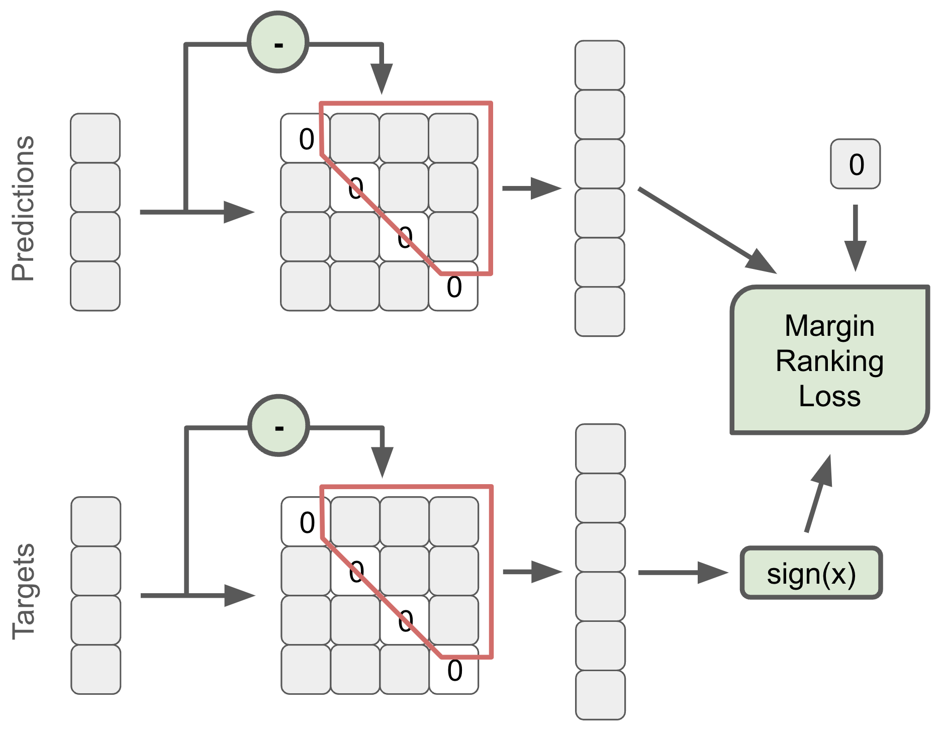\n\n## Remarks on the validation (CV) stability\nWe found Kendall tau on the validation splits extremely unstable for XLA Random and Default since the dataset is relatively small, and there is a significant domain gap between train and validation, and presumably test. Repeats of training results in up to 13 percentage points of difference between outcomes. \n\n## Experiments that did not work\n\n### Data filtration\nSome graphs’ data is badly damaged. For example, `magenta_dynamic` has the following rollout of runtimes vs config ID. In no way can these be measurements from the same graph. \n\n\n\nBelow are other examples where we are unsure about the conditions in which these measurements were performed.\n\n\n\n\nNevertheless, we do not filter out these graphs and others since we could not reliably observe the improvement from their removal due to the earlier mentioned instability of validation Kendall numbers.\n\n### Data recovery\nWe tried to find the damaged data and remove it in an automatic manner by computing block-wise entropy of the runtimes between adjacent blocks. While the detection seems to work visually, we observed a negative impact on the score and did not proceed with this feature.\n\nExample 1:\n\n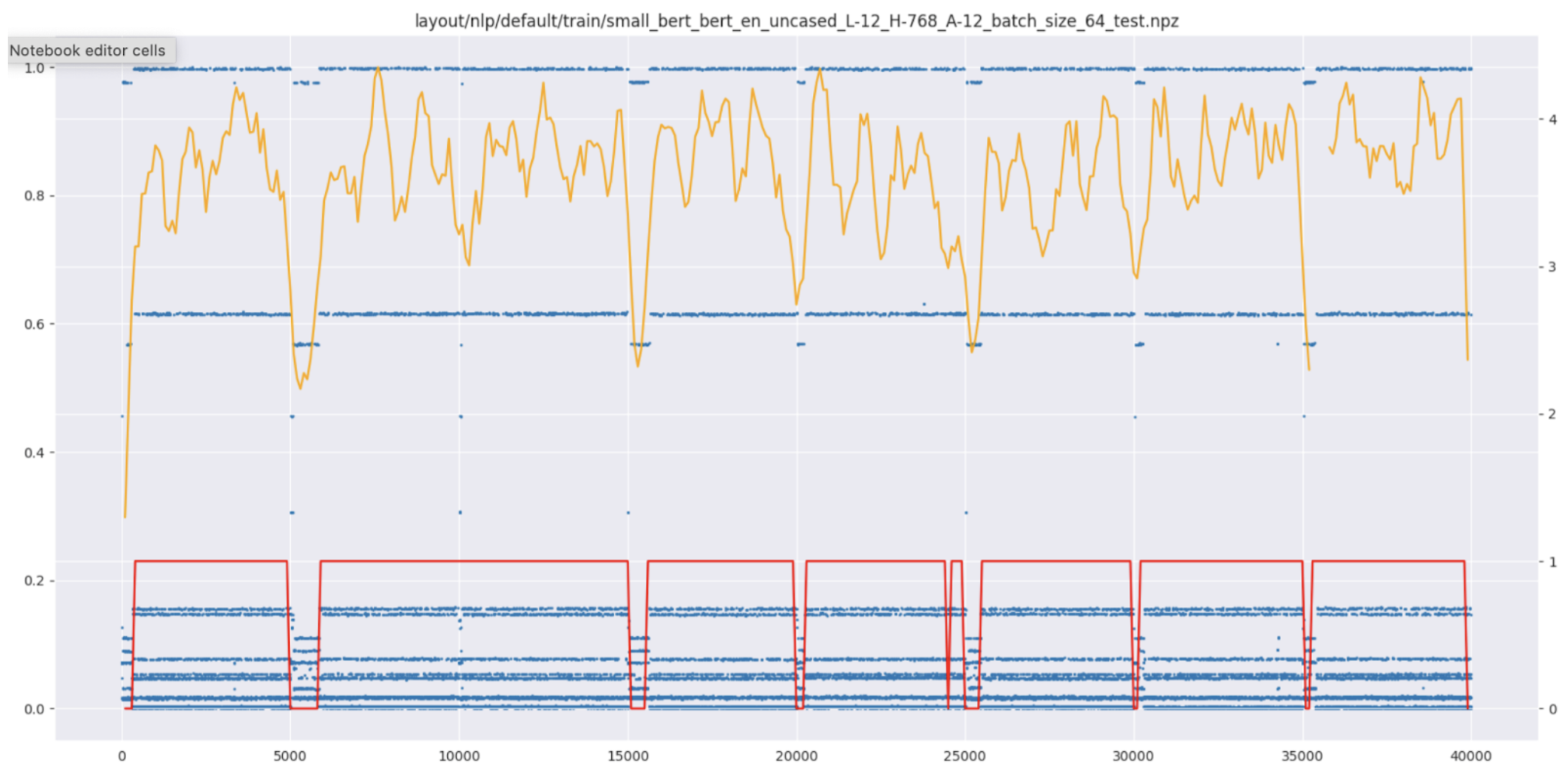\n\nExample 2:\n\n\n\nBefore and after entropy filtration:\n\n\n\n\n### Other experiments we tried that did NOT work:\n1. GATv2Conv, GATv2 backbone, GINEConv,\n2. Dropout,\n3. Training on merged Random and Default - hurts both,\n4. Adding reverse edges,\n5. Online hard negative mining (OHEM) - did not help since train loss is nowhere near zero,\n6. Train blindly on the merged train and valid (trainval),\n7. Train 4 folds and merge by mean latency and by mean reciprocal rank (MRR),\n8. Periodic LR schedule.\n\n## Conclusion\nWe found Google Fast or Slow to be a great competition, and we enjoyed it a lot, along with learning many new things, especially ranking losses.\n\nPartially inspired by this competition, Dmitrii published an article [Ten Patterns and Antipatterns of Deep Learning Experimentation](https://pub.towardsai.net/ten-patterns-and-antipatterns-of-deep-learning-experimentation-e91bb0f6feda) at Towards AI.", "votes": null }, { "id": "2531243", "postDate": "11/20/2023 03:56:55", "content": "Congratulations on securing the 2nd position in this competition. Thanks for sharing the details of your approach with diagram and charts.
", "rawMarkdown": "Congratulations on securing the 2nd position in this competition. Thanks for sharing the details of your approach with diagram and charts.", "votes": null }, { "id": "2532544", "postDate": "11/21/2023 06:27:25", "content": "Thanks for the clear explaination, and congrats for winning
", "rawMarkdown": "Thanks for the clear explaination, and congrats for winning", "votes": null }, { "id": "2532892", "postDate": "11/21/2023 12:28:01", "content": "The code of our solution is available on Github: Fast or Slow by Latenciaga.
", "rawMarkdown": "The code of our solution is available on [Github: Fast or Slow by Latenciaga](https://github.com/Obs01ete/kaggle_latenciaga/tree/master).", "votes": null }, { "id": "2533300", "postDate": "11/21/2023 18:34:56", "content": "Congratulations on winning the second place!
\nWhat does \"For example, magenta_dynamic has the following rollout of runtimes vs config ID. In no way can these be measurements from the same graph\" mean? One hypothesis could be that a small set of config changes affected the runtime a lot, while most of the config changes doesn't.
", "rawMarkdown": "Congratulations on winning the second place!\n\nWhat does \"For example, magenta_dynamic has the following rollout of runtimes vs config ID. In no way can these be measurements from the same graph\" mean? One hypothesis could be that a small set of config changes affected the runtime a lot, while most of the config changes doesn't.", "votes": null }, { "id": "2533885", "postDate": "11/22/2023 09:16:19", "content": "Thanks!
\n\n\nOne hypothesis could be that a small set of config changes affected the runtime a lot, while most of the config changes doesn't.
\n
The point is that, at least for the random search, the distribution of runtimes must be stationary across sample IDs. The distribution is indeed visually stationary for 95% of graphs, the more surprising it was to see non-stationary distributions, which may point to a bug in data collection. Indeed, as you noticed, the distribution may be sophisticated, multimodal, but, in my opinion, it should not be non-stationary for random sampling. It can be non-stationary for genetic algorithms (default sets), but the evolution of the distribution must be smooth, not abrupt, as in the examples in the post.
", "rawMarkdown": "Thanks!\n\n>One hypothesis could be that a small set of config changes affected the runtime a lot, while most of the config changes doesn't.\n\nThe point is that, at least for the random search, the distribution of runtimes must be stationary across sample IDs. The distribution is indeed visually stationary for 95% of graphs, the more surprising it was to see non-stationary distributions, which may point to a bug in data collection. Indeed, as you noticed, the distribution may be sophisticated, multimodal, but, in my opinion, it should not be non-stationary for random sampling. It can be non-stationary for genetic algorithms (default sets), but the evolution of the distribution must be smooth, not abrupt, as in the examples in the post.", "votes": null }, { "id": "2536018", "postDate": "11/23/2023 20:30:30", "content": "This is a very interesting observation. One thing to keep in mind: we generated the data by running either a genetic algorithm search (for default collections) or a random search (for random collections) on 20 independent workers, and we concatenated all the runs together without shuffling for training and validation sets. What you see here is essentially the concatenation of 20 runs.
", "rawMarkdown": "This is a very interesting observation. One thing to keep in mind: we generated the data by running either a genetic algorithm search (for default collections) or a random search (for random collections) on 20 independent workers, and we concatenated all the runs together without shuffling for training and validation sets. What you see here is essentially the concatenation of 20 runs.", "votes": null } ], "comments": [ { "id": 2531243, "author_name": "crsuthikshnkumar", "author_url": "", "post_date": "11/20/2023 03:56:55", "content": "Congratulations on securing the 2nd position in this competition. Thanks for sharing the details of your approach with diagram and charts.
", "votes": null, "replies": [] }, { "id": 2532544, "author_name": "haohantsao", "author_url": "", "post_date": "11/21/2023 06:27:25", "content": "Thanks for the clear explaination, and congrats for winning
", "votes": null, "replies": [] }, { "id": 2532892, "author_name": "dmitriikhizbullin", "author_url": "", "post_date": "11/21/2023 12:28:01", "content": "The code of our solution is available on Github: Fast or Slow by Latenciaga.
", "votes": null, "replies": [] }, { "id": 2533300, "author_name": "zshao9", "author_url": "", "post_date": "11/21/2023 18:34:56", "content": "Congratulations on winning the second place!
\nWhat does \"For example, magenta_dynamic has the following rollout of runtimes vs config ID. In no way can these be measurements from the same graph\" mean? One hypothesis could be that a small set of config changes affected the runtime a lot, while most of the config changes doesn't.
", "votes": null, "replies": [ { "id": 2533885, "author_name": "dmitriikhizbullin", "author_url": "", "post_date": "11/22/2023 09:16:19", "content": "Thanks!
\n\n\nOne hypothesis could be that a small set of config changes affected the runtime a lot, while most of the config changes doesn't.
\n
The point is that, at least for the random search, the distribution of runtimes must be stationary across sample IDs. The distribution is indeed visually stationary for 95% of graphs, the more surprising it was to see non-stationary distributions, which may point to a bug in data collection. Indeed, as you noticed, the distribution may be sophisticated, multimodal, but, in my opinion, it should not be non-stationary for random sampling. It can be non-stationary for genetic algorithms (default sets), but the evolution of the distribution must be smooth, not abrupt, as in the examples in the post.
", "votes": null, "replies": [ { "id": 2536018, "author_name": "mangpophothilimthana", "author_url": "", "post_date": "11/23/2023 20:30:30", "content": "This is a very interesting observation. One thing to keep in mind: we generated the data by running either a genetic algorithm search (for default collections) or a random search (for random collections) on 20 independent workers, and we concatenated all the runs together without shuffling for training and validation sets. What you see here is essentially the concatenation of 20 runs.
", "votes": null, "replies": [] } ] } ] } ], "raw_markdown_by_id": { "2530965": "We express our gratitude to Kaggle as well as Google’s TPU team for organizing this remarkable challenge.\n\nThe code of the solution is available on [Github: Fast or Slow by Latenciaga](https://github.com/Obs01ete/kaggle_latenciaga/tree/master).\n\n## Introduction\nOur implementation is a SageConv-based graph neural network (GNN) operating on whole graphs and trained in PyTorch/PyTorch-Geometric. The GNN was trained with the help of one or two losses, including a novel DiffMat loss, which we will discuss later.\n\n## Dataset preprocessing\nWe preprocess data from all 5 subsets by removing duplicates by config. We discovered that for each graph, several instances of configurations (all node-wise concatenated together for Layout and subgraph for Tile) are identical, while the corresponding runtimes are different with a 0.4% max-to-min difference. We reduce these groups by a minimum. For Layout-XLA, we filtered out all Unet graphs since we identified that `unet_3d.4x4.bf16` is badly corrupted. For the same reason, we removed `mlperf_bert_batch_24_2x2` from Layout-XLA-Default validation to improve the stability of the validation. We identified many other graphs whose data is seemingly corrupted, but we did not filter them out. As a part of preprocessing, we repack the NPZs for Layout so that for each graph, each config+runtime measurement (out of 100k or less) can be loaded from NPZ individually without loading the entire NPZ. With this repacking, thanks to lazy loading, random reads were accelerated 5-10 times, resulting in a similar reduction of training wall clock time, whereas the training became GPU-bound instead of data-loading bound.\n\n## Model\nWe train 5 models from scratch, one for each subset, applying different hyperparameters as summarized in the table below. All GNN layers are SageConv layers with residual connections whenever the number of input and output channels are the same.\n\n| subsets | layers x channels | # parameters |\n| -- | -- | -- |\n| Layout-XLA | 2x64 + 2x128 + 2x256 | 270k |\n| Layout-NLP & Tile | 4x256 + 4x512 | 2.3M |\n\n\n\nThe node types are embedded into 12 dimensions. Node features are compressed with `sign(x)*log(abs(x))` and shaped into 20 dimensions by a linear layer. For Layout, the configs are not transformed; for Tile, the graph configuration is broadcast to all nodes. We apply early fusion by combining the three above into a single feature vector before passing it to GNN layers. Features produced by the GNN layer stack are transformed to one value per node and then sum-reduced to form a single graph-wise prediction. \n\n## Training procedure\n\nWe follow training and validation splits provided by the competition authors. For all 5 subsets, the training was only performed on a training split.\n\nThe batch is organized into 2 levels of hierarchy: the upper level is different graphs, and the lower level is the same graph and different configurations, grouped in microbatches of the same size (also known as slates). This procedure allows applying ranking loss to the group of samples within a microbatch. We found that using some sort of ranking loss is essential for the score. Models trained with a ranking loss (ListMLE, MarginRankingLoss) heavily outperformed element-wise losses (MAPE, etc). \n\n| hyperparameter | Tile subset | Layout- XLA-Random | Layout- XLA-Default | Layout- NLP-Random | Layout- NLP-Default |\n| --- | --- | --- | --- | --- | --- |\n| microbatch size | 10 | 4 | 4 | 10 | 10 |\n| number of microbatches in a batch | 100 | 10 | 10 | 4 | 4 |\n| batch size | 1000 | 40 | 40 | 40 | 40 |\n\n\n\nThe following hyperparameters were set:\n1. Adam/AdamW optimizer,\n2. Learning rate 1e-3,\n3. 400k iterations,\n4. Step learning rate scheduler at 240k, 280k, 320k, and 360k by factor of `1/sqrt(10)`.\n\nTraining time is approximately 20 hours on A100 for each of 5 subsets. No early stopping was employed. All snapshots for submission were taken from the 400k-th iteration.\n\nLosses used for training:\n1. ListMLE for Layout-NLP,\n2. A novel DiffMat loss for Tile,\n3. For Layout-XLA, it is a combination of 2 losses: the DiffMat loss and MAPE loss.\n\nFor ListMLE loss, we used prediction norm-clipping to avoid numerical instability resulting from dividing a big number by a big number. We do not use prediction L2 normalization before ListMLE loss since we find it damages the score.\n\nThe novel DiffMat loss is described with the following algorithm. Within a microbatch, a full antisymmetric matrix of pairwise differences is constructed for the predictions and for the targets. The upper triangular matrix is taken from the difference matrix and flattened. Margin Ranking Loss with a margin of 0.01 is applied between predicted values and zeros. This novel loss, combined with MAPE loss, consistently outperformed ListMLE on XLA.\n\n\n\n## Remarks on the validation (CV) stability\nWe found Kendall tau on the validation splits extremely unstable for XLA Random and Default since the dataset is relatively small, and there is a significant domain gap between train and validation, and presumably test. Repeats of training results in up to 13 percentage points of difference between outcomes. \n\n## Experiments that did not work\n\n### Data filtration\nSome graphs’ data is badly damaged. For example, `magenta_dynamic` has the following rollout of runtimes vs config ID. In no way can these be measurements from the same graph. \n\n\n\nBelow are other examples where we are unsure about the conditions in which these measurements were performed.\n\n\n\n\nNevertheless, we do not filter out these graphs and others since we could not reliably observe the improvement from their removal due to the earlier mentioned instability of validation Kendall numbers.\n\n### Data recovery\nWe tried to find the damaged data and remove it in an automatic manner by computing block-wise entropy of the runtimes between adjacent blocks. While the detection seems to work visually, we observed a negative impact on the score and did not proceed with this feature.\n\nExample 1:\n\n\n\nExample 2:\n\n\n\nBefore and after entropy filtration:\n\n\n\n\n### Other experiments we tried that did NOT work:\n1. GATv2Conv, GATv2 backbone, GINEConv,\n2. Dropout,\n3. Training on merged Random and Default - hurts both,\n4. Adding reverse edges,\n5. Online hard negative mining (OHEM) - did not help since train loss is nowhere near zero,\n6. Train blindly on the merged train and valid (trainval),\n7. Train 4 folds and merge by mean latency and by mean reciprocal rank (MRR),\n8. Periodic LR schedule.\n\n## Conclusion\nWe found Google Fast or Slow to be a great competition, and we enjoyed it a lot, along with learning many new things, especially ranking losses.\n\nPartially inspired by this competition, Dmitrii published an article [Ten Patterns and Antipatterns of Deep Learning Experimentation](https://pub.towardsai.net/ten-patterns-and-antipatterns-of-deep-learning-experimentation-e91bb0f6feda) at Towards AI.", "2531243": "Congratulations on securing the 2nd position in this competition. Thanks for sharing the details of your approach with diagram and charts.", "2532544": "Thanks for the clear explaination, and congrats for winning", "2532892": "The code of our solution is available on [Github: Fast or Slow by Latenciaga](https://github.com/Obs01ete/kaggle_latenciaga/tree/master).", "2533300": "Congratulations on winning the second place!\n\nWhat does \"For example, magenta_dynamic has the following rollout of runtimes vs config ID. In no way can these be measurements from the same graph\" mean? One hypothesis could be that a small set of config changes affected the runtime a lot, while most of the config changes doesn't.", "2533885": "Thanks!\n\n>One hypothesis could be that a small set of config changes affected the runtime a lot, while most of the config changes doesn't.\n\nThe point is that, at least for the random search, the distribution of runtimes must be stationary across sample IDs. The distribution is indeed visually stationary for 95% of graphs, the more surprising it was to see non-stationary distributions, which may point to a bug in data collection. Indeed, as you noticed, the distribution may be sophisticated, multimodal, but, in my opinion, it should not be non-stationary for random sampling. It can be non-stationary for genetic algorithms (default sets), but the evolution of the distribution must be smooth, not abrupt, as in the examples in the post.", "2536018": "This is a very interesting observation. One thing to keep in mind: we generated the data by running either a genetic algorithm search (for default collections) or a random search (for random collections) on 20 independent workers, and we concatenated all the runs together without shuffling for training and validation sets. What you see here is essentially the concatenation of 20 runs." }, "source": "meta" }