
Congratulations to everyone on finishing the Fast or Slow competition and a big thanks to my amazing teammate @drhabib. After the competition announcement, we were quite excited about seeing quite an interesting problem considered in it. However, a more detailed look has disclosed that the evaluation is performed only on a few graphs, i.e. the evaluation may be very unstable, and the risk of massive two-digit shakeup was significant (I'm curious if organizers performed a config-based split instead of graph one to avoid it?). So we considered this competition as a lottery and spent here only ~1.5 weeks while working on another competition.
\nThe approaches frequently considered in the literature are often based either on early or late fusion, i.e. injection of the configuration input is performed either at the very beginning or after collapsing the graph representation into a single embedding vector. However, the first one struggles with computational inefficiency because the computation must be performed for each configuration independently, which results in issues when thousands of configurations are considered with graphs containing tens of thousands of nodes. Meanwhile, the late fusion method loses the node-specific information at the moment of fusion after collapsing all nodes into a single embedding vector, i.e. the model may have a difficult time assigning a particular configuration to the corresponding nodes.
\nThe key idea of our approach is using the intermediate fusion that provides a good balance between computational efficiency and the expressiveness of the graph representation at the moment of fusion with configuration input. Therefore, we may perform training with 1000s configurations and huge (graphs up to 10^4 nodes) at the same time without a significant overhead. The use of a large number of configurations in each batch is critical for sequence ranking losses like listMLE. Meanwhile, at the moment of fusion, the nodes do not collapse into a single embedding vector, and a particular configuration may be directly associated with the nodes.
\nSome of the node features describe the dimensions of data and kernels, and the product of the dimensions may be as large as 10^6. It is not really acceptable for models, and we simply took a log of input features + 3 to have comparable scales. In our experiments, we also tried to extract additional 29 graph features by customizing the organizer's code but got comparable results to just using the base 140 features.
\nIn the layout pipeline instead of storing everything in the RAM, which may be quite large in comparison to tile data, we loaded only graph features (several GB only). Meanwhile, the configs were sampled in chunks of 1000 and loaded during training in a just-in-time manner instead of loading all configurations and using only 1000 of them. It has eliminated the data loading bottleneck.
\nOur model is based on transformers adapted to work effectively with graph data on consumer-grade hardware.
\n(Tile) Specifically, the tile model uses a sequence of residual graph blocks, enabling the creation of the local neighborhood representation, before global mixing with self-attention blocks followed by node information retrieval for particular configurations with cross-attention transformer blocks. With this setup training of the model reaching 0.97+ slowdown metric takes under 1 min. The LB of our tile-only model is 0.196 at private and 0.197 at public out of 0.2. The combination of different folds gave 0.196 and 0.198 at private and public LB.
\n(Layout) In the layout model, we must replace standard dot product attention with multi-head linear attention, which has linear complexity on the number of tokens. This attention enables a global receptive field within the entire 10^4 node graph while being relatively computationally cheap enabling running 12 block transformer on GPUs like 4090 or A6000. We replaced the ReLU nonlinearity in the attention with a more robust ELU+1 function. We do not use SLA in the tile model because of difficulties with masking padding tokens. The MLP part of the transformer blocks, meanwhile, is replaced with graph networks, which enable local mixing of features between neighboring nodes. We considered APPNP, SAGE, GAT, GPRGNN graph modules, with APPNP getting slightly better results. We considered both, unidirectional and bidirectional graph models. In one set of experiments, we also considered 4 and 6 layers DiFFormer model. The graph transformer is followed by pooling of configurable nodes, concatenation of them with the corresponding configurations and mixing with MLP, and finally by global pooling among all configurable nodes and prediction of the overall ranking. The models are illustrated in the plot at the beginning of the post.
\nWith the intermediate fusion approach even relatively wide (n=256) and deep (up to 12 layers) models are very fast, taking just a few seconds per epoch on tile setup, a few minutes per epoch with XLA layouts, and 30 min to 1 hour for NLP layouts while using up to 1000 configurations simultaneously. The convergence takes ~5 epochs for tile models and 16 epochs for layout ones.
\nWe used standard for transformers AdamW optimizer, cosine annealing with lr=5e-4, and wd of 1e-2. The training is performed for 5 epochs for tile and for 16 epochs for layout models. In some runs, we used EMA average of weights and gradient accumulation. We used listMLE as the loss function, which was possible because we considered ~1000 configurations for a given graph in each batch.
\nSince XLA and NLP graphs exhibit a drastic difference in graph size we decided to split them into two separate sets of models trained independently. Specifically, XLA graphs are huge (VRAM hungry) and the number of configs is low. While NLP graphs are quite smaller with a huge number of configs (i.e. longer training). So we could train XLA models with 256 configs per graph on 24 GB VRAM GPUs and 256-1000 configs on 48 GB VRAM GPUs. While NLP models are easily trained with 1000 configs per graph taking less than 24 GB VRAM.
\nRunning experiments we quickly realized that evaluation on eval set is not stable, and nearly all considered setups achieved statistically insignificant differences in comparison to reruning the same setup with a different seed. It did not allow us to assess the real improvement of models under different setups and report the ablation study.
\nWe set an 11-fold split scheme (val set + 10-fold split of train set) to enable sufficient precision of evaluation needed to distinguish small performance differences in the considered setups. However, given only ~1 week remaining for us in the competition and 8-16 hours per fold total training time for NLP layouts, we did not proceed much further with that and ran just a few folds for diversity in several experiments.
\nOur main strategy in this competition, since we could not reliably assess the performance, was running as many configurations as possible and mixing them together to mitigate the effect of the possible shakeup. We composed 10-20 different configurations for XLA and NLP models. This setup got 0.712 and 0.696 at public and private LB.
\nIn addition, we selected our best public LB submission, which consists of 2 APPNP XLA models and 2 DIFFormer NLP models. It reaches 0.721 at public and 0.703 at private LB. A very surprising result for us.
\nOur best lucky private LB sub meanwhile, is 0.706 and 0.715 at public and private LB. In this sub we used APPNP models with gated units instead of residual sum.
Congratulations to everyone on finishing the Fast or Slow competition and a big thanks to my amazing teammate @drhabib. After the competition announcement, we were quite excited about seeing quite an interesting problem considered in it. However, a more detailed look has disclosed that the evaluation is performed only on a few graphs, i.e. the evaluation may be very unstable, and the risk of massive two-digit shakeup was significant (I'm curious if organizers performed a config-based split instead of graph one to avoid it?). So we considered this competition as a lottery and spent here only ~1.5 weeks while working on another competition.
\nThe approaches frequently considered in the literature are often based either on early or late fusion, i.e. injection of the configuration input is performed either at the very beginning or after collapsing the graph representation into a single embedding vector. However, the first one struggles with computational inefficiency because the computation must be performed for each configuration independently, which results in issues when thousands of configurations are considered with graphs containing tens of thousands of nodes. Meanwhile, the late fusion method loses the node-specific information at the moment of fusion after collapsing all nodes into a single embedding vector, i.e. the model may have a difficult time assigning a particular configuration to the corresponding nodes.
\nThe key idea of our approach is using the intermediate fusion that provides a good balance between computational efficiency and the expressiveness of the graph representation at the moment of fusion with configuration input. Therefore, we may perform training with 1000s configurations and huge (graphs up to 10^4 nodes) at the same time without a significant overhead. The use of a large number of configurations in each batch is critical for sequence ranking losses like listMLE. Meanwhile, at the moment of fusion, the nodes do not collapse into a single embedding vector, and a particular configuration may be directly associated with the nodes.
\nSome of the node features describe the dimensions of data and kernels, and the product of the dimensions may be as large as 10^6. It is not really acceptable for models, and we simply took a log of input features + 3 to have comparable scales. In our experiments, we also tried to extract additional 29 graph features by customizing the organizer's code but got comparable results to just using the base 140 features.
\nIn the layout pipeline instead of storing everything in the RAM, which may be quite large in comparison to tile data, we loaded only graph features (several GB only). Meanwhile, the configs were sampled in chunks of 1000 and loaded during training in a just-in-time manner instead of loading all configurations and using only 1000 of them. It has eliminated the data loading bottleneck.
\nOur model is based on transformers adapted to work effectively with graph data on consumer-grade hardware.
\n(Tile) Specifically, the tile model uses a sequence of residual graph blocks, enabling the creation of the local neighborhood representation, before global mixing with self-attention blocks followed by node information retrieval for particular configurations with cross-attention transformer blocks. With this setup training of the model reaching 0.97+ slowdown metric takes under 1 min. The LB of our tile-only model is 0.196 at private and 0.197 at public out of 0.2. The combination of different folds gave 0.196 and 0.198 at private and public LB.
\n(Layout) In the layout model, we must replace standard dot product attention with multi-head linear attention, which has linear complexity on the number of tokens. This attention enables a global receptive field within the entire 10^4 node graph while being relatively computationally cheap enabling running 12 block transformer on GPUs like 4090 or A6000. We replaced the ReLU nonlinearity in the attention with a more robust ELU+1 function. We do not use SLA in the tile model because of difficulties with masking padding tokens. The MLP part of the transformer blocks, meanwhile, is replaced with graph networks, which enable local mixing of features between neighboring nodes. We considered APPNP, SAGE, GAT, GPRGNN graph modules, with APPNP getting slightly better results. We considered both, unidirectional and bidirectional graph models. In one set of experiments, we also considered 4 and 6 layers DiFFormer model. The graph transformer is followed by pooling of configurable nodes, concatenation of them with the corresponding configurations and mixing with MLP, and finally by global pooling among all configurable nodes and prediction of the overall ranking. The models are illustrated in the plot at the beginning of the post.
\nWith the intermediate fusion approach even relatively wide (n=256) and deep (up to 12 layers) models are very fast, taking just a few seconds per epoch on tile setup, a few minutes per epoch with XLA layouts, and 30 min to 1 hour for NLP layouts while using up to 1000 configurations simultaneously. The convergence takes ~5 epochs for tile models and 16 epochs for layout ones.
\nWe used standard for transformers AdamW optimizer, cosine annealing with lr=5e-4, and wd of 1e-2. The training is performed for 5 epochs for tile and for 16 epochs for layout models. In some runs, we used EMA average of weights and gradient accumulation. We used listMLE as the loss function, which was possible because we considered ~1000 configurations for a given graph in each batch.
\nSince XLA and NLP graphs exhibit a drastic difference in graph size we decided to split them into two separate sets of models trained independently. Specifically, XLA graphs are huge (VRAM hungry) and the number of configs is low. While NLP graphs are quite smaller with a huge number of configs (i.e. longer training). So we could train XLA models with 256 configs per graph on 24 GB VRAM GPUs and 256-1000 configs on 48 GB VRAM GPUs. While NLP models are easily trained with 1000 configs per graph taking less than 24 GB VRAM.
\nRunning experiments we quickly realized that evaluation on eval set is not stable, and nearly all considered setups achieved statistically insignificant differences in comparison to reruning the same setup with a different seed. It did not allow us to assess the real improvement of models under different setups and report the ablation study.
\nWe set an 11-fold split scheme (val set + 10-fold split of train set) to enable sufficient precision of evaluation needed to distinguish small performance differences in the considered setups. However, given only ~1 week remaining for us in the competition and 8-16 hours per fold total training time for NLP layouts, we did not proceed much further with that and ran just a few folds for diversity in several experiments.
\nOur main strategy in this competition, since we could not reliably assess the performance, was running as many configurations as possible and mixing them together to mitigate the effect of the possible shakeup. We composed 10-20 different configurations for XLA and NLP models. This setup got 0.712 and 0.696 at public and private LB.
\nIn addition, we selected our best public LB submission, which consists of 2 APPNP XLA models and 2 DIFFormer NLP models. It reaches 0.721 at public and 0.703 at private LB. A very surprising result for us.
\nOur best lucky private LB sub meanwhile, is 0.706 and 0.715 at public and private LB. In this sub we used APPNP models with gated units instead of residual sum.
Congratulations on achieving 10th position. Thanks for sharing details of your solution.
", "rawMarkdown": "Congratulations on achieving 10th position. Thanks for sharing details of your solution.", "votes": null } ], "comments": [ { "id": 2529891, "author_name": "crsuthikshnkumar", "author_url": "", "post_date": "11/18/2023 16:19:00", "content": "Congratulations on achieving 10th position. Thanks for sharing details of your solution.
", "votes": null, "replies": [] } ], "raw_markdown_by_id": { "2529394": "## Summary\n1. Intermediate config fusion\n2. Graph transformer based solution\n3. The best lucky model got 0.715 at private LB\n\n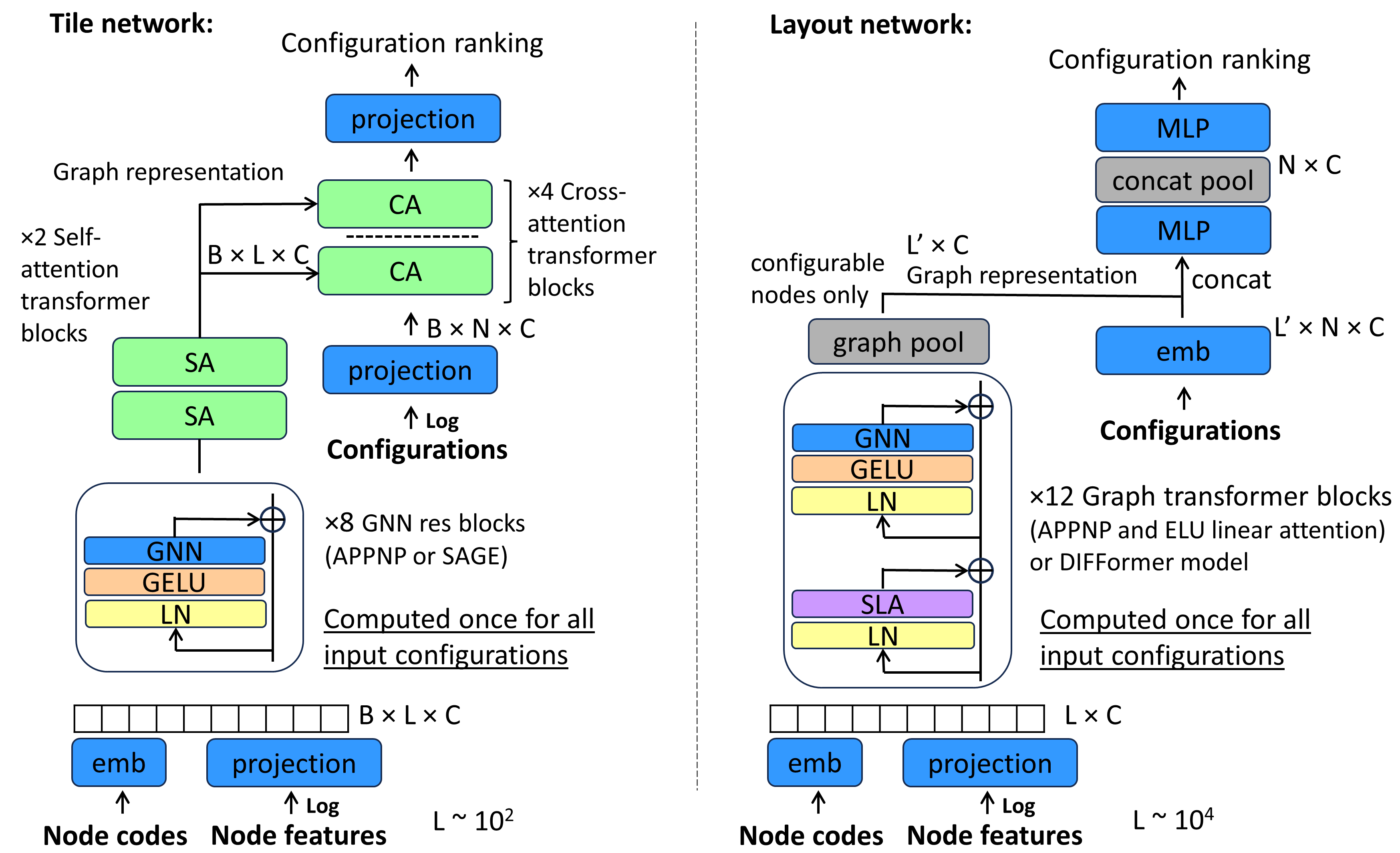\n\nCongratulations to everyone on finishing the Fast or Slow competition and a big thanks to my amazing teammate @drhabib. After the competition announcement, we were quite excited about seeing quite an interesting problem considered in it. However, a more detailed look has disclosed that the evaluation is performed only on a few graphs, i.e. the evaluation may be very unstable, and the risk of massive two-digit shakeup was significant (I'm curious if organizers performed a config-based split instead of graph one to avoid it?). So we considered this competition as a lottery and spent here only ~1.5 weeks while working on another competition.\n\n## Details\n\nThe approaches frequently considered in [the literature](https://arxiv.org/pdf/2008.01040.pdf) are often based either on early or late fusion, i.e. injection of the configuration input is performed either at the very beginning or after collapsing the graph representation into a single embedding vector. However, the first one struggles with computational inefficiency because the computation must be performed for each configuration independently, which results in issues when thousands of configurations are considered with graphs containing tens of thousands of nodes. Meanwhile, the late fusion method loses the node-specific information at the moment of fusion after collapsing all nodes into a single embedding vector, i.e. the model may have a difficult time assigning a particular configuration to the corresponding nodes. \n\n**The key idea of our approach is using the intermediate fusion** that provides **a good balance between computational efficiency and the expressiveness of the graph representation at the moment of fusion with configuration input**. Therefore, we may perform training with 1000s configurations and huge (graphs up to 10^4 nodes) at the same time without a significant overhead. The use of a large number of configurations in each batch is critical for sequence ranking losses like listMLE. Meanwhile, at the moment of fusion, the nodes do not collapse into a single embedding vector, and a particular configuration may be directly associated with the nodes.\n\n### Data\nSome of the node features describe the dimensions of data and kernels, and the product of the dimensions may be as large as 10^6. It is not really acceptable for models, and we simply took a log of input features + 3 to have comparable scales. In our experiments, we also tried to extract additional 29 graph features by customizing the organizer's code but got comparable results to just using the base 140 features.\n\nIn the layout pipeline instead of storing everything in the RAM, which may be quite large in comparison to tile data, we loaded only graph features (several GB only). Meanwhile, the configs were sampled in chunks of 1000 and loaded during training in a just-in-time manner instead of loading all configurations and using only 1000 of them. It has eliminated the data loading bottleneck.\n\n### Model\n**Our model is based on transformers adapted to work effectively with graph data on consumer-grade hardware.** \n\n(Tile) Specifically, the tile model uses a sequence of residual graph blocks, enabling the creation of the local neighborhood representation, before global mixing with self-attention blocks followed by node information retrieval for particular configurations with cross-attention transformer blocks. With this setup training of the model reaching 0.97+ slowdown metric takes under 1 min. The LB of our tile-only model is 0.196 at private and 0.197 at public out of 0.2. The combination of different folds gave 0.196 and 0.198 at private and public LB.\n\n(Layout) In the layout model, we must replace standard dot product attention with multi-head [linear attention](https://arxiv.org/pdf/2205.14756.pdf), which has linear complexity on the number of tokens. This attention enables a global receptive field within the entire 10^4 node graph while being relatively computationally cheap enabling running 12 block transformer on GPUs like 4090 or A6000. We replaced the ReLU nonlinearity in the attention with a more robust ELU+1 function. We do not use SLA in the tile model because of difficulties with masking padding tokens. The MLP part of the transformer blocks, meanwhile, is replaced with graph networks, which enable local mixing of features between neighboring nodes. We considered APPNP, SAGE, GAT, GPRGNN graph modules, with APPNP getting slightly better results. We considered both, unidirectional and bidirectional graph models. In one set of experiments, we also considered 4 and 6 layers [DiFFormer model](https://arxiv.org/pdf/2301.09474.pdf). The graph transformer is followed by pooling of configurable nodes, concatenation of them with the corresponding configurations and mixing with MLP, and finally by global pooling among all configurable nodes and prediction of the overall ranking. The models are illustrated in the plot at the beginning of the post.\n\nWith the intermediate fusion approach even relatively wide (n=256) and deep (up to 12 layers) models are very fast, taking just a few seconds per epoch on tile setup, a few minutes per epoch with XLA layouts, and 30 min to 1 hour for NLP layouts while using up to 1000 configurations simultaneously. The convergence takes ~5 epochs for tile models and 16 epochs for layout ones.\n\n### Training\nWe used standard for transformers AdamW optimizer, cosine annealing with lr=5e-4, and wd of 1e-2. The training is performed for 5 epochs for tile and for 16 epochs for layout models. In some runs, we used EMA average of weights and gradient accumulation. We used listMLE as the loss function, which was possible because we considered ~1000 configurations for a given graph in each batch.\n\nSince XLA and NLP graphs exhibit a drastic difference in graph size we decided to split them into two separate sets of models trained independently. Specifically, XLA graphs are huge (VRAM hungry) and the number of configs is low. While NLP graphs are quite smaller with a huge number of configs (i.e. longer training). So we could train XLA models with 256 configs per graph on 24 GB VRAM GPUs and 256-1000 configs on 48 GB VRAM GPUs. While NLP models are easily trained with 1000 configs per graph taking less than 24 GB VRAM.\n\n### Evaluation\n**Running experiments we quickly realized that evaluation on eval set is not stable, and nearly all considered setups achieved statistically insignificant differences in comparison to reruning the same setup with a different seed.** It did not allow us to assess the real improvement of models under different setups and report the ablation study. \n\nWe set an 11-fold split scheme (val set + 10-fold split of train set) to enable sufficient precision of evaluation needed to distinguish small performance differences in the considered setups. However, given only ~1 week remaining for us in the competition and 8-16 hours per fold total training time for NLP layouts, we did not proceed much further with that and ran just a few folds for diversity in several experiments. \n\n### Final model\nOur main strategy in this competition, since we could not reliably assess the performance, was running as many configurations as possible and mixing them together to mitigate the effect of the possible shakeup. We composed 10-20 different configurations for XLA and NLP models. This setup got 0.712 and 0.696 at public and private LB.\nIn addition, we selected our best public LB submission, which consists of 2 APPNP XLA models and 2 DIFFormer NLP models. It reaches 0.721 at public and 0.703 at private LB. A very surprising result for us. \nOur best lucky private LB sub meanwhile, is 0.706 and 0.715 at public and private LB. In this sub we used APPNP models with gated units instead of residual sum.", "2529891": "Congratulations on achieving 10th position. Thanks for sharing details of your solution." }, "source": "meta" }