
Many thanks to the competition host and Kaggle for another engaging challenge—and congratulations to all the participants!
\nAs always, I had a great time learning throughout the competition. It was indeed a crazy race to the deadline for me, filled with many emotions until the very end. I am really happy to share a few thoughts on my solution here.
\nChangelogs:
\n
A 2D UNet model was trained to predict 57 \"feature-rich\" keypoints and 43*55=2365 grid keypoints, as shown in the figure below.

I obtained the exact coordinates for all 2,422 keypoints by inspecting the ecg-image-kit source code. The \"main\" keypoints were heuristically selected, typically around the calibration pulses, splitting ticks, and lead names, which I consider to have rich local features.
\n\n\nNote: I ignored some near-border grid keypoints since they could confuse the model. However, this caused many headaches in the subsequent registering stage. Perhaps keeping all
\n44*57instead of just42*55keypoints would have been a better choice :D
I use one of the SOTA opensource dense matching model MINIMA-RoMa to obtain very accurate initial pseudo-labeled keypoints. This involved simply matching the type 0001 image to each image in the training set.
\n
Note that I did not perform matching followed by Homography matrix estimation to warp reference keypoints into current image's space, because it generates wrong keypoint coordinates if the scene is non-planar or if local distortion is heavy. Instead, for modern dense matching models (LoFTR, RoMA, etc.), we can resample/interpolate the predicted warping flow at arbitrary coordinates in an image to estimate the sub-pixel level matched keypoint coordinates on the remaining one.
\nYou can try more recent SOTA methods on Image Matching very quickly using this awesome demo: https://huggingface.co/spaces/Realcat/image-matching-webui
\nA 2D UNet model was trained to predict a 58-channel output heatmap:
\nsigma=2 px relative to the standard reference image (type 0001, 1700x2200), adaptively scaled based on the current image's scale (relative to the reference).sigma=2px, similar to the setting above. \nVisualization of an augmented train samples, left to right: augmented image, visualization of 2nd-58th heatmap channels, first channel encode grid points, overlayed visualization
The model was trained end-to-end using multi-task losses. Despite the fact that the network can be trained using just BCE loss, I used BCE for the first channel and Channel-Masked JSD (Jensen-Shannon Divergence) for the remaining 57 channels. Each of the 57 channels encodes only a single keypoint Gaussian heatmap; the spatial distribution has 0 peaks (when the keypoint is outside the image) or 1 peak (unimodal), unlike the multiple peaks (multimodal) distribution of the first channel. Thus, a spatial distribution-based loss (JSD, KLDiv, CE) provides better inductive bias/regularization compared to BCE. Using JSD allows for much faster convergence, which I have confirmed in almost every experiment/project I have finished in the past.
\nAdditionally, scaling the image size proved better than scaling the model size. We already know that the pattern/context is not very hard to predict for a model in this particular task (I found MaxVit, a hybrid CNN-Transformer, did not outperform a ConvNeXT-small with a much more limited receptive field). Therefore, local pattern recognition is sufficient, allowing the use of a CNN-only architecture which is much easier to scale to larger image sizes. Larger image size is critically important to obtain a fine-grained heatmap with less sub-pixel error. Furthermore, if the ROI in the test image is much smaller than the captured image (e.g., the camera is far from the object), a longest resize + padding transform will destroy details, so resolution must be prioritized.
I measured a keypoint metric similar to AP@0.5-0.95 for grid keypoints and Accuracy@0.5-0.95 for the 57 main keypoints to track the best model. The final config used to train the 5-fold models was:
3x2048x2048 image size, longest resize + padding with bicubic interpolation.58x2048x2048.[384, 256, 128, 64] channels. Tried other options such as PixelShuffle-based decoder, but they did not outperform the baseline.64 -> 128 -> 58 with GELU and LayerNorm.1e-4, Cosine scheduler.After the heatmap model was trained, I finetuned each fold model using an additional loss to achieve sub-pixel accuracy on main keypoint predictions: MSELoss on DSNT prediction and groundtruth coordinates of shape (57, 2), resulting in 3 total losses.
I train 5 models on 5 folds to obtain the OOF predictions, decode, then some postprocessing logics defined in the subsequent section Keypoint Registration was applied. This process is treated as a denoising process, where I hope model will learn the average/correct truth and skipping the small amount of noises in the initial pseudo label by MINIMA-RoMa. After 1 round, prediction is good enough and this round 1 pseudo label was used to train final keypoint estimation models for submission.
\nAfter obtaining the heatmap from the previous stage, the next task is to decode the heatmap into discrete keypoints and register/order them correctly. The following logic was applied sequentially:
\nargmax over the 2D spatial heatmap for each of the 2nd-58th output channels. This way, we already know the correct keypoint order. We can use a confidence score to determine if a keypoint is outside the image region, but it's not trustworthy since the model is not supervised on \"out-of-region\" keypoints (channel-masked in JSD loss). Fortunately, subsequent stages are robust enough to handle WRONG predictions of outside-image keypoints.(5, 57, 2) decoded main keypoints. Simply flatten to (285, 2), using those \"nearly duplicated\" keypoints to estimate the Homography Transformation matrix H (strong assumption that it's an Affine transform) and the relative scale from the standard reference image (type 0001) to the current images. RANSAC is robust to outliers, so wrong predictions/noise from the previous stage are filtered. \nThis GIF describes how the keypoints registering algorithm worked step by step
Given the original images and 2,422 keypoints estimated from the previous stage, we can proceed to cropping. All images use the same reference template (type 0001), so it's easier to crop out an arbitrary region of interest, predefined using coordinates in the reference template. Several cropping methods were tested:
\ncv.getPerspectiveTransform locally -> compute flow map -> resample using cv2.remap (or F.grid_sample or scipy.ndimage.map_coordinates).scipy.interpolate.RectBivariateSpline.cv2.findHomography to find a local Homography on K=16 nearby keypoints instead of just K=4 as in (2).
Method (4) performed the best, since it is not too global as in (1) but keeps the \"locality\" property enough to well-handle local distortion, without being too strictly local and sensitive to grid keypoint estimation errors as in (2).
\n \nMisalignment due to local distortion using method (1) - see the sharp peaks, but much better results were obtained using method (4)
Given a warped crop of each lead, another UNet was trained to predict a 2D heatmap of the lead waveform.\nI think the encoding scheme (codec) is important here. For each lead, I crop out the lead image region slightly wider on both the left and right to prevent slight rectification errors from the previous stage destroying the signal needed for prediction. That is, even if the crop is left-shifted or right-shifted by a small number of pixels, the rendered waveform is still fully included in the image, thus can be recovered by a good model.
\n
As for the heatmap, I render it in a column-independent way. Each column is an unnormalized 1D-Gaussian heatmap with 1 peak (mu) at the groundtruth value, and a std (sigma) value is fixed or adaptively changed based on the waveform itself. So, each column always represents a probability distribution with a single peak. This codec scheme is \"nearly lossless\", i.e., it maintains a very high SNR during the encoding and decoding back (recomputing expectation from a probability density function) operation.
\n \nUNet architecture with dual-encoder. A VGG19 encodes finegrained features at stride 1/2/4 while another coarse encoder of either CoaT Lite Medium or ConvNeXT Large aggregate global/nearby information, better handles occlusion or captures long-range dependencies
Indeed, I had not trained this final architecture before; I just trained it once on all data to get a single checkpoint to submitted just before by the deadline. The hyperparameters were selected based on heuristics and previous experiments, in which I combined everything \"that should work\" into the final trial. All previous experiments did not introduce the VGG19 fine-grained/high-resolution encoder, but rather relied on a simpler baseline:
\n512x512, GT waveform is resampled to a fixed length of 500, GT heatmap has shape (1, 512, 512) where the center region (1, 512, 500) actually encodes the GT waveform.K=4).(1, 512, 512).F.softmax(dim=2) on predicted tensor of shape NCHW).Some key insights:
\nWarping interpolation mode matters to prevent losing very fine-grained details: cv2.INTER_LANCZOS4 performed the best and was used in almost all experiments.
Heatmap Gaussian sigma is 2px relative to the reference template image 0001.
Adaptive sigma scale: The rationale behind this is that some parts of the waveform are harder to predict than others, e.g., sharp peaks where the magnitude significantly changes in a short time, resulting in a \"near straight line\" parallel to the mV axis. A simple method was applied which increases the sigma value for waveform values where the local standard deviation is large. Its effectiveness was validated by an improvement in local CV.
\nSIGMA, ADAPTIVE_FACTOR = 2, 0.4\nlocal_abs_diff = 0.5 * (np.abs(arr - np.r_[arr[0], arr[:-1]]) + np.abs(arr - np.r_[arr[1:], arr[-1]]))\n# 3-sigma rule: if > 3*sigma, start using scale >= 1\nadaptive_sigma_arr = SIGMA + ADAPTIVE_FACTOR * np.maximum(local_abs_diff - 3 * SIGMA, 0) / 3\n
Column-wise JSD loss was used. In short: JSD > CE >> BCE.
UNet Decoder: The final model uses 6 UNet Decoder blocks, decoder channels [256,192,160,128,96,64] corresponding to stride 64 -> 1 with LayerNorm and GELU activation. Performance scales better with the number of parameters. A higher number of channels in the high-resolution feature map is needed to preserve fine-grained texture details, but this also increases memory heavily. For the upscale type, a PixelShuffle-based Decoder was tried but didn't outperform the traditional F.interpolate(). Deformable Convolution (v2 or v4) was also tried as a drop-in replacement for traditional nn.Conv2d and showed better performance, but was not used due to slower runtime; I argued that gains came from the increased parameter count instead.
Resolution matters: The use of an input image size of 1024 is critical to keep texture details, bringing significant gains over 512. Before this, I tested if the gain came from higher input resolution or higher output resolution by sweeping over some modeling configs:
\nMain encoder: CoAT and ConvNext-large were used. The two architectures show different characteristics. CoAT tends to be slightly better on noisy and occluded image types, possibly due to a larger receptive field and more input-dynamic nature, hence it can use nearby information to guess what is under occlusion. Meanwhile, ConvNext is better at locality and extracting fine-grained features, hence better SNR on good and high-resolution images such as phone photos.
\n
Comparison is unfair due to different image sizes (1024 vs 512), but still shows some characteristics of each architecture: pure-CNN vs Hybrid CNN-Transformer.
The \"fine\" encoder: VGG19 encoder to extract feature maps at stride 1/2/4. We know that this task strongly benefits from low-level feature maps and high resolution, and VGG is one of the very few architectures which outputs a stride 1 feature map by default. VGG is also used in RoMA and proved to be better than ResNet-like architectures in extracting fine-grained local features. I used vgg19.tv_in1k which does not use BatchNorm, inspired by Image Super Resolution literature (EDSR)
The blank template: I use ecg-image-kit to render an empty image without any lead waveform, acting as a blank template with just grids, calibration pulses, separation ticks, and lead names. Each lead crop was concatenated with the corresponding grayscale blank template, resulting in a 4-channel image to be passed to the 2D UNet model, instead of the original 3-channel RGB image. I hypothesize the template is useful for the model to better learn the local correlation between the rectified image and the standard grid template (aligned perfectly with groundtruth heatmap), allowing it to internally learn to alignment accordingly. It also reduces the complexity of learning lead-specific grid layouts, hence faster convergence
\n
Augmentation: The key augmentation was to add a small amount of noise (following a truncated normal distribution with sigma=0.4px) into the detected grid keypoints before the lead cropping procedure (using local Piecewise Homography transform (2)). This mimics real-life errors since the keypoint detector's prediction is not perfectly accurate. I found not much gain from usual augmentations like ColorJitter, BrightnessContrast, Grayscale, or very small Affine/Perspective transforms, so I set these augmentation probabilities to a small value p=0.1
Training: AdamW optimizer, Cosine LR scheduler, gradient clipping by norm of 1.0, and models are trained for about 70K steps with an effective batch size of 8 (batch size 2, gradient accumulation 4)
Model EMA with decay=0.999
Details in the training code repo
\nThere are 69 rotated image in the training set. Not sure how many in test set, and wrong orientation will affect the keypoints detection stage. So I train a simple model to correct/standardize image orientation.
\nFor each image, we can get the exact rotation angle relative to the standard reference image using Homography H. I simply trained a efficientvit_b2.r224_in1k to jointly predict one of 4 possible rotations 0/90/180/270 degrees (classification task) and the exact rotation angle encoded by sine/cosine (regression task). During training, heavy augmentation was applied to ensure the trained model would be robust on the unseen private test set. Of course, the training task is just too easy, so the validation accuracy is 100% and angle MAE is just around 1.1 degrees.
\nI wrote the inference code and submitted it near the deadline; everything was a mess and aweful on that last day..\nAll submissions include the inference pipeline for a single Image Rotation/Orientation model and 5-fold keypoint detection models.
\nThe first 4 submissions all estimate lead waveforms using a single model without ensemble, and prediction dynamic was also limited to the range [-3.2, 3.2] due to the nature of the heatmap codec. Interestingly, just scaling the image size did not work—my model did not generalize well to the new input size. That is, training on input size [512, 512] (which can encode [-3.2, 3.2] waveforms) and then inferencing on input size [1024, 512] (which can encode [-6.4, 6.4] waveforms) resulted in very bad SNR.
4 single models were submitted:
\n[1024, 1024], output heatmap of size [1024, 1024] (first time training, no validation).[1024, 1024], output heatmap of size [1024, 1024] (first time training, no validation).[512, 512], output heatmap of size [512, 512] (best learning rate is known).[1024, 1024], output heatmap of size [1024, 1024] (best learning rate is known).The final submission:
\n[1024, 512] and able to handle waveforms in the range [-6.4, 6.4] was trained and finished in time, but just scored relatively low (SNR~21.7 on single validation fold) due to limitted tunning and training steps. But it is enough, and was used to solve the limited range of the main models, acting as a refinement stage where the first stage's predictions were near the limitation, e.g., np.abs(prediction_signal) close to 3.2.| MODEL | \nSNR ON TRAIN SET | \nPublic LB | \nPrivate LB | \n\n |
|---|---|---|---|---|
| Dual Encoder CoaT Lite Medium + VGG19, image size 1024, heatmap size 1024 | \n28.006985 | \n22.63859 | \n22.34824 | \n\n |
| Dual Encoder ConvNeXT Large + VGG19, image size 1024, heatmap size 1024 | \n27.484089 | \n22.43810 | \n22.15886 | \n\n |
| Single Encoder CoaT Lite Medium, image size 512, heatmap size 512 | \n26.050978 | \n21.93992 | \n21.80577 | \n\n |
| Single Encoder ConvNeXT small, image size 1024, heatmap size 1024 | \n26.081009 | \n22.04173 | \n21.78336 | \n\n |
| Ensemble (1) and (2) with weight 0.7-0.3, lead fusion, refinement using TALL model 1024x512 | \nN/A | \n22.93061 | \n22.62929 | \n\n |
Thanks for your attention!
", "messages": [ { "id": "3397276", "postDate": "01/26/2026 21:40:16", "content": "Many thanks to the competition host and Kaggle for another engaging challenge—and congratulations to all the participants!
\nAs always, I had a great time learning throughout the competition. It was indeed a crazy race to the deadline for me, filled with many emotions until the very end. I am really happy to share a few thoughts on my solution here.
\nChangelogs:
\n
A 2D UNet model was trained to predict 57 \"feature-rich\" keypoints and 43*55=2365 grid keypoints, as shown in the figure below.
I obtained the exact coordinates for all 2,422 keypoints by inspecting the ecg-image-kit source code. The \"main\" keypoints were heuristically selected, typically around the calibration pulses, splitting ticks, and lead names, which I consider to have rich local features.
\n\n\nNote: I ignored some near-border grid keypoints since they could confuse the model. However, this caused many headaches in the subsequent registering stage. Perhaps keeping all
\n44*57instead of just42*55keypoints would have been a better choice :D
I use one of the SOTA opensource dense matching model MINIMA-RoMa to obtain very accurate initial pseudo-labeled keypoints. This involved simply matching the type 0001 image to each image in the training set.
\n
Note that I did not perform matching followed by Homography matrix estimation to warp reference keypoints into current image's space, because it generates wrong keypoint coordinates if the scene is non-planar or if local distortion is heavy. Instead, for modern dense matching models (LoFTR, RoMA, etc.), we can resample/interpolate the predicted warping flow at arbitrary coordinates in an image to estimate the sub-pixel level matched keypoint coordinates on the remaining one.
\nYou can try more recent SOTA methods on Image Matching very quickly using this awesome demo: https://huggingface.co/spaces/Realcat/image-matching-webui
\nA 2D UNet model was trained to predict a 58-channel output heatmap:
\nsigma=2 px relative to the standard reference image (type 0001, 1700x2200), adaptively scaled based on the current image's scale (relative to the reference).sigma=2px, similar to the setting above.\nVisualization of an augmented train samples, left to right: augmented image, visualization of 2nd-58th heatmap channels, first channel encode grid points, overlayed visualization
The model was trained end-to-end using multi-task losses. Despite the fact that the network can be trained using just BCE loss, I used BCE for the first channel and Channel-Masked JSD (Jensen-Shannon Divergence) for the remaining 57 channels. Each of the 57 channels encodes only a single keypoint Gaussian heatmap; the spatial distribution has 0 peaks (when the keypoint is outside the image) or 1 peak (unimodal), unlike the multiple peaks (multimodal) distribution of the first channel. Thus, a spatial distribution-based loss (JSD, KLDiv, CE) provides better inductive bias/regularization compared to BCE. Using JSD allows for much faster convergence, which I have confirmed in almost every experiment/project I have finished in the past.
\nAdditionally, scaling the image size proved better than scaling the model size. We already know that the pattern/context is not very hard to predict for a model in this particular task (I found MaxVit, a hybrid CNN-Transformer, did not outperform a ConvNeXT-small with a much more limited receptive field). Therefore, local pattern recognition is sufficient, allowing the use of a CNN-only architecture which is much easier to scale to larger image sizes. Larger image size is critically important to obtain a fine-grained heatmap with less sub-pixel error. Furthermore, if the ROI in the test image is much smaller than the captured image (e.g., the camera is far from the object), a longest resize + padding transform will destroy details, so resolution must be prioritized.
I measured a keypoint metric similar to AP@0.5-0.95 for grid keypoints and Accuracy@0.5-0.95 for the 57 main keypoints to track the best model. The final config used to train the 5-fold models was:
3x2048x2048 image size, longest resize + padding with bicubic interpolation.58x2048x2048.[384, 256, 128, 64] channels. Tried other options such as PixelShuffle-based decoder, but they did not outperform the baseline.64 -> 128 -> 58 with GELU and LayerNorm.1e-4, Cosine scheduler.After the heatmap model was trained, I finetuned each fold model using an additional loss to achieve sub-pixel accuracy on main keypoint predictions: MSELoss on DSNT prediction and groundtruth coordinates of shape (57, 2), resulting in 3 total losses.
I train 5 models on 5 folds to obtain the OOF predictions, decode, then some postprocessing logics defined in the subsequent section Keypoint Registration was applied. This process is treated as a denoising process, where I hope model will learn the average/correct truth and skipping the small amount of noises in the initial pseudo label by MINIMA-RoMa. After 1 round, prediction is good enough and this round 1 pseudo label was used to train final keypoint estimation models for submission.
\nAfter obtaining the heatmap from the previous stage, the next task is to decode the heatmap into discrete keypoints and register/order them correctly. The following logic was applied sequentially:
\nargmax over the 2D spatial heatmap for each of the 2nd-58th output channels. This way, we already know the correct keypoint order. We can use a confidence score to determine if a keypoint is outside the image region, but it's not trustworthy since the model is not supervised on \"out-of-region\" keypoints (channel-masked in JSD loss). Fortunately, subsequent stages are robust enough to handle WRONG predictions of outside-image keypoints.(5, 57, 2) decoded main keypoints. Simply flatten to (285, 2), using those \"nearly duplicated\" keypoints to estimate the Homography Transformation matrix H (strong assumption that it's an Affine transform) and the relative scale from the standard reference image (type 0001) to the current images. RANSAC is robust to outliers, so wrong predictions/noise from the previous stage are filtered.\nThis GIF describes how the keypoints registering algorithm worked step by step
Given the original images and 2,422 keypoints estimated from the previous stage, we can proceed to cropping. All images use the same reference template (type 0001), so it's easier to crop out an arbitrary region of interest, predefined using coordinates in the reference template. Several cropping methods were tested:
\ncv.getPerspectiveTransform locally -> compute flow map -> resample using cv2.remap (or F.grid_sample or scipy.ndimage.map_coordinates).scipy.interpolate.RectBivariateSpline.cv2.findHomography to find a local Homography on K=16 nearby keypoints instead of just K=4 as in (2).
Method (4) performed the best, since it is not too global as in (1) but keeps the \"locality\" property enough to well-handle local distortion, without being too strictly local and sensitive to grid keypoint estimation errors as in (2).
\n\nMisalignment due to local distortion using method (1) - see the sharp peaks, but much better results were obtained using method (4)
Given a warped crop of each lead, another UNet was trained to predict a 2D heatmap of the lead waveform.\nI think the encoding scheme (codec) is important here. For each lead, I crop out the lead image region slightly wider on both the left and right to prevent slight rectification errors from the previous stage destroying the signal needed for prediction. That is, even if the crop is left-shifted or right-shifted by a small number of pixels, the rendered waveform is still fully included in the image, thus can be recovered by a good model.
\n
As for the heatmap, I render it in a column-independent way. Each column is an unnormalized 1D-Gaussian heatmap with 1 peak (mu) at the groundtruth value, and a std (sigma) value is fixed or adaptively changed based on the waveform itself. So, each column always represents a probability distribution with a single peak. This codec scheme is \"nearly lossless\", i.e., it maintains a very high SNR during the encoding and decoding back (recomputing expectation from a probability density function) operation.
\n\nUNet architecture with dual-encoder. A VGG19 encodes finegrained features at stride 1/2/4 while another coarse encoder of either CoaT Lite Medium or ConvNeXT Large aggregate global/nearby information, better handles occlusion or captures long-range dependencies
Indeed, I had not trained this final architecture before; I just trained it once on all data to get a single checkpoint to submitted just before by the deadline. The hyperparameters were selected based on heuristics and previous experiments, in which I combined everything \"that should work\" into the final trial. All previous experiments did not introduce the VGG19 fine-grained/high-resolution encoder, but rather relied on a simpler baseline:
\n512x512, GT waveform is resampled to a fixed length of 500, GT heatmap has shape (1, 512, 512) where the center region (1, 512, 500) actually encodes the GT waveform.K=4).(1, 512, 512).F.softmax(dim=2) on predicted tensor of shape NCHW).Some key insights:
\nWarping interpolation mode matters to prevent losing very fine-grained details: cv2.INTER_LANCZOS4 performed the best and was used in almost all experiments.
Heatmap Gaussian sigma is 2px relative to the reference template image 0001.
Adaptive sigma scale: The rationale behind this is that some parts of the waveform are harder to predict than others, e.g., sharp peaks where the magnitude significantly changes in a short time, resulting in a \"near straight line\" parallel to the mV axis. A simple method was applied which increases the sigma value for waveform values where the local standard deviation is large. Its effectiveness was validated by an improvement in local CV.
\nSIGMA, ADAPTIVE_FACTOR = 2, 0.4\nlocal_abs_diff = 0.5 * (np.abs(arr - np.r_[arr[0], arr[:-1]]) + np.abs(arr - np.r_[arr[1:], arr[-1]]))\n# 3-sigma rule: if > 3*sigma, start using scale >= 1\nadaptive_sigma_arr = SIGMA + ADAPTIVE_FACTOR * np.maximum(local_abs_diff - 3 * SIGMA, 0) / 3\n
Column-wise JSD loss was used. In short: JSD > CE >> BCE.
UNet Decoder: The final model uses 6 UNet Decoder blocks, decoder channels [256,192,160,128,96,64] corresponding to stride 64 -> 1 with LayerNorm and GELU activation. Performance scales better with the number of parameters. A higher number of channels in the high-resolution feature map is needed to preserve fine-grained texture details, but this also increases memory heavily. For the upscale type, a PixelShuffle-based Decoder was tried but didn't outperform the traditional F.interpolate(). Deformable Convolution (v2 or v4) was also tried as a drop-in replacement for traditional nn.Conv2d and showed better performance, but was not used due to slower runtime; I argued that gains came from the increased parameter count instead.
Resolution matters: The use of an input image size of 1024 is critical to keep texture details, bringing significant gains over 512. Before this, I tested if the gain came from higher input resolution or higher output resolution by sweeping over some modeling configs:
\nMain encoder: CoAT and ConvNext-large were used. The two architectures show different characteristics. CoAT tends to be slightly better on noisy and occluded image types, possibly due to a larger receptive field and more input-dynamic nature, hence it can use nearby information to guess what is under occlusion. Meanwhile, ConvNext is better at locality and extracting fine-grained features, hence better SNR on good and high-resolution images such as phone photos.
\n
Comparison is unfair due to different image sizes (1024 vs 512), but still shows some characteristics of each architecture: pure-CNN vs Hybrid CNN-Transformer.
The \"fine\" encoder: VGG19 encoder to extract feature maps at stride 1/2/4. We know that this task strongly benefits from low-level feature maps and high resolution, and VGG is one of the very few architectures which outputs a stride 1 feature map by default. VGG is also used in RoMA and proved to be better than ResNet-like architectures in extracting fine-grained local features. I used vgg19.tv_in1k which does not use BatchNorm, inspired by Image Super Resolution literature (EDSR)
The blank template: I use ecg-image-kit to render an empty image without any lead waveform, acting as a blank template with just grids, calibration pulses, separation ticks, and lead names. Each lead crop was concatenated with the corresponding grayscale blank template, resulting in a 4-channel image to be passed to the 2D UNet model, instead of the original 3-channel RGB image. I hypothesize the template is useful for the model to better learn the local correlation between the rectified image and the standard grid template (aligned perfectly with groundtruth heatmap), allowing it to internally learn to alignment accordingly. It also reduces the complexity of learning lead-specific grid layouts, hence faster convergence
\n
Augmentation: The key augmentation was to add a small amount of noise (following a truncated normal distribution with sigma=0.4px) into the detected grid keypoints before the lead cropping procedure (using local Piecewise Homography transform (2)). This mimics real-life errors since the keypoint detector's prediction is not perfectly accurate. I found not much gain from usual augmentations like ColorJitter, BrightnessContrast, Grayscale, or very small Affine/Perspective transforms, so I set these augmentation probabilities to a small value p=0.1
Training: AdamW optimizer, Cosine LR scheduler, gradient clipping by norm of 1.0, and models are trained for about 70K steps with an effective batch size of 8 (batch size 2, gradient accumulation 4)
Model EMA with decay=0.999
Details in the training code repo
\nThere are 69 rotated image in the training set. Not sure how many in test set, and wrong orientation will affect the keypoints detection stage. So I train a simple model to correct/standardize image orientation.
\nFor each image, we can get the exact rotation angle relative to the standard reference image using Homography H. I simply trained a efficientvit_b2.r224_in1k to jointly predict one of 4 possible rotations 0/90/180/270 degrees (classification task) and the exact rotation angle encoded by sine/cosine (regression task). During training, heavy augmentation was applied to ensure the trained model would be robust on the unseen private test set. Of course, the training task is just too easy, so the validation accuracy is 100% and angle MAE is just around 1.1 degrees.
\nI wrote the inference code and submitted it near the deadline; everything was a mess and aweful on that last day..\nAll submissions include the inference pipeline for a single Image Rotation/Orientation model and 5-fold keypoint detection models.
\nThe first 4 submissions all estimate lead waveforms using a single model without ensemble, and prediction dynamic was also limited to the range [-3.2, 3.2] due to the nature of the heatmap codec. Interestingly, just scaling the image size did not work—my model did not generalize well to the new input size. That is, training on input size [512, 512] (which can encode [-3.2, 3.2] waveforms) and then inferencing on input size [1024, 512] (which can encode [-6.4, 6.4] waveforms) resulted in very bad SNR.
4 single models were submitted:
\n[1024, 1024], output heatmap of size [1024, 1024] (first time training, no validation).[1024, 1024], output heatmap of size [1024, 1024] (first time training, no validation).[512, 512], output heatmap of size [512, 512] (best learning rate is known).[1024, 1024], output heatmap of size [1024, 1024] (best learning rate is known).The final submission:
\n[1024, 512] and able to handle waveforms in the range [-6.4, 6.4] was trained and finished in time, but just scored relatively low (SNR~21.7 on single validation fold) due to limitted tunning and training steps. But it is enough, and was used to solve the limited range of the main models, acting as a refinement stage where the first stage's predictions were near the limitation, e.g., np.abs(prediction_signal) close to 3.2.| MODEL | \nSNR ON TRAIN SET | \nPublic LB | \nPrivate LB | \n\n |
|---|---|---|---|---|
| Dual Encoder CoaT Lite Medium + VGG19, image size 1024, heatmap size 1024 | \n28.006985 | \n22.63859 | \n22.34824 | \n\n |
| Dual Encoder ConvNeXT Large + VGG19, image size 1024, heatmap size 1024 | \n27.484089 | \n22.43810 | \n22.15886 | \n\n |
| Single Encoder CoaT Lite Medium, image size 512, heatmap size 512 | \n26.050978 | \n21.93992 | \n21.80577 | \n\n |
| Single Encoder ConvNeXT small, image size 1024, heatmap size 1024 | \n26.081009 | \n22.04173 | \n21.78336 | \n\n |
| Ensemble (1) and (2) with weight 0.7-0.3, lead fusion, refinement using TALL model 1024x512 | \nN/A | \n22.93061 | \n22.62929 | \n\n |
Thanks for your attention!
", "rawMarkdown": "Many thanks to the competition host and Kaggle for another engaging challenge—and congratulations to all the participants!\n\nAs always, I had a great time learning throughout the competition. It was indeed a crazy race to the deadline for me, filled with many emotions until the very end. I am really happy to share a few thoughts on my solution here.\n\n**Changelogs**:\n- 2025/02/06: update [some Ablation Study](https://github.com/dangnh0611/kaggle_ecg_digitization/blob/main/docs/ABLATION_STUDY.md)\n\n## The overall pipeline\n\n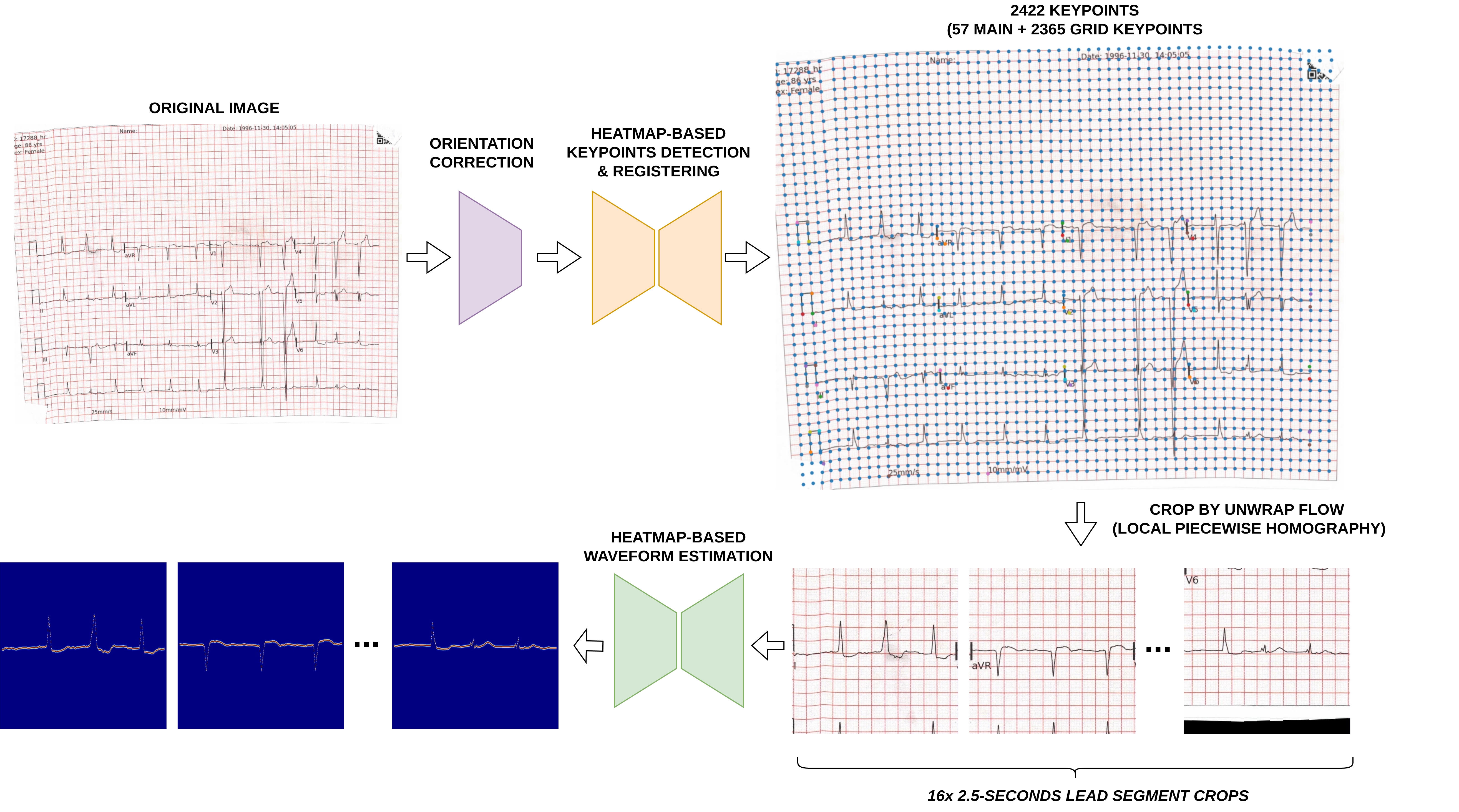\n\n\n\n## Heatmap-based keypoints estimation\nA 2D UNet model was trained to predict 57 \"feature-rich\" keypoints and `43*55=2365` grid keypoints, as shown in the figure below.\n\n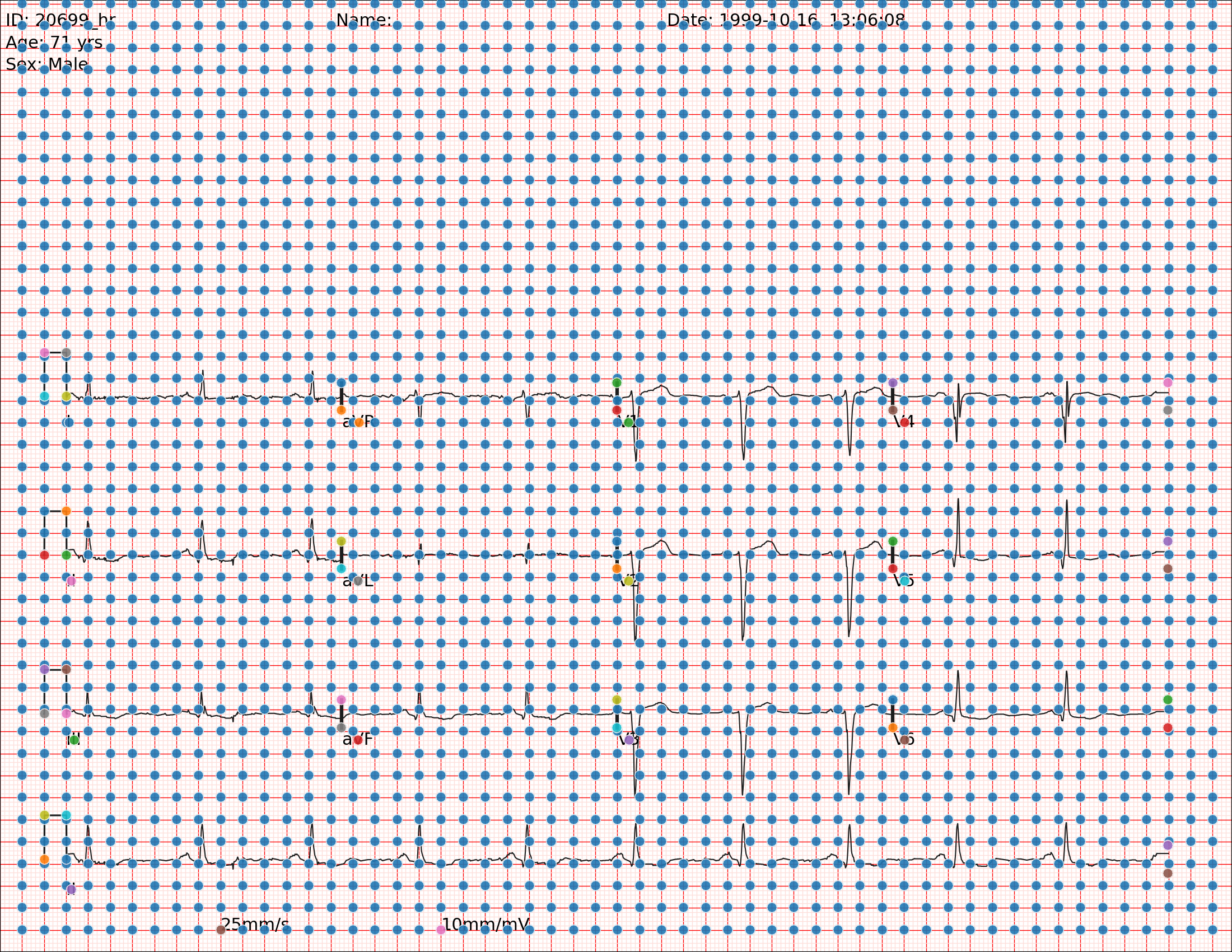\n\n\nI obtained the exact coordinates for all 2,422 keypoints by inspecting the [ecg-image-kit](https://github.com/alphanumericslab/ecg-image-kit) source code. The \"main\" keypoints were heuristically selected, typically around the calibration pulses, splitting ticks, and lead names, which I consider to have rich local features.\n\n> **Note:** I ignored some near-border grid keypoints since they could confuse the model. However, this caused many headaches in the subsequent registering stage. Perhaps keeping all `44*57` instead of just `42*55` keypoints would have been a better choice :D\n\n### Very good initial pseudo label\nI use one of the SOTA opensource dense matching model [MINIMA-RoMa](https://github.com/LSXI7/MINIMA) to obtain very accurate initial pseudo-labeled keypoints. This involved simply matching the type 0001 image to each image in the training set.\n\n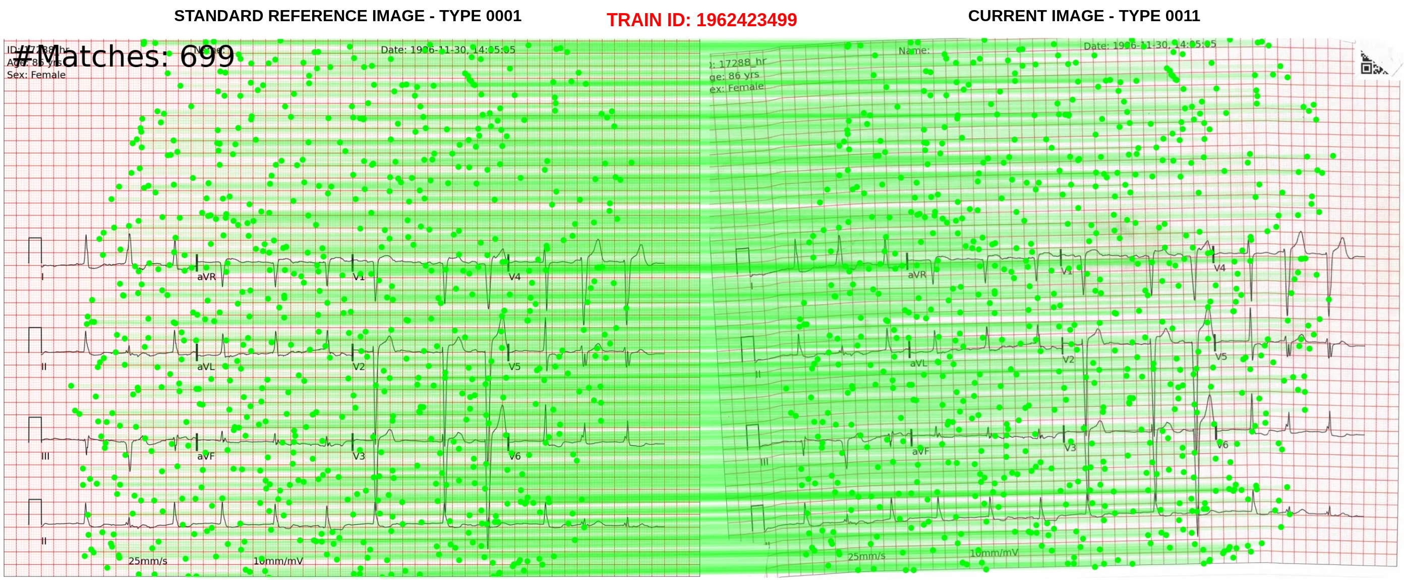\n\n\nNote that I did not perform matching followed by Homography matrix estimation to warp reference keypoints into current image's space, because it generates wrong keypoint coordinates if the scene is non-planar or if local distortion is heavy. Instead, for modern dense matching models (LoFTR, RoMA, etc.), we can resample/interpolate the predicted warping flow at arbitrary coordinates in an image to estimate the sub-pixel level matched keypoint coordinates on the remaining one.\n\nYou can try more recent SOTA methods on Image Matching very quickly using this awesome demo: https://huggingface.co/spaces/Realcat/image-matching-webui\n\n\n### Modeling\nA 2D UNet model was trained to predict a 58-channel output heatmap:\n- **First channel:** Single 2D heatmap encoding the spatial location of all 2,365 grid keypoints. For each keypoint, a small unnormalized Gaussian-like heatmap centered on that keypoint is drawn, with `sigma=2 px` relative to the standard reference image (type 0001, `1700x2200`), adaptively scaled based on the current image's scale (relative to the reference).\n- **Last 57 channels:** Each channel encodes the location of a single \"main/feature-rich\" keypoint, also using a Gaussian heatmap with `sigma=2px`, similar to the setting above.\n\n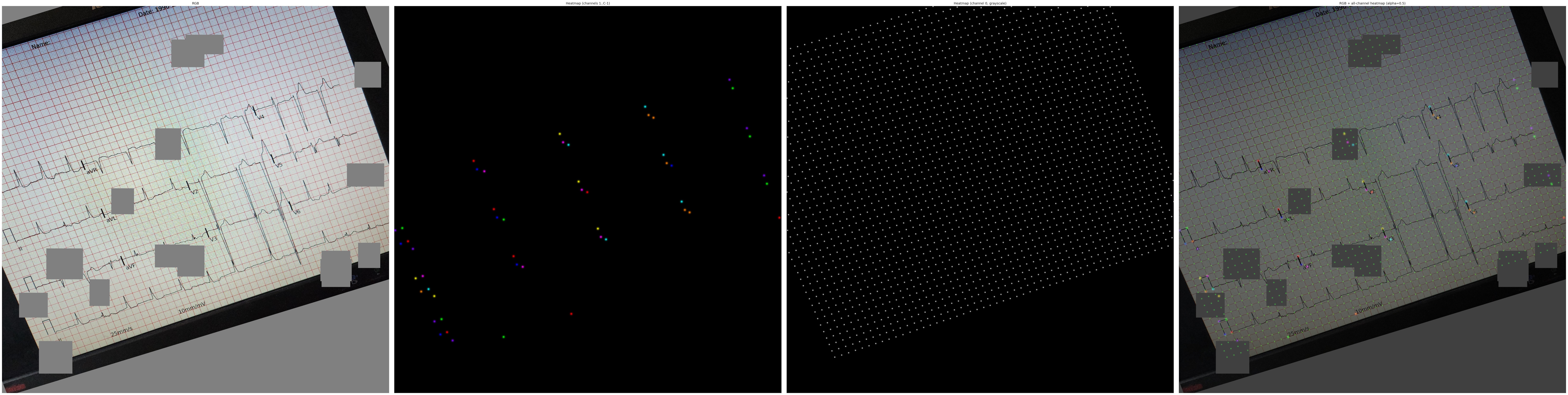\n*Visualization of an augmented train samples, left to right: augmented image, visualization of 2nd-58th heatmap channels, first channel encode grid points, overlayed visualization*\n\n\nThe model was trained end-to-end using multi-task losses. Despite the fact that the network can be trained using just BCE loss, I used BCE for the first channel and Channel-Masked JSD (Jensen-Shannon Divergence) for the remaining 57 channels. Each of the 57 channels encodes only a single keypoint Gaussian heatmap; the spatial distribution has 0 peaks (when the keypoint is outside the image) or 1 peak (unimodal), unlike the multiple peaks (multimodal) distribution of the first channel. Thus, a spatial distribution-based loss (JSD, KLDiv, CE) provides better inductive bias/regularization compared to BCE. Using JSD allows for much faster convergence, which I have confirmed in almost every experiment/project I have finished in the past.\n\nAdditionally, scaling the image size proved better than scaling the model size. We already know that the pattern/context is not very hard to predict for a model in this particular task (I found MaxVit, a hybrid CNN-Transformer, did not outperform a ConvNeXT-small with a much more limited receptive field). Therefore, local pattern recognition is sufficient, allowing the use of a CNN-only architecture which is much easier to scale to larger image sizes. Larger image size is critically important to obtain a fine-grained heatmap with less sub-pixel error. Furthermore, if the ROI in the test image is much smaller than the captured image (e.g., the camera is far from the object), a `longest resize + padding` transform will destroy details, so resolution must be prioritized.\n\nI measured a keypoint metric similar to `AP@0.5-0.95` for grid keypoints and `Accuracy@0.5-0.95` for the 57 main keypoints to track the best model. The final config used to train the 5-fold models was:\n- `3x2048x2048` image size, longest resize + padding with bicubic interpolation.\n- Output heatmap has a stride of 1, shape of `58x2048x2048`.\n- **Model:**\n - Encoder: ConvNeXT-small ([convnext_small.fb_in22k_ft_in1k_384](https://huggingface.co/timm/convnext_small.fb_in22k_ft_in1k_384))\n - Decoder: Standard SMP UNet Decoder with 4 blocks of `[384, 256, 128, 64]` channels. *Tried other options such as PixelShuffle-based decoder, but they did not outperform the baseline.*\n - MLP segmentation head: `64 -> 128 -> 58` with GELU and LayerNorm.\n- Heatmap Gaussian sigma is 2 pixels (*tuned*).\n- **Multi-task Losses (2 losses):** BCE (1st channel) + JSD (2nd-58th channels).\n- **Multi-task weighting:** GLS ([Geometric Loss Strategy](https://arxiv.org/pdf/1904.08492)). *GLS is good—not always the best—but almost the first one I will try in a MTL setup :D*\n- **Heavy Data Augmentation:** **Affine**, **Perspective**, **RandomCrop**, GrayScale, **RandomBrightnessContrast**, ColorJitter, Downscale, Blur, Noise, **Dropout (Coarse, Grid, XYMasking)** carefully designed to preserve enough information. RandomCrop and Dropout at the image level might help resolve occlusion/partial crops and encourage better global context learning.\n- AdamW optimizer with learning rate `1e-4`, Cosine scheduler.\n- Model EMA with decay=0.999.\n\nAfter the heatmap model was trained, I finetuned each fold model using an additional loss to achieve sub-pixel accuracy on main keypoint predictions: MSELoss on [DSNT](https://arxiv.org/pdf/1801.07372) prediction and groundtruth coordinates of shape `(57, 2)`, resulting in 3 total losses.\n\n\n### Iterative pseudo labeling\nI train 5 models on 5 folds to obtain the OOF predictions, decode, then some postprocessing logics defined in the subsequent section [Keypoint Registration](#keypoint-registration) was applied. This process is treated as a denoising process, where I hope model will learn the average/correct truth and skipping the small amount of noises in the initial pseudo label by MINIMA-RoMa. After 1 round, prediction is good enough and this round 1 pseudo label was used to train final keypoint estimation models for submission.\n\n\n## Keypoint Registration\nAfter obtaining the heatmap from the previous stage, the next task is to decode the heatmap into discrete keypoints and register/order them correctly. The following logic was applied sequentially:\n- **Decode the 57 main keypoints:** Simply `argmax` over the 2D spatial heatmap for each of the 2nd-58th output channels. This way, we already know the correct keypoint order. *We can use a confidence score to determine if a keypoint is outside the image region, but it's not trustworthy since the model is not supervised on \"out-of-region\" keypoints (channel-masked in JSD loss). Fortunately, subsequent stages are robust enough to handle WRONG predictions of outside-image keypoints.*\n- For the 5-fold models, we got `(5, 57, 2)` decoded main keypoints. Simply flatten to `(285, 2)`, using those \"nearly duplicated\" keypoints to estimate the Homography Transformation matrix H (strong assumption that it's an Affine transform) and the relative scale from the **standard reference image (type 0001)** to the current images. RANSAC is robust to outliers, so wrong predictions/noise from the previous stage are filtered.\n- NMS threshold (L2 distance) is set to 20 pixels in the reference image, adaptively scaled using the estimated relative scale mentioned above to be suitable for the current image -> decode the first channel \"grid\" heatmap into a list (variable length) of grid keypoints.\n- Now the only remaining task is a 1:1 mapping between the list of predicted grid keypoints and the 2365 reference grid keypoints. It seems easy at first glance, but there are many edge cases that happen in real life (and possibly in the private test set). A multi-stage matching algorithm was developed which solved all provided cases in the training set, though I pretty sure it's not perfect. It would be long to describe fully, but here are some key ideas behind it:\n - Using the Homography transformation matrix H estimated in the previous step, we have a bijection between the current coordinate space and the reference coordinate space.\n - Linear Assignment Matching (Hungarian algorithm) using pairwise L2 distance as the cost matrix, disabling \"impossible\" matching via a proper gating cost.\n - Use a strict threshold, e.g., 8 pixels error allowed. This prevents False Positive matches where a predicted keypoint is wrongly matched to a reference keypoint. If the paper is not planar but curved/creased/wrinkled, then H is no longer accurate, so only a fraction of predicted keypoints will be matched.\n - Based on high-confidence matched keypoints, recompute/interpolate nearby reference keypoints using a local Homography matrix (estimated from nearby matches only) computed for **each** keypoint.\n - This happens in a loop until no new matches are found, iteratively matching all predicted keypoints and registering them with correct indices. Missed detections will be replaced by an accurate interpolated version using information from just the nearby predicted keypoints, partially solving the \"local distortion\" problem.\n- In the end, for each image, we obtain an accurate list of 2,422 keypoints (2365 grid keypoints + 57 main keypoints).\n\n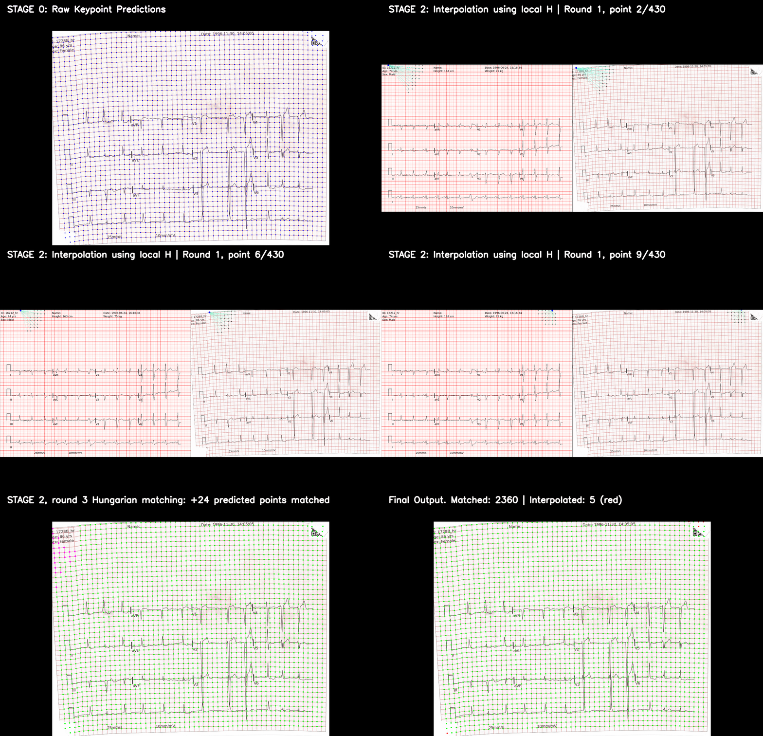\n*This GIF describes how the keypoints registering algorithm worked step by step*\n\n\n## Lead Cropping\n\nGiven the original images and 2,422 keypoints estimated from the previous stage, we can proceed to cropping. All images use the same reference template (type 0001), so it's easier to crop out an arbitrary region of interest, predefined using coordinates in the reference template. Several cropping methods were tested:\n1. Estimate a single Homography matrix mapping from the current image to the reference image using nearby \"main\" keypoints.\n2. Estimate a Piecewise Homography matrix mapping each cell (defined by 4 grid corners) from the current image to the reference image, using `cv.getPerspectiveTransform` locally -> compute flow map -> resample using `cv2.remap` (or `F.grid_sample` or `scipy.ndimage.map_coordinates`).\n3. Same idea as (2), but using `scipy.interpolate.RectBivariateSpline`.\n4. Same as (2), but for each cell, using `cv2.findHomography` to find a local Homography on **K=16** nearby keypoints instead of just **K=4** as in (2).\n\n\n\nMethod (4) performed the best, since it is not too global as in (1) but keeps the \"locality\" property enough to well-handle local distortion, without being too strictly local and sensitive to grid keypoint estimation errors as in (2).\n\n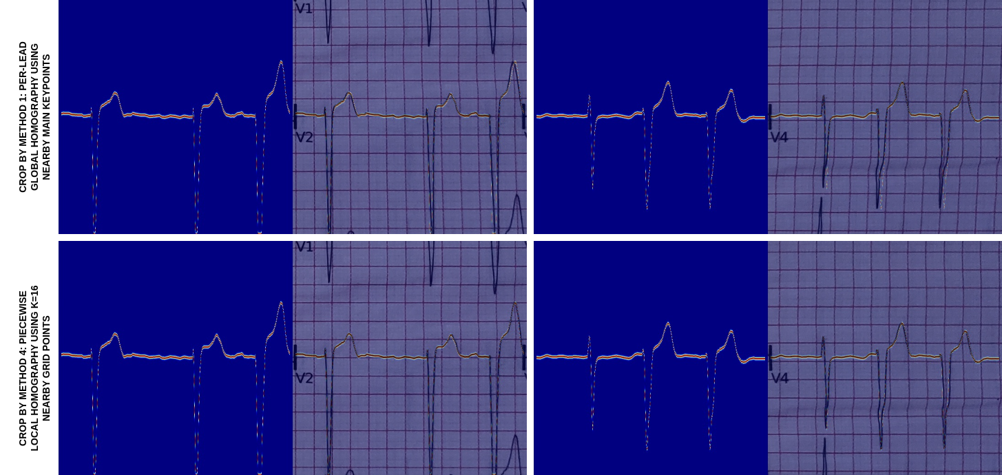\n*Misalignment due to local distortion using method (1) - see the sharp peaks, but much better results were obtained using method (4)*\n\n\n## Heatmap-based lead waveform estimation\n\nGiven a warped crop of each lead, another UNet was trained to predict a 2D heatmap of the lead waveform.\nI think the encoding scheme (codec) is important here. For each lead, I crop out the lead image region slightly wider on both the left and right to prevent slight rectification errors from the previous stage destroying the signal needed for prediction. That is, even if the crop is left-shifted or right-shifted by a small number of pixels, the rendered waveform is still fully included in the image, thus can be recovered by a good model.\n\n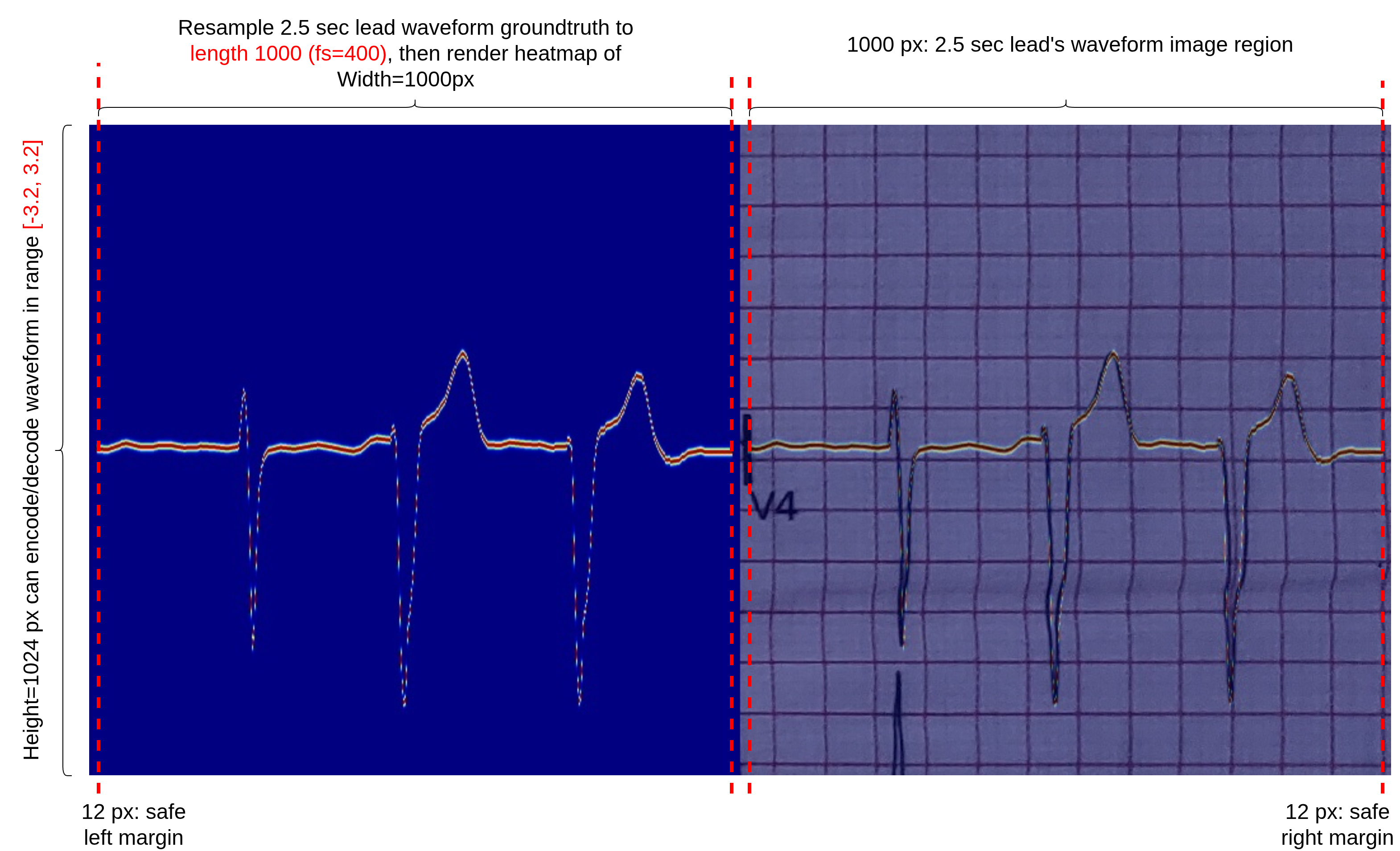\n\n\nAs for the heatmap, I render it in a column-independent way. Each column is an unnormalized 1D-Gaussian heatmap with 1 peak (mu) at the groundtruth value, and a std (sigma) value is fixed or adaptively changed based on the waveform itself. So, each column always represents a probability distribution with a single peak. This codec scheme is \"nearly lossless\", i.e., it maintains a very high SNR during the encoding and decoding back (recomputing expectation from a probability density function) operation.\n\n### Modeling\n\n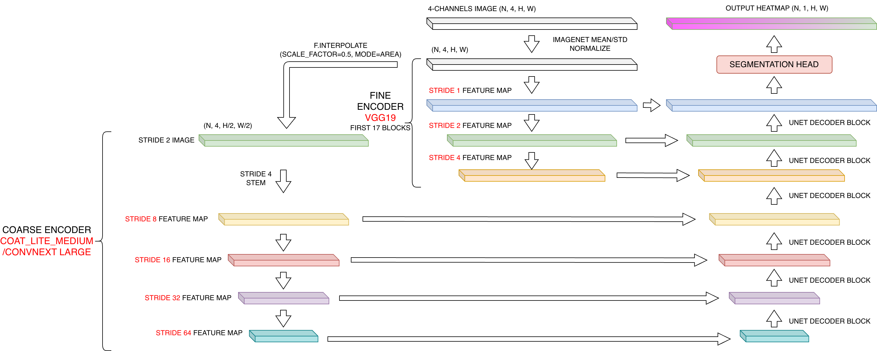\n*UNet architecture with dual-encoder. A VGG19 encodes finegrained features at stride 1/2/4 while another coarse encoder of either CoaT Lite Medium or ConvNeXT Large aggregate global/nearby information, better handles occlusion or captures long-range dependencies*\n\n\nIndeed, I had not trained this final architecture before; I just trained it once on all data to get a single checkpoint to submitted just before by the deadline. The hyperparameters were selected based on heuristics and previous experiments, in which I combined everything \"that should work\" into the final trial. All previous experiments did not introduce the VGG19 fine-grained/high-resolution encoder, but rather relied on a simpler baseline:\n- Image size `512x512`, GT waveform is resampled to a fixed length of 500, GT heatmap has shape `(1, 512, 512)` where the center region `(1, 512, 500)` actually encodes the GT waveform.\n- Rectification using method (2), Piecewise Perspective Transform (`K=4`).\n- UNet model with ConvNext-small encoder, a standard SMP UNet decoder which outputs a heatmap of **stride 1**, shape `(1, 512, 512)`.\n- Column-wise JSD Loss (i.e., `F.softmax(dim=2)` on predicted tensor of shape `NCHW`).\n\n**Some key insights:**\n- Warping **interpolation mode** matters to prevent losing very fine-grained details: `cv2.INTER_LANCZOS4` performed the best and was used in almost all experiments.\n- Heatmap Gaussian sigma is 2px relative to the reference template image 0001.\n- Adaptive sigma scale: The rationale behind this is that some parts of the waveform are harder to predict than others, e.g., sharp peaks where the magnitude significantly changes in a short time, resulting in a \"near straight line\" parallel to the mV axis. A simple method was applied which increases the sigma value for waveform values where the local standard deviation is large. Its effectiveness was validated by an improvement in local CV.\n ```python\n SIGMA, ADAPTIVE_FACTOR = 2, 0.4\n local_abs_diff = 0.5 * (np.abs(arr - np.r_[arr[0], arr[:-1]]) + np.abs(arr - np.r_[arr[1:], arr[-1]]))\n # 3-sigma rule: if > 3*sigma, start using scale >= 1\n adaptive_sigma_arr = SIGMA + ADAPTIVE_FACTOR * np.maximum(local_abs_diff - 3 * SIGMA, 0) / 3\n ```\n\n 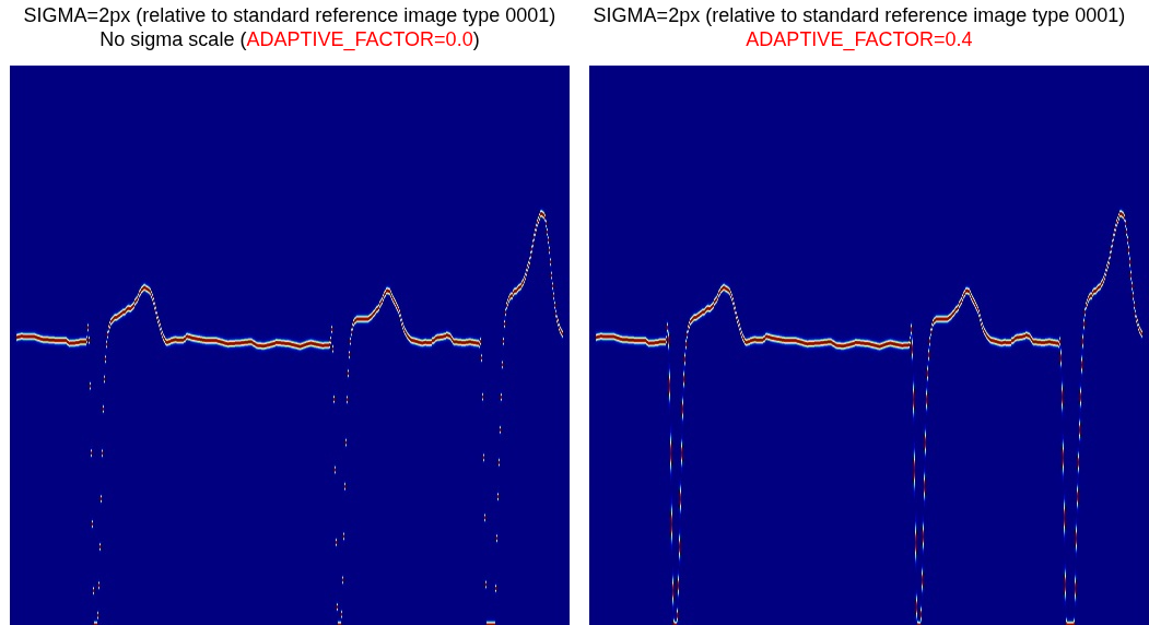\n\n\n* Column-wise JSD loss was used. *In short: `JSD` > `CE` >> `BCE`.*\n* UNet Decoder: The final model uses 6 UNet Decoder blocks, decoder channels `[256,192,160,128,96,64]` corresponding to stride `64 -> 1` with LayerNorm and GELU activation. *Performance scales better with the number of parameters. A higher number of channels in the high-resolution feature map is needed to preserve fine-grained texture details, but this also increases memory heavily. For the upscale type, a PixelShuffle-based Decoder was tried but didn't outperform the traditional F.interpolate(). Deformable Convolution (v2 or v4) was also tried as a drop-in replacement for traditional nn.Conv2d and showed better performance, but was not used due to slower runtime; I argued that gains came from the increased parameter count instead.*\n* Resolution matters: The use of an **input image size of 1024** is critical to keep texture details, bringing significant gains over 512. *Before this, I tested if the gain came from higher input resolution or higher output resolution by sweeping over some modeling configs:*\n * *Image size 512, output heatmap size 1024 (stride 0.5 with an additional x2 upscale UNet Decoder block)*\n * *Image size 512, change encoder stride from 4 to 1 or 2 (modifying the first stem convolution stride)*\n * *Image size 1024, output heatmap size 512*\n * *(Much better) Image size 1024, output heatmap size 1024*\n\n\n* Main encoder: CoAT and ConvNext-large were used. The two architectures show different characteristics. CoAT tends to be slightly better on noisy and occluded image types, possibly due to a larger receptive field and more input-dynamic nature, hence it can use nearby information to guess what is under occlusion. Meanwhile, ConvNext is better at locality and extracting fine-grained features, hence better SNR on good and high-resolution images such as phone photos.\n\n 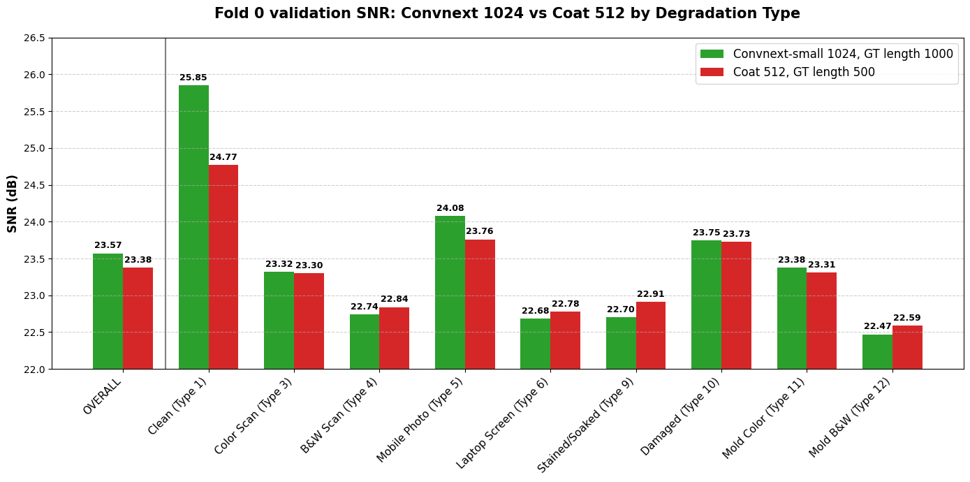\n \n *Comparison is unfair due to different image sizes (1024 vs 512), but still shows some characteristics of each architecture: pure-CNN vs Hybrid CNN-Transformer.*\n\n* **The \"fine\" encoder**: VGG19 encoder to extract feature maps at stride 1/2/4. We know that this task strongly benefits from low-level feature maps and high resolution, and VGG is one of the very few architectures which outputs a stride 1 feature map by default. VGG is also used in [RoMA](https://arxiv.org/abs/2305.15404) and proved to be better than ResNet-like architectures in extracting fine-grained local features. I used [vgg19.tv_in1k](https://huggingface.co/timm/vgg19.tv_in1k) which does not use BatchNorm, inspired by Image Super Resolution literature ([EDSR](https://arxiv.org/abs/1707.02921))\n* **The blank template**: I use [ecg-image-kit](https://github.com/alphanumericslab/ecg-image-kit) to render an empty image without any lead waveform, acting as a blank template with just grids, calibration pulses, separation ticks, and lead names. Each lead crop was concatenated with the corresponding grayscale blank template, resulting in a 4-channel image to be passed to the 2D UNet model, instead of the original 3-channel RGB image. I hypothesize the template is useful for the model to better learn the local correlation between the rectified image and the standard grid template (aligned perfectly with groundtruth heatmap), allowing it to internally learn to alignment accordingly. It also reduces the complexity of learning lead-specific grid layouts, hence faster convergence\n\n 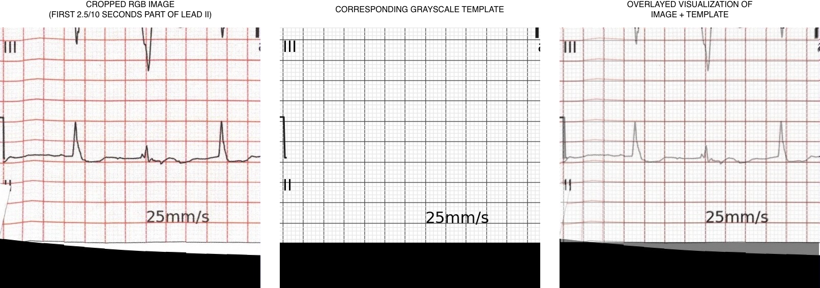\n\n* Augmentation: The key augmentation was to add a small amount of noise (following a truncated normal distribution with `sigma=0.4px`) into the detected grid keypoints before the lead cropping procedure (using local Piecewise Homography transform (2)). This mimics real-life errors since the keypoint detector's prediction is not perfectly accurate. I found not much gain from usual augmentations like ColorJitter, BrightnessContrast, Grayscale, or very small Affine/Perspective transforms, so I set these augmentation probabilities to a small value p=0.1\n* Training: AdamW optimizer, Cosine LR scheduler, gradient clipping by norm of 1.0, and models are trained for about 70K steps with an effective batch size of 8 (batch size 2, gradient accumulation 4)\n* Model EMA with decay=0.999\n\n\n### ABLATION STUDY\nDetails in [the training code repo](https://github.com/dangnh0611/kaggle_ecg_digitization/blob/main/docs/ABLATION_STUDY.md)\n\n## Image orientation correction\nThere are 69 rotated image in the training set. Not sure how many in test set, and wrong orientation will affect the keypoints detection stage. So I train a simple model to correct/standardize image orientation.\n\nFor each image, we can get the exact rotation angle relative to the standard reference image using Homography H. I simply trained a [efficientvit_b2.r224_in1k](https://huggingface.co/timm/efficientvit_b2.r224_in1k) to jointly predict one of 4 possible rotations 0/90/180/270 degrees (classification task) and the exact rotation angle encoded by sine/cosine (regression task). During training, heavy augmentation was applied to ensure the trained model would be robust on the unseen private test set. Of course, the training task is just too easy, so the validation accuracy is 100% and angle MAE is just around 1.1 degrees.\n\n\n## Final submission\n\nI wrote the inference code and submitted it near the deadline; everything was a mess and aweful on that last day..\nAll submissions include the inference pipeline for a single Image Rotation/Orientation model and 5-fold keypoint detection models.\n\nThe first 4 submissions all estimate lead waveforms using a single model without ensemble, and prediction dynamic was also limited to the range `[-3.2, 3.2]` due to the nature of the heatmap codec. Interestingly, just scaling the image size did not work—my model did not generalize well to the new input size. That is, training on input size `[512, 512]` (which can encode `[-3.2, 3.2]` waveforms) and then inferencing on input size `[1024, 512]` (which can encode `[-6.4, 6.4]` waveforms) resulted in very bad SNR.\n\n4 single models were submitted:\n\n* (1) Dual Encoder CoaT Lite Medium + VGG19 on image size `[1024, 1024]`, output heatmap of size `[1024, 1024]` (*first time training, no validation*).\n* (2) Dual Encoder ConvNeXT Large + VGG19 on image size `[1024, 1024]`, output heatmap of size `[1024, 1024]` (*first time training, no validation*).\n* (3) Single Encoder CoaT Lite Medium on image size `[512, 512]`, output heatmap of size `[512, 512]` (*best learning rate is known*).\n* (4) Single Encoder ConvNeXT small on image size `[1024, 1024]`, output heatmap of size `[1024, 1024]` (*best learning rate is known*).\n\nThe final submission:\n\n* Ensemble of (1) and (2) with corresponding weights of 0.7-0.3.\n* Lead II first quarter of 2.5 seconds fusion with weights 0.5-0.5.\n* Luckily, a single \"TALL\" model (single encoder ConvNeXT-small) accepting an input size of `[1024, 512]` and able to handle waveforms in the range `[-6.4, 6.4]` was trained and finished in time, but just scored relatively low (`SNR~21.7` on single validation fold) due to limitted tunning and training steps. But it is enough, and was used to solve the limited range of the main models, acting as a refinement stage where the first stage's predictions were near the limitation, e.g., `np.abs(prediction_signal)` close to 3.2.\n* It successfully scored 22.93 on LB and 22.63 on PB, finished just 8 minutes before the competition deadline—that's insane..\n\n\n| **MODEL** | **SNR ON TRAIN SET** | **Public LB** | **Private LB** | |\n|:-------------------------------------------------------------------------------------------:|:--------------------:|:--------------:|:--------------:|---|\n| Dual Encoder CoaT Lite Medium + VGG19, image size 1024, heatmap size 1024 | **28.006985** | **22.63859** | **22.34824** | |\n| Dual Encoder ConvNeXT Large + VGG19, image size 1024, heatmap size 1024 | 27.484089 | 22.43810 | 22.15886 | |\n| Single Encoder CoaT Lite Medium, image size 512, heatmap size 512 | 26.050978 | 21.93992 | 21.80577 | |\n| Single Encoder ConvNeXT small, image size 1024, heatmap size 1024 | 26.081009 | 22.04173 | 21.78336 | |\n| Ensemble (1) and (2) with weight 0.7-0.3, lead fusion, refinement using TALL model 1024x512 | _N/A_ | **_22.93061_** | **_22.62929_** | |\n\n\n## Source code\n\n* **Training code**: https://github.com/dangnh0611/kaggle_ecg_digitization\n* **Inference notebook**: https://www.kaggle.com/code/dangnh0611/5th-place-solution\n\n\n---\nThanks for your attention!", "votes": null }, { "id": "3397370", "postDate": "01/27/2026 05:42:36", "content": "This solution is fantastic. I'm truly impressed!
", "rawMarkdown": "This solution is fantastic. I'm truly impressed!", "votes": null }, { "id": "3397900", "postDate": "01/28/2026 08:36:30", "content": "Congratulations @dangnh0611
", "rawMarkdown": "Congratulations @dangnh0611", "votes": null }, { "id": "3400817", "postDate": "02/02/2026 11:16:18", "content": "OMG, thanks for the detail solution and congrats on your prize anh @dangnh0611
", "rawMarkdown": "OMG, thanks for the detail solution and congrats on your prize anh @dangnh0611", "votes": null }, { "id": "3401054", "postDate": "02/02/2026 20:42:47", "content": "A cảm ơn nhiều 😄
", "rawMarkdown": "A cảm ơn nhiều 😄", "votes": null } ], "comments": [ { "id": 3397370, "author_name": "cudacoding", "author_url": "", "post_date": "01/27/2026 05:42:36", "content": "This solution is fantastic. I'm truly impressed!
", "votes": null, "replies": [] }, { "id": 3397900, "author_name": "navneetbende", "author_url": "", "post_date": "01/28/2026 08:36:30", "content": "Congratulations @dangnh0611
", "votes": null, "replies": [] }, { "id": 3400817, "author_name": "locbaop", "author_url": "", "post_date": "02/02/2026 11:16:18", "content": "OMG, thanks for the detail solution and congrats on your prize anh @dangnh0611
", "votes": null, "replies": [ { "id": 3401054, "author_name": "dangnh0611", "author_url": "", "post_date": "02/02/2026 20:42:47", "content": "A cảm ơn nhiều 😄
", "votes": null, "replies": [] } ] } ], "raw_markdown_by_id": { "3397276": "Many thanks to the competition host and Kaggle for another engaging challenge—and congratulations to all the participants!\n\nAs always, I had a great time learning throughout the competition. It was indeed a crazy race to the deadline for me, filled with many emotions until the very end. I am really happy to share a few thoughts on my solution here.\n\n**Changelogs**:\n- 2025/02/06: update [some Ablation Study](https://github.com/dangnh0611/kaggle_ecg_digitization/blob/main/docs/ABLATION_STUDY.md)\n\n## The overall pipeline\n\n\n\n\n\n## Heatmap-based keypoints estimation\nA 2D UNet model was trained to predict 57 \"feature-rich\" keypoints and `43*55=2365` grid keypoints, as shown in the figure below.\n\n\n\n\nI obtained the exact coordinates for all 2,422 keypoints by inspecting the [ecg-image-kit](https://github.com/alphanumericslab/ecg-image-kit) source code. The \"main\" keypoints were heuristically selected, typically around the calibration pulses, splitting ticks, and lead names, which I consider to have rich local features.\n\n> **Note:** I ignored some near-border grid keypoints since they could confuse the model. However, this caused many headaches in the subsequent registering stage. Perhaps keeping all `44*57` instead of just `42*55` keypoints would have been a better choice :D\n\n### Very good initial pseudo label\nI use one of the SOTA opensource dense matching model [MINIMA-RoMa](https://github.com/LSXI7/MINIMA) to obtain very accurate initial pseudo-labeled keypoints. This involved simply matching the type 0001 image to each image in the training set.\n\n\n\n\nNote that I did not perform matching followed by Homography matrix estimation to warp reference keypoints into current image's space, because it generates wrong keypoint coordinates if the scene is non-planar or if local distortion is heavy. Instead, for modern dense matching models (LoFTR, RoMA, etc.), we can resample/interpolate the predicted warping flow at arbitrary coordinates in an image to estimate the sub-pixel level matched keypoint coordinates on the remaining one.\n\nYou can try more recent SOTA methods on Image Matching very quickly using this awesome demo: https://huggingface.co/spaces/Realcat/image-matching-webui\n\n\n### Modeling\nA 2D UNet model was trained to predict a 58-channel output heatmap:\n- **First channel:** Single 2D heatmap encoding the spatial location of all 2,365 grid keypoints. For each keypoint, a small unnormalized Gaussian-like heatmap centered on that keypoint is drawn, with `sigma=2 px` relative to the standard reference image (type 0001, `1700x2200`), adaptively scaled based on the current image's scale (relative to the reference).\n- **Last 57 channels:** Each channel encodes the location of a single \"main/feature-rich\" keypoint, also using a Gaussian heatmap with `sigma=2px`, similar to the setting above.\n\n\n*Visualization of an augmented train samples, left to right: augmented image, visualization of 2nd-58th heatmap channels, first channel encode grid points, overlayed visualization*\n\n\nThe model was trained end-to-end using multi-task losses. Despite the fact that the network can be trained using just BCE loss, I used BCE for the first channel and Channel-Masked JSD (Jensen-Shannon Divergence) for the remaining 57 channels. Each of the 57 channels encodes only a single keypoint Gaussian heatmap; the spatial distribution has 0 peaks (when the keypoint is outside the image) or 1 peak (unimodal), unlike the multiple peaks (multimodal) distribution of the first channel. Thus, a spatial distribution-based loss (JSD, KLDiv, CE) provides better inductive bias/regularization compared to BCE. Using JSD allows for much faster convergence, which I have confirmed in almost every experiment/project I have finished in the past.\n\nAdditionally, scaling the image size proved better than scaling the model size. We already know that the pattern/context is not very hard to predict for a model in this particular task (I found MaxVit, a hybrid CNN-Transformer, did not outperform a ConvNeXT-small with a much more limited receptive field). Therefore, local pattern recognition is sufficient, allowing the use of a CNN-only architecture which is much easier to scale to larger image sizes. Larger image size is critically important to obtain a fine-grained heatmap with less sub-pixel error. Furthermore, if the ROI in the test image is much smaller than the captured image (e.g., the camera is far from the object), a `longest resize + padding` transform will destroy details, so resolution must be prioritized.\n\nI measured a keypoint metric similar to `AP@0.5-0.95` for grid keypoints and `Accuracy@0.5-0.95` for the 57 main keypoints to track the best model. The final config used to train the 5-fold models was:\n- `3x2048x2048` image size, longest resize + padding with bicubic interpolation.\n- Output heatmap has a stride of 1, shape of `58x2048x2048`.\n- **Model:**\n - Encoder: ConvNeXT-small ([convnext_small.fb_in22k_ft_in1k_384](https://huggingface.co/timm/convnext_small.fb_in22k_ft_in1k_384))\n - Decoder: Standard SMP UNet Decoder with 4 blocks of `[384, 256, 128, 64]` channels. *Tried other options such as PixelShuffle-based decoder, but they did not outperform the baseline.*\n - MLP segmentation head: `64 -> 128 -> 58` with GELU and LayerNorm.\n- Heatmap Gaussian sigma is 2 pixels (*tuned*).\n- **Multi-task Losses (2 losses):** BCE (1st channel) + JSD (2nd-58th channels).\n- **Multi-task weighting:** GLS ([Geometric Loss Strategy](https://arxiv.org/pdf/1904.08492)). *GLS is good—not always the best—but almost the first one I will try in a MTL setup :D*\n- **Heavy Data Augmentation:** **Affine**, **Perspective**, **RandomCrop**, GrayScale, **RandomBrightnessContrast**, ColorJitter, Downscale, Blur, Noise, **Dropout (Coarse, Grid, XYMasking)** carefully designed to preserve enough information. RandomCrop and Dropout at the image level might help resolve occlusion/partial crops and encourage better global context learning.\n- AdamW optimizer with learning rate `1e-4`, Cosine scheduler.\n- Model EMA with decay=0.999.\n\nAfter the heatmap model was trained, I finetuned each fold model using an additional loss to achieve sub-pixel accuracy on main keypoint predictions: MSELoss on [DSNT](https://arxiv.org/pdf/1801.07372) prediction and groundtruth coordinates of shape `(57, 2)`, resulting in 3 total losses.\n\n\n### Iterative pseudo labeling\nI train 5 models on 5 folds to obtain the OOF predictions, decode, then some postprocessing logics defined in the subsequent section [Keypoint Registration](#keypoint-registration) was applied. This process is treated as a denoising process, where I hope model will learn the average/correct truth and skipping the small amount of noises in the initial pseudo label by MINIMA-RoMa. After 1 round, prediction is good enough and this round 1 pseudo label was used to train final keypoint estimation models for submission.\n\n\n## Keypoint Registration\nAfter obtaining the heatmap from the previous stage, the next task is to decode the heatmap into discrete keypoints and register/order them correctly. The following logic was applied sequentially:\n- **Decode the 57 main keypoints:** Simply `argmax` over the 2D spatial heatmap for each of the 2nd-58th output channels. This way, we already know the correct keypoint order. *We can use a confidence score to determine if a keypoint is outside the image region, but it's not trustworthy since the model is not supervised on \"out-of-region\" keypoints (channel-masked in JSD loss). Fortunately, subsequent stages are robust enough to handle WRONG predictions of outside-image keypoints.*\n- For the 5-fold models, we got `(5, 57, 2)` decoded main keypoints. Simply flatten to `(285, 2)`, using those \"nearly duplicated\" keypoints to estimate the Homography Transformation matrix H (strong assumption that it's an Affine transform) and the relative scale from the **standard reference image (type 0001)** to the current images. RANSAC is robust to outliers, so wrong predictions/noise from the previous stage are filtered.\n- NMS threshold (L2 distance) is set to 20 pixels in the reference image, adaptively scaled using the estimated relative scale mentioned above to be suitable for the current image -> decode the first channel \"grid\" heatmap into a list (variable length) of grid keypoints.\n- Now the only remaining task is a 1:1 mapping between the list of predicted grid keypoints and the 2365 reference grid keypoints. It seems easy at first glance, but there are many edge cases that happen in real life (and possibly in the private test set). A multi-stage matching algorithm was developed which solved all provided cases in the training set, though I pretty sure it's not perfect. It would be long to describe fully, but here are some key ideas behind it:\n - Using the Homography transformation matrix H estimated in the previous step, we have a bijection between the current coordinate space and the reference coordinate space.\n - Linear Assignment Matching (Hungarian algorithm) using pairwise L2 distance as the cost matrix, disabling \"impossible\" matching via a proper gating cost.\n - Use a strict threshold, e.g., 8 pixels error allowed. This prevents False Positive matches where a predicted keypoint is wrongly matched to a reference keypoint. If the paper is not planar but curved/creased/wrinkled, then H is no longer accurate, so only a fraction of predicted keypoints will be matched.\n - Based on high-confidence matched keypoints, recompute/interpolate nearby reference keypoints using a local Homography matrix (estimated from nearby matches only) computed for **each** keypoint.\n - This happens in a loop until no new matches are found, iteratively matching all predicted keypoints and registering them with correct indices. Missed detections will be replaced by an accurate interpolated version using information from just the nearby predicted keypoints, partially solving the \"local distortion\" problem.\n- In the end, for each image, we obtain an accurate list of 2,422 keypoints (2365 grid keypoints + 57 main keypoints).\n\n\n*This GIF describes how the keypoints registering algorithm worked step by step*\n\n\n## Lead Cropping\n\nGiven the original images and 2,422 keypoints estimated from the previous stage, we can proceed to cropping. All images use the same reference template (type 0001), so it's easier to crop out an arbitrary region of interest, predefined using coordinates in the reference template. Several cropping methods were tested:\n1. Estimate a single Homography matrix mapping from the current image to the reference image using nearby \"main\" keypoints.\n2. Estimate a Piecewise Homography matrix mapping each cell (defined by 4 grid corners) from the current image to the reference image, using `cv.getPerspectiveTransform` locally -> compute flow map -> resample using `cv2.remap` (or `F.grid_sample` or `scipy.ndimage.map_coordinates`).\n3. Same idea as (2), but using `scipy.interpolate.RectBivariateSpline`.\n4. Same as (2), but for each cell, using `cv2.findHomography` to find a local Homography on **K=16** nearby keypoints instead of just **K=4** as in (2).\n\n\n\nMethod (4) performed the best, since it is not too global as in (1) but keeps the \"locality\" property enough to well-handle local distortion, without being too strictly local and sensitive to grid keypoint estimation errors as in (2).\n\n\n*Misalignment due to local distortion using method (1) - see the sharp peaks, but much better results were obtained using method (4)*\n\n\n## Heatmap-based lead waveform estimation\n\nGiven a warped crop of each lead, another UNet was trained to predict a 2D heatmap of the lead waveform.\nI think the encoding scheme (codec) is important here. For each lead, I crop out the lead image region slightly wider on both the left and right to prevent slight rectification errors from the previous stage destroying the signal needed for prediction. That is, even if the crop is left-shifted or right-shifted by a small number of pixels, the rendered waveform is still fully included in the image, thus can be recovered by a good model.\n\n\n\n\nAs for the heatmap, I render it in a column-independent way. Each column is an unnormalized 1D-Gaussian heatmap with 1 peak (mu) at the groundtruth value, and a std (sigma) value is fixed or adaptively changed based on the waveform itself. So, each column always represents a probability distribution with a single peak. This codec scheme is \"nearly lossless\", i.e., it maintains a very high SNR during the encoding and decoding back (recomputing expectation from a probability density function) operation.\n\n### Modeling\n\n\n*UNet architecture with dual-encoder. A VGG19 encodes finegrained features at stride 1/2/4 while another coarse encoder of either CoaT Lite Medium or ConvNeXT Large aggregate global/nearby information, better handles occlusion or captures long-range dependencies*\n\n\nIndeed, I had not trained this final architecture before; I just trained it once on all data to get a single checkpoint to submitted just before by the deadline. The hyperparameters were selected based on heuristics and previous experiments, in which I combined everything \"that should work\" into the final trial. All previous experiments did not introduce the VGG19 fine-grained/high-resolution encoder, but rather relied on a simpler baseline:\n- Image size `512x512`, GT waveform is resampled to a fixed length of 500, GT heatmap has shape `(1, 512, 512)` where the center region `(1, 512, 500)` actually encodes the GT waveform.\n- Rectification using method (2), Piecewise Perspective Transform (`K=4`).\n- UNet model with ConvNext-small encoder, a standard SMP UNet decoder which outputs a heatmap of **stride 1**, shape `(1, 512, 512)`.\n- Column-wise JSD Loss (i.e., `F.softmax(dim=2)` on predicted tensor of shape `NCHW`).\n\n**Some key insights:**\n- Warping **interpolation mode** matters to prevent losing very fine-grained details: `cv2.INTER_LANCZOS4` performed the best and was used in almost all experiments.\n- Heatmap Gaussian sigma is 2px relative to the reference template image 0001.\n- Adaptive sigma scale: The rationale behind this is that some parts of the waveform are harder to predict than others, e.g., sharp peaks where the magnitude significantly changes in a short time, resulting in a \"near straight line\" parallel to the mV axis. A simple method was applied which increases the sigma value for waveform values where the local standard deviation is large. Its effectiveness was validated by an improvement in local CV.\n ```python\n SIGMA, ADAPTIVE_FACTOR = 2, 0.4\n local_abs_diff = 0.5 * (np.abs(arr - np.r_[arr[0], arr[:-1]]) + np.abs(arr - np.r_[arr[1:], arr[-1]]))\n # 3-sigma rule: if > 3*sigma, start using scale >= 1\n adaptive_sigma_arr = SIGMA + ADAPTIVE_FACTOR * np.maximum(local_abs_diff - 3 * SIGMA, 0) / 3\n ```\n\n \n\n\n* Column-wise JSD loss was used. *In short: `JSD` > `CE` >> `BCE`.*\n* UNet Decoder: The final model uses 6 UNet Decoder blocks, decoder channels `[256,192,160,128,96,64]` corresponding to stride `64 -> 1` with LayerNorm and GELU activation. *Performance scales better with the number of parameters. A higher number of channels in the high-resolution feature map is needed to preserve fine-grained texture details, but this also increases memory heavily. For the upscale type, a PixelShuffle-based Decoder was tried but didn't outperform the traditional F.interpolate(). Deformable Convolution (v2 or v4) was also tried as a drop-in replacement for traditional nn.Conv2d and showed better performance, but was not used due to slower runtime; I argued that gains came from the increased parameter count instead.*\n* Resolution matters: The use of an **input image size of 1024** is critical to keep texture details, bringing significant gains over 512. *Before this, I tested if the gain came from higher input resolution or higher output resolution by sweeping over some modeling configs:*\n * *Image size 512, output heatmap size 1024 (stride 0.5 with an additional x2 upscale UNet Decoder block)*\n * *Image size 512, change encoder stride from 4 to 1 or 2 (modifying the first stem convolution stride)*\n * *Image size 1024, output heatmap size 512*\n * *(Much better) Image size 1024, output heatmap size 1024*\n\n\n* Main encoder: CoAT and ConvNext-large were used. The two architectures show different characteristics. CoAT tends to be slightly better on noisy and occluded image types, possibly due to a larger receptive field and more input-dynamic nature, hence it can use nearby information to guess what is under occlusion. Meanwhile, ConvNext is better at locality and extracting fine-grained features, hence better SNR on good and high-resolution images such as phone photos.\n\n \n \n *Comparison is unfair due to different image sizes (1024 vs 512), but still shows some characteristics of each architecture: pure-CNN vs Hybrid CNN-Transformer.*\n\n* **The \"fine\" encoder**: VGG19 encoder to extract feature maps at stride 1/2/4. We know that this task strongly benefits from low-level feature maps and high resolution, and VGG is one of the very few architectures which outputs a stride 1 feature map by default. VGG is also used in [RoMA](https://arxiv.org/abs/2305.15404) and proved to be better than ResNet-like architectures in extracting fine-grained local features. I used [vgg19.tv_in1k](https://huggingface.co/timm/vgg19.tv_in1k) which does not use BatchNorm, inspired by Image Super Resolution literature ([EDSR](https://arxiv.org/abs/1707.02921))\n* **The blank template**: I use [ecg-image-kit](https://github.com/alphanumericslab/ecg-image-kit) to render an empty image without any lead waveform, acting as a blank template with just grids, calibration pulses, separation ticks, and lead names. Each lead crop was concatenated with the corresponding grayscale blank template, resulting in a 4-channel image to be passed to the 2D UNet model, instead of the original 3-channel RGB image. I hypothesize the template is useful for the model to better learn the local correlation between the rectified image and the standard grid template (aligned perfectly with groundtruth heatmap), allowing it to internally learn to alignment accordingly. It also reduces the complexity of learning lead-specific grid layouts, hence faster convergence\n\n \n\n* Augmentation: The key augmentation was to add a small amount of noise (following a truncated normal distribution with `sigma=0.4px`) into the detected grid keypoints before the lead cropping procedure (using local Piecewise Homography transform (2)). This mimics real-life errors since the keypoint detector's prediction is not perfectly accurate. I found not much gain from usual augmentations like ColorJitter, BrightnessContrast, Grayscale, or very small Affine/Perspective transforms, so I set these augmentation probabilities to a small value p=0.1\n* Training: AdamW optimizer, Cosine LR scheduler, gradient clipping by norm of 1.0, and models are trained for about 70K steps with an effective batch size of 8 (batch size 2, gradient accumulation 4)\n* Model EMA with decay=0.999\n\n\n### ABLATION STUDY\nDetails in [the training code repo](https://github.com/dangnh0611/kaggle_ecg_digitization/blob/main/docs/ABLATION_STUDY.md)\n\n## Image orientation correction\nThere are 69 rotated image in the training set. Not sure how many in test set, and wrong orientation will affect the keypoints detection stage. So I train a simple model to correct/standardize image orientation.\n\nFor each image, we can get the exact rotation angle relative to the standard reference image using Homography H. I simply trained a [efficientvit_b2.r224_in1k](https://huggingface.co/timm/efficientvit_b2.r224_in1k) to jointly predict one of 4 possible rotations 0/90/180/270 degrees (classification task) and the exact rotation angle encoded by sine/cosine (regression task). During training, heavy augmentation was applied to ensure the trained model would be robust on the unseen private test set. Of course, the training task is just too easy, so the validation accuracy is 100% and angle MAE is just around 1.1 degrees.\n\n\n## Final submission\n\nI wrote the inference code and submitted it near the deadline; everything was a mess and aweful on that last day..\nAll submissions include the inference pipeline for a single Image Rotation/Orientation model and 5-fold keypoint detection models.\n\nThe first 4 submissions all estimate lead waveforms using a single model without ensemble, and prediction dynamic was also limited to the range `[-3.2, 3.2]` due to the nature of the heatmap codec. Interestingly, just scaling the image size did not work—my model did not generalize well to the new input size. That is, training on input size `[512, 512]` (which can encode `[-3.2, 3.2]` waveforms) and then inferencing on input size `[1024, 512]` (which can encode `[-6.4, 6.4]` waveforms) resulted in very bad SNR.\n\n4 single models were submitted:\n\n* (1) Dual Encoder CoaT Lite Medium + VGG19 on image size `[1024, 1024]`, output heatmap of size `[1024, 1024]` (*first time training, no validation*).\n* (2) Dual Encoder ConvNeXT Large + VGG19 on image size `[1024, 1024]`, output heatmap of size `[1024, 1024]` (*first time training, no validation*).\n* (3) Single Encoder CoaT Lite Medium on image size `[512, 512]`, output heatmap of size `[512, 512]` (*best learning rate is known*).\n* (4) Single Encoder ConvNeXT small on image size `[1024, 1024]`, output heatmap of size `[1024, 1024]` (*best learning rate is known*).\n\nThe final submission:\n\n* Ensemble of (1) and (2) with corresponding weights of 0.7-0.3.\n* Lead II first quarter of 2.5 seconds fusion with weights 0.5-0.5.\n* Luckily, a single \"TALL\" model (single encoder ConvNeXT-small) accepting an input size of `[1024, 512]` and able to handle waveforms in the range `[-6.4, 6.4]` was trained and finished in time, but just scored relatively low (`SNR~21.7` on single validation fold) due to limitted tunning and training steps. But it is enough, and was used to solve the limited range of the main models, acting as a refinement stage where the first stage's predictions were near the limitation, e.g., `np.abs(prediction_signal)` close to 3.2.\n* It successfully scored 22.93 on LB and 22.63 on PB, finished just 8 minutes before the competition deadline—that's insane..\n\n\n| **MODEL** | **SNR ON TRAIN SET** | **Public LB** | **Private LB** | |\n|:-------------------------------------------------------------------------------------------:|:--------------------:|:--------------:|:--------------:|---|\n| Dual Encoder CoaT Lite Medium + VGG19, image size 1024, heatmap size 1024 | **28.006985** | **22.63859** | **22.34824** | |\n| Dual Encoder ConvNeXT Large + VGG19, image size 1024, heatmap size 1024 | 27.484089 | 22.43810 | 22.15886 | |\n| Single Encoder CoaT Lite Medium, image size 512, heatmap size 512 | 26.050978 | 21.93992 | 21.80577 | |\n| Single Encoder ConvNeXT small, image size 1024, heatmap size 1024 | 26.081009 | 22.04173 | 21.78336 | |\n| Ensemble (1) and (2) with weight 0.7-0.3, lead fusion, refinement using TALL model 1024x512 | _N/A_ | **_22.93061_** | **_22.62929_** | |\n\n\n## Source code\n\n* **Training code**: https://github.com/dangnh0611/kaggle_ecg_digitization\n* **Inference notebook**: https://www.kaggle.com/code/dangnh0611/5th-place-solution\n\n\n---\nThanks for your attention!", "3397370": "This solution is fantastic. I'm truly impressed!", "3397900": "Congratulations @dangnh0611", "3400817": "OMG, thanks for the detail solution and congrats on your prize anh @dangnh0611", "3401054": "A cảm ơn nhiều 😄" }, "source": "meta" }