
First, I would like to thank the hosts and Kaggle for organizing this competition.\nI will explain my 4th place solution, focusing on the processing pipeline and model/training strategy.
\nMy approach focuses on rectification to make it easier for the model to recognize the signals, and then estimating the waveform using a regression model. Signal segmentation is treated only as an auxiliary task.
\nThe main points are:
\nThe process from input image to signal estimation is divided into 4 stages.
\n
For one high-resolution image, I use a sliding window (704x704 size, 0.5 overlap) to estimate the following using a multi-task model:
\n
Using the detected layout information, I estimate the image orientation and rotate it (0/90/180/270 degrees) to a unified upright orientation. The detected intersection coordinates are also rotated.
\nUsing the corrected image, the model estimates an index for each pixel indicating which vertical or horizontal line it belongs to.
\nThis determines where each intersection corresponds to in the grid (row, col).
I create a sampling coordinate field from the indexed intersections and warp the image to a fixed-size coordinate system. This method is the same as the grid_sample approach shared by @hengck23.\nThe output size is fixed at 1700x2200.
The rectified image often contains headers or margins, so I crop the top 25% to keep only the signal area.\nThen, I split the image width into 4 segments. The segment boundaries are determined by converting fixed column indices to pixels in the rectified image.
\nEach segment image is resized to 800x800.
\nThe model takes the 4 segmented images as input and regresses the time-series values for 12 leads.
\nfs (sampling frequency) using linear interpolation.I trained multiple models with different backbones and ensembled them using weighted median. The median was more robust against spike-like outlier predictions than the mean.
\n| Backbone | \nWeight | \nCV (SNR) | \nPublic LB | \nPrivate LB | \n
|---|---|---|---|---|
| resnetaa101d.sw_in12k_ft_in1k | \n1 | \n25.62 | \n21.99 | \n22.03 | \n
| tf_efficientnetv2_m.in21k_ft_in1k | \n3 | \n26.05 | \n22.39 | \n22.42 | \n
| tf_efficientnet_b6.ns_jft_in1k | \n4 | \n26.05 | \n22.50 | \n22.44 | \n
| tf_efficientnetv2_l.in21k_ft_in1k | \n2 | \n26.08 | \n22.50 | \n22.53 | \n
| Ensemble (Mean) | \n\n | 26.58 | \n22.30 | \n22.37 | \n
| Ensemble (Median) | \n\n | 26.45 | \n22.71 | \n22.69 | \n
I created annotations (intersections and line indices) myself. I used a cycle of \"Initial labeling by rule-based processing\" -> \"Model training\" -> \"Manual correction of inference results\" to create about 1000 annotated images. Note that \"lines\" are stored as sequences of intersections, not as pixel-level continuous curves.
\nI used ConvNeXt Small (convnext_small.dinov3_lvd1689m) for the backbones of Stage 1 and 2.\nNotably, I performed pretraining in the ECG image domain using FCMAE (Fully Convolutional Masked Autoencoder). This helped the model converge faster and improved detection accuracy even with limited labels.
I used a U-Net based architecture with specific modifications for ECG Digitization.
\n
To prevent discrepancy with the evaluation metric, I designed a loss function based on SNR. I optimized the SNR term and the Mean term separately.
\nIn addition to the training data, I used the following external datasets converted into images using ecg-image-kit:
Since the generated data has accurate ground truth masks for which pixel corresponds to which lead, I was able to use them for training the auxiliary segmentation task.
\nWoo, S., Debnath, S., Hu, R., Chen, X., Liu, Z., Kweon, I. S., & Xie, S. (2023). Convnext v2: Co-designing and scaling convnets with masked autoencoders. In Proceedings of the IEEE/CVF conference on computer vision and pattern recognition (pp. 16133-16142).
Kshama Kodthalu Shivashankara, Deepanshi, Afagh Mehri Shervedani, Matthew A. Reyna, Gari D. Clifford, Reza Sameni (2024). ECG-image-kit: a synthetic image generation toolbox to facilitate deep learning-based electrocardiogram digitization. In Physiological Measurement. IOP Publishing. doi: 10.1088/1361-6579/ad4954
ECG-Image-Kit: A Toolkit for Synthesis, Analysis, and Digitization of Electrocardiogram Images, (2024). URL: https://github.com/alphanumericslab/ecg-image-kit
Wagner, P., Strodthoff, N., Bousseljot, R., Samek, W., & Schaeffter, T. (2022). PTB-XL, a large publicly available electrocardiography dataset (version 1.0.3). PhysioNet. RRID:SCR_007345. https://doi.org/10.13026/kfzx-aw45
Ribeiro, A. H., Paixao, G. M. M., Lima, E. M., Horta Ribeiro, M., Pinto Filho, M. M., Gomes, P. R., Oliveira, D. M., Meira Jr, W., Schon, T. B., & Ribeiro, A. L. P. (2021). CODE-15%: a large scale annotated dataset of 12-lead ECGs (1.0.0) [Data set]. Zenodo. https://doi.org/10.5281/zenodo.4916206
Code: https://github.com/uchiyama33/physionet_4th_place
\nSubmission notebook: https://www.kaggle.com/code/tomoon33/physionet-submission-4th-place
", "messages": [ { "id": "3396403", "postDate": "01/25/2026 00:23:13", "content": "First, I would like to thank the hosts and Kaggle for organizing this competition.\nI will explain my 4th place solution, focusing on the processing pipeline and model/training strategy.
\nMy approach focuses on rectification to make it easier for the model to recognize the signals, and then estimating the waveform using a regression model. Signal segmentation is treated only as an auxiliary task.
\nThe main points are:
\nThe process from input image to signal estimation is divided into 4 stages.
\n
For one high-resolution image, I use a sliding window (704x704 size, 0.5 overlap) to estimate the following using a multi-task model:
\n
Using the detected layout information, I estimate the image orientation and rotate it (0/90/180/270 degrees) to a unified upright orientation. The detected intersection coordinates are also rotated.
\nUsing the corrected image, the model estimates an index for each pixel indicating which vertical or horizontal line it belongs to.
\nThis determines where each intersection corresponds to in the grid (row, col).
I create a sampling coordinate field from the indexed intersections and warp the image to a fixed-size coordinate system. This method is the same as the grid_sample approach shared by @hengck23.\nThe output size is fixed at 1700x2200.
The rectified image often contains headers or margins, so I crop the top 25% to keep only the signal area.\nThen, I split the image width into 4 segments. The segment boundaries are determined by converting fixed column indices to pixels in the rectified image.
\nEach segment image is resized to 800x800.
\nThe model takes the 4 segmented images as input and regresses the time-series values for 12 leads.
\nfs (sampling frequency) using linear interpolation.I trained multiple models with different backbones and ensembled them using weighted median. The median was more robust against spike-like outlier predictions than the mean.
\n| Backbone | \nWeight | \nCV (SNR) | \nPublic LB | \nPrivate LB | \n
|---|---|---|---|---|
| resnetaa101d.sw_in12k_ft_in1k | \n1 | \n25.62 | \n21.99 | \n22.03 | \n
| tf_efficientnetv2_m.in21k_ft_in1k | \n3 | \n26.05 | \n22.39 | \n22.42 | \n
| tf_efficientnet_b6.ns_jft_in1k | \n4 | \n26.05 | \n22.50 | \n22.44 | \n
| tf_efficientnetv2_l.in21k_ft_in1k | \n2 | \n26.08 | \n22.50 | \n22.53 | \n
| Ensemble (Mean) | \n\n | 26.58 | \n22.30 | \n22.37 | \n
| Ensemble (Median) | \n\n | 26.45 | \n22.71 | \n22.69 | \n
I created annotations (intersections and line indices) myself. I used a cycle of \"Initial labeling by rule-based processing\" -> \"Model training\" -> \"Manual correction of inference results\" to create about 1000 annotated images. Note that \"lines\" are stored as sequences of intersections, not as pixel-level continuous curves.
\nI used ConvNeXt Small (convnext_small.dinov3_lvd1689m) for the backbones of Stage 1 and 2.\nNotably, I performed pretraining in the ECG image domain using FCMAE (Fully Convolutional Masked Autoencoder). This helped the model converge faster and improved detection accuracy even with limited labels.
I used a U-Net based architecture with specific modifications for ECG Digitization.
\n
To prevent discrepancy with the evaluation metric, I designed a loss function based on SNR. I optimized the SNR term and the Mean term separately.
\nIn addition to the training data, I used the following external datasets converted into images using ecg-image-kit:
Since the generated data has accurate ground truth masks for which pixel corresponds to which lead, I was able to use them for training the auxiliary segmentation task.
\nWoo, S., Debnath, S., Hu, R., Chen, X., Liu, Z., Kweon, I. S., & Xie, S. (2023). Convnext v2: Co-designing and scaling convnets with masked autoencoders. In Proceedings of the IEEE/CVF conference on computer vision and pattern recognition (pp. 16133-16142).
Kshama Kodthalu Shivashankara, Deepanshi, Afagh Mehri Shervedani, Matthew A. Reyna, Gari D. Clifford, Reza Sameni (2024). ECG-image-kit: a synthetic image generation toolbox to facilitate deep learning-based electrocardiogram digitization. In Physiological Measurement. IOP Publishing. doi: 10.1088/1361-6579/ad4954
ECG-Image-Kit: A Toolkit for Synthesis, Analysis, and Digitization of Electrocardiogram Images, (2024). URL: https://github.com/alphanumericslab/ecg-image-kit
Wagner, P., Strodthoff, N., Bousseljot, R., Samek, W., & Schaeffter, T. (2022). PTB-XL, a large publicly available electrocardiography dataset (version 1.0.3). PhysioNet. RRID:SCR_007345. https://doi.org/10.13026/kfzx-aw45
Ribeiro, A. H., Paixao, G. M. M., Lima, E. M., Horta Ribeiro, M., Pinto Filho, M. M., Gomes, P. R., Oliveira, D. M., Meira Jr, W., Schon, T. B., & Ribeiro, A. L. P. (2021). CODE-15%: a large scale annotated dataset of 12-lead ECGs (1.0.0) [Data set]. Zenodo. https://doi.org/10.5281/zenodo.4916206
Code: https://github.com/uchiyama33/physionet_4th_place
\nSubmission notebook: https://www.kaggle.com/code/tomoon33/physionet-submission-4th-place
", "rawMarkdown": "First, I would like to thank the hosts and Kaggle for organizing this competition.\nI will explain my 4th place solution, focusing on the processing pipeline and model/training strategy.\n\n## Solution Overview\n\nMy approach focuses on rectification to make it easier for the model to recognize the signals, and then estimating the waveform using a regression model. Signal segmentation is treated only as an auxiliary task.\n\nThe main points are:\n\n- **Robust Rectification**: Estimate grid intersections and layout, then map from an indexed grid to a normalized coordinate system (based on @hengck23's Discussion).\n- **Vertical Splitting**: Split the rectified image vertically by leads. This reduces the complexity of the prediction task.\n- **SNR-based Training**: Use a loss function based on SNR, which is close to the evaluation metric.\n\n---\n\n## Processing Pipeline\n\nThe process from input image to signal estimation is divided into 4 stages.\n\n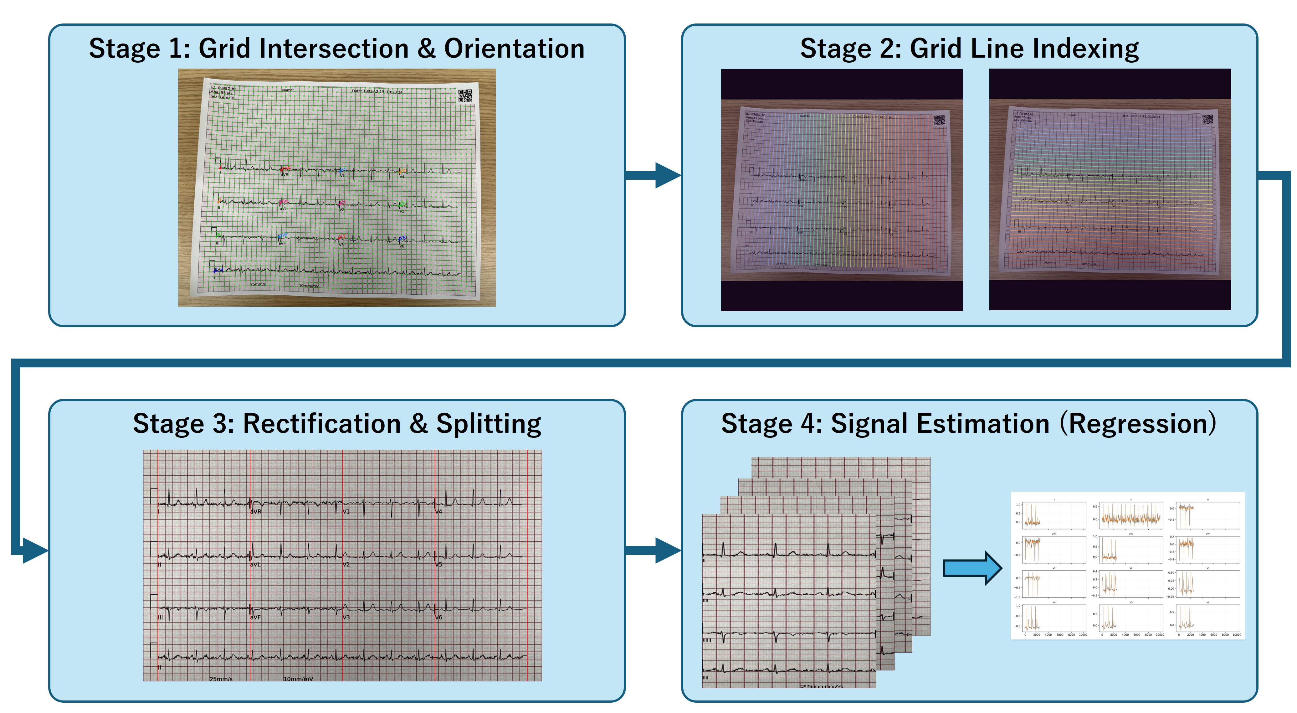\n\n### Stage 1: Grid Intersection & Orientation\n\n#### Grid Intersection & Layout Detection\nFor one high-resolution image, I use a sliding window (704x704 size, 0.5 overlap) to estimate the following using a multi-task model:\n\n1. **Grid Intersection Heatmap**: All grid intersections.\n2. **Layout Segmentation**: Positions of lead separator lines and calibration signals.\n\n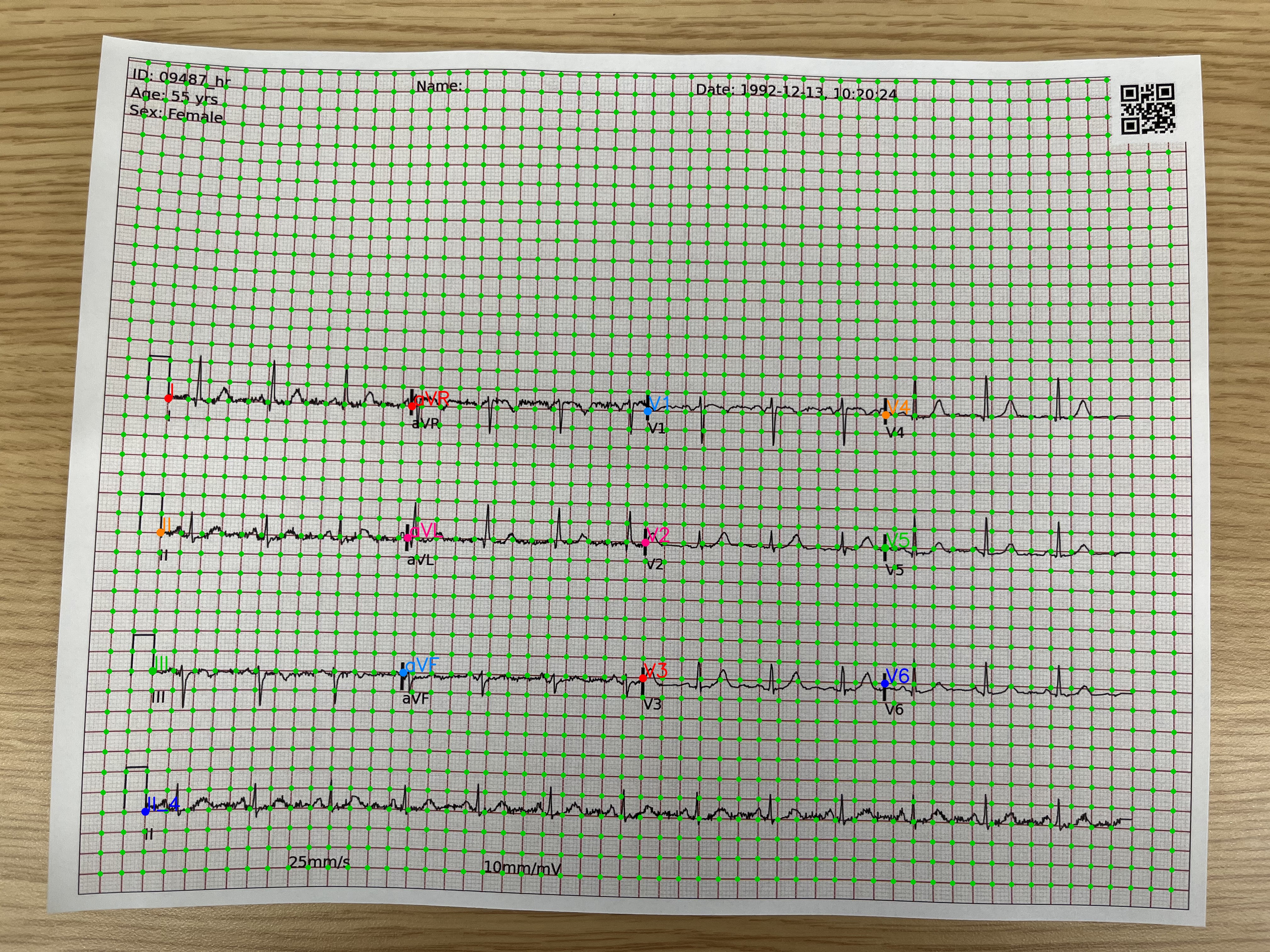\n\n#### Orientation Correction\nUsing the detected layout information, I estimate the image orientation and rotate it (0/90/180/270 degrees) to a unified upright orientation. The detected intersection coordinates are also rotated.\n\n### Stage 2: Grid Line Indexing\n\nUsing the corrected image, the model estimates an index for each pixel indicating which vertical or horizontal line it belongs to.\n\n- **Input**: Resized and padded to 1536x1536.\n- **Output**: Vertical line index (55 classes + background), Horizontal line index (43 classes + background).\n- **Assignment**: For each intersection detected in Stage 1, I aggregate the predicted labels in its neighborhood (radius 6px) and determine the row/col index by majority vote.\n\nThis determines where each intersection corresponds to in the grid `(row, col)`.\n\n### Stage 3: Rectification & Splitting\n\n#### Rectification (Grid Unwarping)\nI create a sampling coordinate field from the indexed intersections and warp the image to a fixed-size coordinate system. This method is the same as the `grid_sample` approach shared by @hengck23.\nThe output size is fixed at 1700x2200.\n\n#### Crop & Vertical Splitting\nThe rectified image often contains headers or margins, so I crop the top 25% to keep only the signal area.\nThen, I split the image width into **4 segments**. The segment boundaries are determined by converting fixed column indices to pixels in the rectified image.\n\n- Each segment contains 3 short leads and 2.5 seconds of the long Lead II stacked vertically.\n- **Purpose**:\n - **Reduce Complexity**: The model does not need to search spatially for where each lead is in the whole image.\n - **Information Interpolation**: Since the time axis is aligned within the same segment, taking 4 signals as input allows the model to use information from signals above and below to fill in gaps if grid lines are missing or noisy.\n\nEach segment image is resized to 800x800.\n\n### Stage 4: Signal Estimation (Regression)\n\n#### Waveform Estimation Model\nThe model takes the 4 segmented images as input and regresses the time-series values for 12 leads.\n\n- **Input**: 800x800 x 3ch (x 4 segments)\n- **Output**:\n - **Short Leads**: Outputs waveforms for the corresponding 3 leads from each of the 4 segments.\n - **Long Lead II**: Concatenates features from the 4 segments and outputs the full-length waveform.\n- **Resampling**: The fixed-length output sequence is resampled to the required number of samples based on the test data's `fs` (sampling frequency) using linear interpolation.\n\n#### Ensemble\nI trained multiple models with different backbones and ensembled them using weighted median. The median was more robust against spike-like outlier predictions than the mean.\n\n| Backbone | Weight | CV (SNR) | Public LB | Private LB |\n|---|---:|---:|---:|---:|\n| resnetaa101d.sw_in12k_ft_in1k | 1 | 25.62 | 21.99 | 22.03 |\n| tf_efficientnetv2_m.in21k_ft_in1k | 3 | 26.05 | 22.39 | 22.42 |\n| tf_efficientnet_b6.ns_jft_in1k | 4 | 26.05 | 22.50 | 22.44 |\n| tf_efficientnetv2_l.in21k_ft_in1k | 2 | 26.08 | 22.50 | 22.53 |\n| Ensemble (Mean) | | 26.58 | 22.30 | 22.37 |\n| Ensemble (Median) | | 26.45 | **22.71** | **22.69** |\n\n---\n\n## Models & Training Strategy\n\n### Stage 1 & 2 Models (Grid & Index)\n\n#### Dataset & Annotation\nI created annotations (intersections and line indices) myself. I used a cycle of \"Initial labeling by rule-based processing\" -> \"Model training\" -> \"Manual correction of inference results\" to create about 1000 annotated images. Note that \"lines\" are stored as sequences of intersections, not as pixel-level continuous curves.\n\n#### Backbone & Pretraining\nI used ConvNeXt Small (`convnext_small.dinov3_lvd1689m`) for the backbones of Stage 1 and 2.\nNotably, I performed pretraining in the ECG image domain using FCMAE (Fully Convolutional Masked Autoencoder). This helped the model converge faster and improved detection accuracy even with limited labels.\n\n### Stage 4 Model (Digitization)\n\n#### Network Architecture\nI used a U-Net based architecture with specific modifications for ECG Digitization.\n\n- **Asymmetric Decoder**:\n The decoder performs normal 2D Upsampling initially. However, after the feature map size becomes large enough (1/8 scale), it performs Upsampling only in the horizontal (time) direction.\n - This reduces the computational cost of unnecessary vertical resolution while ensuring high temporal resolution.\n- **Multi-head Regression**:\n - **Short Leads Head**: Performs Global Average Pooling vertically on the decoder output, then regresses using 1D Conv.\n - **Long Lead II Head**: Concatenates features between segments along the time axis, then regresses using another 1D Conv.\n- **Auxiliary Head**:\n I added a segmentation head to estimate the signal area for each lead. This was an auxiliary task to improve signal discrimination.\n\n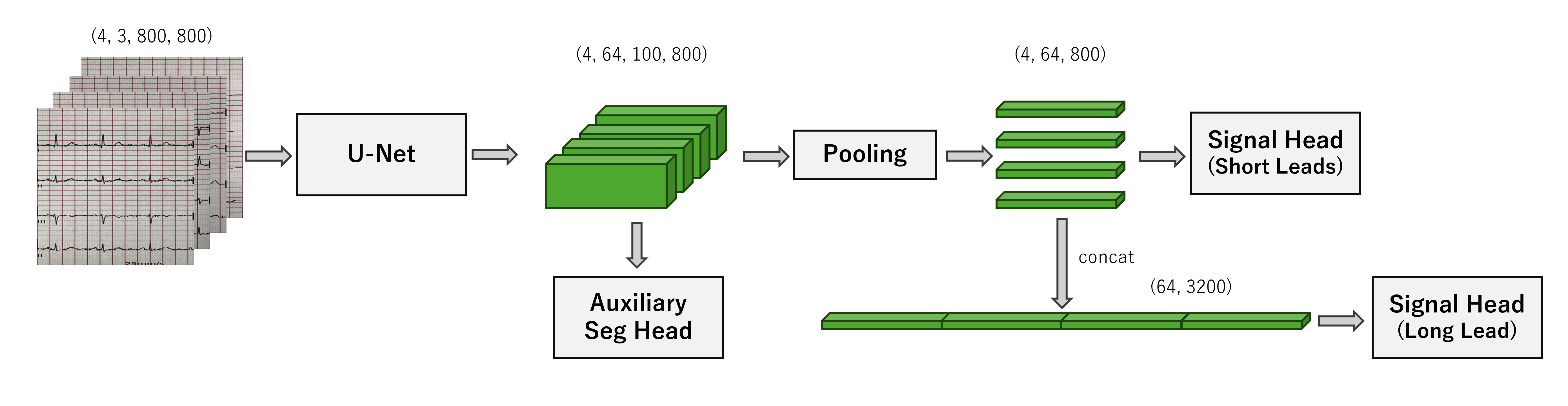\n\n#### Loss Function\nTo prevent discrepancy with the evaluation metric, I designed a loss function based on SNR. I optimized the SNR term and the Mean term separately.\n\n#### External Datasets\nIn addition to the training data, I used the following external datasets converted into images using `ecg-image-kit`:\n- PTB-XL\n- CODE-15%\n\nSince the generated data has accurate ground truth masks for which pixel corresponds to which lead, I was able to use them for training the auxiliary segmentation task.\n\n---\n\n## References\n\n1. Woo, S., Debnath, S., Hu, R., Chen, X., Liu, Z., Kweon, I. S., & Xie, S. (2023). Convnext v2: Co-designing and scaling convnets with masked autoencoders. In Proceedings of the IEEE/CVF conference on computer vision and pattern recognition (pp. 16133-16142).\n\n1. Kshama Kodthalu Shivashankara, Deepanshi, Afagh Mehri Shervedani, Matthew A. Reyna, Gari D. Clifford, Reza Sameni (2024). ECG-image-kit: a synthetic image generation toolbox to facilitate deep learning-based electrocardiogram digitization. In Physiological Measurement. IOP Publishing. doi: 10.1088/1361-6579/ad4954\n\n1. ECG-Image-Kit: A Toolkit for Synthesis, Analysis, and Digitization of Electrocardiogram Images, (2024). URL: https://github.com/alphanumericslab/ecg-image-kit\n\n1. Wagner, P., Strodthoff, N., Bousseljot, R., Samek, W., & Schaeffter, T. (2022). PTB-XL, a large publicly available electrocardiography dataset (version 1.0.3). PhysioNet. RRID:SCR_007345. https://doi.org/10.13026/kfzx-aw45\n\n1. Ribeiro, A. H., Paixao, G. M. M., Lima, E. M., Horta Ribeiro, M., Pinto Filho, M. M., Gomes, P. R., Oliveira, D. M., Meira Jr, W., Schon, T. B., & Ribeiro, A. L. P. (2021). CODE-15%: a large scale annotated dataset of 12-lead ECGs (1.0.0) [Data set]. Zenodo. https://doi.org/10.5281/zenodo.4916206\n\n## Code Release\n\nCode: https://github.com/uchiyama33/physionet_4th_place\n\nSubmission notebook: https://www.kaggle.com/code/tomoon33/physionet-submission-4th-place", "votes": null }, { "id": "3398690", "postDate": "01/29/2026 14:48:56", "content": "Congrats on the win I was going through your git hub code trying to reproduce the work, but got stuck with a missing json file error. data/annotations/multitask_lines_v2/. could you update that or provide resources to reproduce that file
", "rawMarkdown": "Congrats on the win I was going through your git hub code trying to reproduce the work, but got stuck with a missing json file error. data/annotations/multitask_lines_v2/. could you update that or provide resources to reproduce that file", "votes": null }, { "id": "3398714", "postDate": "01/29/2026 15:36:12", "content": "Thanks for checking out the code. I’ve uploaded the missing annotation files to GitHub under data/annotations/. Please pull the latest commit and try again.
", "rawMarkdown": "Thanks for checking out the code. I’ve uploaded the missing annotation files to GitHub under data/annotations/. Please pull the latest commit and try again.", "votes": null }, { "id": "3490238", "postDate": "07/06/2026 06:55:55", "content": "hi, @tomoon33 . what type of GPU did u use to train it and how long did it take?\nCongrats on this amazing work btw.
", "rawMarkdown": "hi, @tomoon33 . what type of GPU did u use to train it and how long did it take?\nCongrats on this amazing work btw.", "votes": null } ], "comments": [ { "id": 3398690, "author_name": "cartoonistbeard", "author_url": "", "post_date": "01/29/2026 14:48:56", "content": "Congrats on the win I was going through your git hub code trying to reproduce the work, but got stuck with a missing json file error. data/annotations/multitask_lines_v2/. could you update that or provide resources to reproduce that file
", "votes": null, "replies": [ { "id": 3398714, "author_name": "tomoon33", "author_url": "", "post_date": "01/29/2026 15:36:12", "content": "Thanks for checking out the code. I’ve uploaded the missing annotation files to GitHub under data/annotations/. Please pull the latest commit and try again.
", "votes": null, "replies": [] } ] }, { "id": 3490238, "author_name": "beckpro", "author_url": "", "post_date": "07/06/2026 06:55:55", "content": "hi, @tomoon33 . what type of GPU did u use to train it and how long did it take?\nCongrats on this amazing work btw.
", "votes": null, "replies": [] } ], "raw_markdown_by_id": { "3396403": "First, I would like to thank the hosts and Kaggle for organizing this competition.\nI will explain my 4th place solution, focusing on the processing pipeline and model/training strategy.\n\n## Solution Overview\n\nMy approach focuses on rectification to make it easier for the model to recognize the signals, and then estimating the waveform using a regression model. Signal segmentation is treated only as an auxiliary task.\n\nThe main points are:\n\n- **Robust Rectification**: Estimate grid intersections and layout, then map from an indexed grid to a normalized coordinate system (based on @hengck23's Discussion).\n- **Vertical Splitting**: Split the rectified image vertically by leads. This reduces the complexity of the prediction task.\n- **SNR-based Training**: Use a loss function based on SNR, which is close to the evaluation metric.\n\n---\n\n## Processing Pipeline\n\nThe process from input image to signal estimation is divided into 4 stages.\n\n\n\n### Stage 1: Grid Intersection & Orientation\n\n#### Grid Intersection & Layout Detection\nFor one high-resolution image, I use a sliding window (704x704 size, 0.5 overlap) to estimate the following using a multi-task model:\n\n1. **Grid Intersection Heatmap**: All grid intersections.\n2. **Layout Segmentation**: Positions of lead separator lines and calibration signals.\n\n\n\n#### Orientation Correction\nUsing the detected layout information, I estimate the image orientation and rotate it (0/90/180/270 degrees) to a unified upright orientation. The detected intersection coordinates are also rotated.\n\n### Stage 2: Grid Line Indexing\n\nUsing the corrected image, the model estimates an index for each pixel indicating which vertical or horizontal line it belongs to.\n\n- **Input**: Resized and padded to 1536x1536.\n- **Output**: Vertical line index (55 classes + background), Horizontal line index (43 classes + background).\n- **Assignment**: For each intersection detected in Stage 1, I aggregate the predicted labels in its neighborhood (radius 6px) and determine the row/col index by majority vote.\n\nThis determines where each intersection corresponds to in the grid `(row, col)`.\n\n### Stage 3: Rectification & Splitting\n\n#### Rectification (Grid Unwarping)\nI create a sampling coordinate field from the indexed intersections and warp the image to a fixed-size coordinate system. This method is the same as the `grid_sample` approach shared by @hengck23.\nThe output size is fixed at 1700x2200.\n\n#### Crop & Vertical Splitting\nThe rectified image often contains headers or margins, so I crop the top 25% to keep only the signal area.\nThen, I split the image width into **4 segments**. The segment boundaries are determined by converting fixed column indices to pixels in the rectified image.\n\n- Each segment contains 3 short leads and 2.5 seconds of the long Lead II stacked vertically.\n- **Purpose**:\n - **Reduce Complexity**: The model does not need to search spatially for where each lead is in the whole image.\n - **Information Interpolation**: Since the time axis is aligned within the same segment, taking 4 signals as input allows the model to use information from signals above and below to fill in gaps if grid lines are missing or noisy.\n\nEach segment image is resized to 800x800.\n\n### Stage 4: Signal Estimation (Regression)\n\n#### Waveform Estimation Model\nThe model takes the 4 segmented images as input and regresses the time-series values for 12 leads.\n\n- **Input**: 800x800 x 3ch (x 4 segments)\n- **Output**:\n - **Short Leads**: Outputs waveforms for the corresponding 3 leads from each of the 4 segments.\n - **Long Lead II**: Concatenates features from the 4 segments and outputs the full-length waveform.\n- **Resampling**: The fixed-length output sequence is resampled to the required number of samples based on the test data's `fs` (sampling frequency) using linear interpolation.\n\n#### Ensemble\nI trained multiple models with different backbones and ensembled them using weighted median. The median was more robust against spike-like outlier predictions than the mean.\n\n| Backbone | Weight | CV (SNR) | Public LB | Private LB |\n|---|---:|---:|---:|---:|\n| resnetaa101d.sw_in12k_ft_in1k | 1 | 25.62 | 21.99 | 22.03 |\n| tf_efficientnetv2_m.in21k_ft_in1k | 3 | 26.05 | 22.39 | 22.42 |\n| tf_efficientnet_b6.ns_jft_in1k | 4 | 26.05 | 22.50 | 22.44 |\n| tf_efficientnetv2_l.in21k_ft_in1k | 2 | 26.08 | 22.50 | 22.53 |\n| Ensemble (Mean) | | 26.58 | 22.30 | 22.37 |\n| Ensemble (Median) | | 26.45 | **22.71** | **22.69** |\n\n---\n\n## Models & Training Strategy\n\n### Stage 1 & 2 Models (Grid & Index)\n\n#### Dataset & Annotation\nI created annotations (intersections and line indices) myself. I used a cycle of \"Initial labeling by rule-based processing\" -> \"Model training\" -> \"Manual correction of inference results\" to create about 1000 annotated images. Note that \"lines\" are stored as sequences of intersections, not as pixel-level continuous curves.\n\n#### Backbone & Pretraining\nI used ConvNeXt Small (`convnext_small.dinov3_lvd1689m`) for the backbones of Stage 1 and 2.\nNotably, I performed pretraining in the ECG image domain using FCMAE (Fully Convolutional Masked Autoencoder). This helped the model converge faster and improved detection accuracy even with limited labels.\n\n### Stage 4 Model (Digitization)\n\n#### Network Architecture\nI used a U-Net based architecture with specific modifications for ECG Digitization.\n\n- **Asymmetric Decoder**:\n The decoder performs normal 2D Upsampling initially. However, after the feature map size becomes large enough (1/8 scale), it performs Upsampling only in the horizontal (time) direction.\n - This reduces the computational cost of unnecessary vertical resolution while ensuring high temporal resolution.\n- **Multi-head Regression**:\n - **Short Leads Head**: Performs Global Average Pooling vertically on the decoder output, then regresses using 1D Conv.\n - **Long Lead II Head**: Concatenates features between segments along the time axis, then regresses using another 1D Conv.\n- **Auxiliary Head**:\n I added a segmentation head to estimate the signal area for each lead. This was an auxiliary task to improve signal discrimination.\n\n\n\n#### Loss Function\nTo prevent discrepancy with the evaluation metric, I designed a loss function based on SNR. I optimized the SNR term and the Mean term separately.\n\n#### External Datasets\nIn addition to the training data, I used the following external datasets converted into images using `ecg-image-kit`:\n- PTB-XL\n- CODE-15%\n\nSince the generated data has accurate ground truth masks for which pixel corresponds to which lead, I was able to use them for training the auxiliary segmentation task.\n\n---\n\n## References\n\n1. Woo, S., Debnath, S., Hu, R., Chen, X., Liu, Z., Kweon, I. S., & Xie, S. (2023). Convnext v2: Co-designing and scaling convnets with masked autoencoders. In Proceedings of the IEEE/CVF conference on computer vision and pattern recognition (pp. 16133-16142).\n\n1. Kshama Kodthalu Shivashankara, Deepanshi, Afagh Mehri Shervedani, Matthew A. Reyna, Gari D. Clifford, Reza Sameni (2024). ECG-image-kit: a synthetic image generation toolbox to facilitate deep learning-based electrocardiogram digitization. In Physiological Measurement. IOP Publishing. doi: 10.1088/1361-6579/ad4954\n\n1. ECG-Image-Kit: A Toolkit for Synthesis, Analysis, and Digitization of Electrocardiogram Images, (2024). URL: https://github.com/alphanumericslab/ecg-image-kit\n\n1. Wagner, P., Strodthoff, N., Bousseljot, R., Samek, W., & Schaeffter, T. (2022). PTB-XL, a large publicly available electrocardiography dataset (version 1.0.3). PhysioNet. RRID:SCR_007345. https://doi.org/10.13026/kfzx-aw45\n\n1. Ribeiro, A. H., Paixao, G. M. M., Lima, E. M., Horta Ribeiro, M., Pinto Filho, M. M., Gomes, P. R., Oliveira, D. M., Meira Jr, W., Schon, T. B., & Ribeiro, A. L. P. (2021). CODE-15%: a large scale annotated dataset of 12-lead ECGs (1.0.0) [Data set]. Zenodo. https://doi.org/10.5281/zenodo.4916206\n\n## Code Release\n\nCode: https://github.com/uchiyama33/physionet_4th_place\n\nSubmission notebook: https://www.kaggle.com/code/tomoon33/physionet-submission-4th-place", "3398690": "Congrats on the win I was going through your git hub code trying to reproduce the work, but got stuck with a missing json file error. data/annotations/multitask_lines_v2/. could you update that or provide resources to reproduce that file", "3398714": "Thanks for checking out the code. I’ve uploaded the missing annotation files to GitHub under data/annotations/. Please pull the latest commit and try again.", "3490238": "hi, @tomoon33 . what type of GPU did u use to train it and how long did it take?\nCongrats on this amazing work btw." }, "source": "meta" }