
Our best submission works by running three separate solutions, then computing a weighted average of their predictions. We formed our team late in the competition, so our pipelines were developed with relatively few shared assumptions. This independence increased model diversity, thereby allowing our ensemble to significantly outperform the individual scores.
\n| Solution | \nEnsemble Weight | \nPublic LB Score | \nPrivate LB Score | \n
|---|---|---|---|
| Imanishi's pipeline | \n45% | \n21.58 | \n21.43 | \n
| James's pipeline | \n32% | \n21.17 | \n20.98 | \n
| Liu's pipeline | \n23% | \n20.84 | \n20.74 | \n
| Ensemble | \nN/A | \n22.16 | \n22.03 | \n
At a high level, all of our solutions work by rectifying the input images to correct for distortions, then using segmentation models and softmax operations to extract the voltage signals. However, there were some substantial differences in our preprocessing methodology (1-stage vs. 2-stage), model architectures (CNNs vs. Transformers), segmentation loss functions (binary cross entropy vs. custom \"coord\" loss), and signal post-processing methodology (anomaly suppression techniques & signal sharpening transforms). As a result, the inaccuracies in our predictions are largely uncorrelated and weighted averaging improves the signal to noise ratio substantially.
\nOur individual solutions are described in greater detail below.
\nUsing hengck23’s excellent notebook as a baseline, I introduced the following improvements:
\nReplaced the stage0 model with my own trained model.\nThe original motivation was to completely exclude pretrained data when computing CV scores, but since it also improved the LB score, I adopted it. (Stage1 ultimately remains hengck23’s model.)
When converting to rectified input images for stage2, hengck23 performed the transformation in two steps. To reduce image quality degradation, I instead computed a grid from the outputs of stage0 and stage1 and transformed the original image in a single step using F.grid_sample().
Increased the stage2 input resolution, especially in the x-direction (input size: 1632 × 4480).
Introduced the Coord loss idea from my teammate liuzhangzhen into stage2.
Added y-direction clustering–based masking in stage2.
Instead of filling low-confidence predictions in stage2 with 0 mV, I switched to linear interpolation.
Adopted EfficientNetV2B1-UNet for the stage0 and stage2 models (it is unclear how much this contributed to accuracy).
Added the following post-processing:
\nsavgol_filter with a dynamically adjusted window_length depending on sig_len.In Liu’s implementation of Coord loss, both the segmentation loss and the Coord loss are applied to the same logits. In my case, this did not work well, so I split the model head into two heads (segmentation head, y-coordinate head) and applied segmentation loss (dice loss + BCE loss) and Coord loss separately.
\nBoth heads have the same output shape: [height, width, 4ch].
\nThe segmentation loss acts like an auxiliary loss during training, but the segmentation output is also used during inference for masking low-confidence regions in the x-direction and for the y-clustering described later.
\nAlthough Liu’s section already explains Coord Loss, I will describe what I consider important.
\nWith a segmentation-based approach like hengck23’s baseline, where the curve mask is predicted and then argmax is used to obtain y-coordinates, it is difficult to estimate optimal y positions. This becomes clear when looking at the ground truth for the two heads (following figure).
With Coord Loss, the logits output (height × width × 4 channels) are the same as in segmentation head up to a point, but then a softmax over the y-dimension is applied to directly predict the y-coordinate.
\nIf we use a one-hot label with only one pixel as ground truth, the model becomes very sensitive to small coordinate shifts. Instead, the ground truth is represented as a Gaussian-shaped probability distribution along the y-axis. The Gaussian parameters (sigma and radius) were kept the same as Liu’s because I did not have time to tune them.
\nThe loss function is standard cross-entropy loss, treating the problem as multi-class classification over y positions.
\nBy applying argmax along the y-direction on the Coord Loss head output, we can obtain much more accurate y-coordinates. Adding Coord Loss improved my public LB score by about +1.0 dB, which is a large gain.
For some reason, my stage2 model occasionally misclassified lead labels, which could significantly degrade the SNR. I wanted to prevent this during training, but in the end I could not, so I handled it with a post-processing step using y-direction clustering.
\nFor y-clustering, I used the output from the segmentation head, and the generated masks were then applied to the y-coordinate head.
\n
In the submission notebook, I split the entire test set into two parts and assigned one T4 GPU to each process, as shown in the code below, in order to speed up inference.
\nIn practice, my part of the pipeline runs in about 70 minutes, which was the fastest among the team members.
\nenv1 = os.environ.copy()\nenv2 = os.environ.copy()\nenv1['CUDA_VISIBLE_DEVICES'] = '0'\nenv2['CUDA_VISIBLE_DEVICES'] = '1'\n\ncmd1 = f'python run.py --half 0'\nproc1 = subprocess.Popen(cmd1.split(' '), env=env1)\n\ncmd2 = f'python run.py --half 1'\nproc2 = subprocess.Popen(cmd2.split(' '), env=env2)\n\n_ = proc1.communicate()\n_ = proc2.communicate()\nMy inference pipeline has 3 main steps:
\nSteps 1 and 2 both use finetuned versions of DINOv2-base. I used an ensemble of 6 models in total, 2 in step 1, 4 in step 2. Half of the models process the images in an intentionally flipped orientation as a form of test time data augmentation.
\nI generated ~175K training examples based on ~22K unique ECG records from the PTB-XL dataset.
\nThis was done by generating \"clean\" ECG images with ECG-image-kit, then intentionally corrupting them with some custom data augmentation code which tries to roughly imitate they types of images that appear in the host's data (cell phone pictures of paper with heavy damage, cell phone pictures of computer screens, black and white scans, etc).
\nEach image type was roughly simulated using a combination of the following (in no particular order):
\nAdditional augmentations were performed on-the-fly in my training scripts, those are just the ones I applied before training.
\nOf the ~175K extra training examples, only ~50K were used to train my final models. Primarily because (1) the accuracy of the keypoint detectors didn't seem to meaningfully improve beyond ~17K training examples and (2) the gains from pretraining the lead segmentation models on synthetic data before finetuning on the host images was pretty small relative to the amount of GPU time it was consuming (a little over two RTX 5090 days of extra compute for a +0.17 dB gain was a bit disappointing… I wanted to try other things instead of having my hardware tied up pushing further in that direction).
\nThis works by detecting keypoints in the images, then using those keypoint locations to compute a homography matrix that can be used to correct for differences in camera angle, zoom, and rotation. It is fairly similar to @hengck23's stage 0, with the main differences being that I used a vision transformer instead of a CNN and training data that I generated myself.
\n
Keypoints were detected at a resolution of 1036x1036, then used to directly rectify images from their native resolutions --> 1694x2198.
\nTraining details:
\nalbumentations):RandomRotate90GridDistortionElasticTransformOpticalDistortionGaussNoiseGaussianBlurRandomBrightnessContrastColorJitterCoarseDropoutBoth of the keypoint detection models in my final ensemble were trained on 17.4K of my synthetic training examples (and none of the host data). They primarily differed in the data agmentation settings & training epoch count. One was trained with moderately heavy agumentation & 24 epochs, the other was trained with heavier augmentation & 48 epochs.
\nTripling the training data to ~50K examples improved cross validation when testing against other synthetic images, but did not improve the scores of my full pipeline when testing against the ECG images provided by the host, so only ~10% of the available synthetic data was used to train the keypoint detectors in my final ensemble.
\nI used the ground-truth signal data to generate \"perfect\" heatmaps describing where the leads ought to be located in the images if they were completely undistored, then finetuned DINOv2-base to predict those heatmaps based on images with realistic distortions. This teaches it to automatically correct for any warping which makes it past my preprocessing.
\n
I found it very beneficial to use horizontal resolutions higher than the native resolution of the ECG plots, so this uses an input resolution of 1694x4396 (~2x wider than native) and I inserted a ConvTranspose2d layer between the transformer backbone and the prediction head, which increased resolution another 2x shortly before producing the outputs. As a result, the heatmaps have a resolution of 1694x8792. This provided MASSIVE score improvements in comparison to just using the naive resolution, roughly a 4.1 dB gain in early experiments. Using an input resolution 2x higher than native and output resolution 4x higher than native appeared to be ~optimal, adjusting either of those figures by a factor of 2 makes the score worse.
Training took place in 2 stages:
\nTraining details:
\nA.GridDistortion(num_steps=5, distort_limit=0.2, p=0.15) during pretraining and didn't have any explicit data augmentation during finetuning. However, finetuning intentionally used rectified images from an older, less accurate, version of my preprocessing pipeline, so models are exposed to more rectification errors during training than they are at test time. Using more accurate rectification for the training data makes my scores worse, so I believe rectification inaccuracies act as a form of sneaky data augmentation during finetuning.My pipeline rectifies each image twice using separate keypoint detection models, then flips one of the resulting images and feeds them to a collection of 4 lead segmentation models, half of which were trained to process images in the flipped orientation. The resulting heatmaps were then blended by averaging the pixel logits.
\n
The approach above is based on the following observations:
\nThe score could likely be improved further by processing the images in more orientations, applying some of the test time augmentations unrelated to rotation & flipping from other top solutions & public notebooks, and figuring out why applying TTA before rectification didn't help (maybe I had a bug?), but I didn't have time to experiment with this super extensively.
\nI convert the raw predicted lead location heatmaps to signals via the following steps:
\n… as usual, many of the things that don't work well for me could potentially work well with additional effort and GPU time for tuning. I frequently move on to testing other ideas when early results don't seem promising. Many of the \"bad\" ideas above wound up working well for other top competitors 😅
\nI would like to express my sincere gratitude to Kaggle and the competition organizers for providing this invaluable opportunity. Special thanks to @hengck23 for sharing his strong baseline, which served as a crucial foundation for my work.
\nMy solution optimizes Stage 2 of @hengck23’s baseline. The key insight is to treat waveform extraction as per-column coordinate regression, rather than relying purely on a “segmentation → post-processing” pipeline.
\nI keep the U-Net–style heatmap prediction for stability, but add CoordLoss: a GT-centered local Gaussian cross-entropy that directly supervises the centerline y-coordinate per column. On my local validation split, this single change improved SNR by more than +1 dB, and it was the dominant contributor to overall quality.
\nTo further reduce train–inference mismatch, validation/inference uses the same old-subpixel-compatible y extractor (NaN + interpolation behavior). I also add lightweight “safe” regularizers enforcing physically plausible lead relationships.
\nStage 0/1 (baseline): detect and rectify ECG sheets into canonical coordinates (rectified strips).
\nStage 2 (this work):
\nModel: ResNet34 encoder + U-Net decoder → 4 heatmaps (3 short rows + long Lead II).
Losses:
\nInference:
\nArchitecture
\ntimm resnet34.a3_in1kBatchNorm freezing\nAll BN layers are forced into eval mode during training, which stabilizes optimization under batch size 1 with gradient accumulation.
\nLosses
\nMasked Pixel BCE (baseline supervision)\nI rasterize GT polylines into thin heatmap masks and apply BCEWithLogitsLoss, masked by valid columns. Since the final metric is strongly influenced by the rhythm strip, I upweight Long Lead II (via channel weighting and/or multiplicity depending on the run).
CoordLoss (main gain, +1 dB)\nMotivation: segmentation-style BCE does not directly optimize the quantity we ultimately need—the centerline y-coordinate per column. Even small vertical errors can degrade SNR after alignment and interpolation.
Method: for each channel c and valid column x
\nTreat logits over height as a categorical distribution:
\nBuild a GT-centered local Gaussian target around the continuous ground-truth (y^*(x,c)):
\nCompute cross-entropy using log-softmax values in that local window (local Gaussian CE)
This provides dense, well-shaped gradients for precise localization, even when the line is thin or partially missing. In ablations, CoordLoss produced the largest improvement and drove the overall gain.
\nThese are intentionally lightweight; they mainly help avoid implausible outputs and reduce boundary artifacts, while CoordLoss provides the primary accuracy boost.
\nWe ensemble our predictions by:
\nThis provided a gain of 0.6 dB over our best individual submission 😁.
", "messages": [ { "id": "3395990", "postDate": "01/24/2026 04:31:00", "content": "Our best submission works by running three separate solutions, then computing a weighted average of their predictions. We formed our team late in the competition, so our pipelines were developed with relatively few shared assumptions. This independence increased model diversity, thereby allowing our ensemble to significantly outperform the individual scores.
\n| Solution | \nEnsemble Weight | \nPublic LB Score | \nPrivate LB Score | \n
|---|---|---|---|
| Imanishi's pipeline | \n45% | \n21.58 | \n21.43 | \n
| James's pipeline | \n32% | \n21.17 | \n20.98 | \n
| Liu's pipeline | \n23% | \n20.84 | \n20.74 | \n
| Ensemble | \nN/A | \n22.16 | \n22.03 | \n
At a high level, all of our solutions work by rectifying the input images to correct for distortions, then using segmentation models and softmax operations to extract the voltage signals. However, there were some substantial differences in our preprocessing methodology (1-stage vs. 2-stage), model architectures (CNNs vs. Transformers), segmentation loss functions (binary cross entropy vs. custom \"coord\" loss), and signal post-processing methodology (anomaly suppression techniques & signal sharpening transforms). As a result, the inaccuracies in our predictions are largely uncorrelated and weighted averaging improves the signal to noise ratio substantially.
\nOur individual solutions are described in greater detail below.
\nUsing hengck23’s excellent notebook as a baseline, I introduced the following improvements:
\nReplaced the stage0 model with my own trained model.\nThe original motivation was to completely exclude pretrained data when computing CV scores, but since it also improved the LB score, I adopted it. (Stage1 ultimately remains hengck23’s model.)
When converting to rectified input images for stage2, hengck23 performed the transformation in two steps. To reduce image quality degradation, I instead computed a grid from the outputs of stage0 and stage1 and transformed the original image in a single step using F.grid_sample().
Increased the stage2 input resolution, especially in the x-direction (input size: 1632 × 4480).
Introduced the Coord loss idea from my teammate liuzhangzhen into stage2.
Added y-direction clustering–based masking in stage2.
Instead of filling low-confidence predictions in stage2 with 0 mV, I switched to linear interpolation.
Adopted EfficientNetV2B1-UNet for the stage0 and stage2 models (it is unclear how much this contributed to accuracy).
Added the following post-processing:
\nsavgol_filter with a dynamically adjusted window_length depending on sig_len.In Liu’s implementation of Coord loss, both the segmentation loss and the Coord loss are applied to the same logits. In my case, this did not work well, so I split the model head into two heads (segmentation head, y-coordinate head) and applied segmentation loss (dice loss + BCE loss) and Coord loss separately.
\nBoth heads have the same output shape: [height, width, 4ch].
\nThe segmentation loss acts like an auxiliary loss during training, but the segmentation output is also used during inference for masking low-confidence regions in the x-direction and for the y-clustering described later.
\nAlthough Liu’s section already explains Coord Loss, I will describe what I consider important.
\nWith a segmentation-based approach like hengck23’s baseline, where the curve mask is predicted and then argmax is used to obtain y-coordinates, it is difficult to estimate optimal y positions. This becomes clear when looking at the ground truth for the two heads (following figure).
With Coord Loss, the logits output (height × width × 4 channels) are the same as in segmentation head up to a point, but then a softmax over the y-dimension is applied to directly predict the y-coordinate.
\nIf we use a one-hot label with only one pixel as ground truth, the model becomes very sensitive to small coordinate shifts. Instead, the ground truth is represented as a Gaussian-shaped probability distribution along the y-axis. The Gaussian parameters (sigma and radius) were kept the same as Liu’s because I did not have time to tune them.
\nThe loss function is standard cross-entropy loss, treating the problem as multi-class classification over y positions.
\nBy applying argmax along the y-direction on the Coord Loss head output, we can obtain much more accurate y-coordinates. Adding Coord Loss improved my public LB score by about +1.0 dB, which is a large gain.
For some reason, my stage2 model occasionally misclassified lead labels, which could significantly degrade the SNR. I wanted to prevent this during training, but in the end I could not, so I handled it with a post-processing step using y-direction clustering.
\nFor y-clustering, I used the output from the segmentation head, and the generated masks were then applied to the y-coordinate head.
\n
In the submission notebook, I split the entire test set into two parts and assigned one T4 GPU to each process, as shown in the code below, in order to speed up inference.
\nIn practice, my part of the pipeline runs in about 70 minutes, which was the fastest among the team members.
\nenv1 = os.environ.copy()\nenv2 = os.environ.copy()\nenv1['CUDA_VISIBLE_DEVICES'] = '0'\nenv2['CUDA_VISIBLE_DEVICES'] = '1'\n\ncmd1 = f'python run.py --half 0'\nproc1 = subprocess.Popen(cmd1.split(' '), env=env1)\n\ncmd2 = f'python run.py --half 1'\nproc2 = subprocess.Popen(cmd2.split(' '), env=env2)\n\n_ = proc1.communicate()\n_ = proc2.communicate()\nMy inference pipeline has 3 main steps:
\nSteps 1 and 2 both use finetuned versions of DINOv2-base. I used an ensemble of 6 models in total, 2 in step 1, 4 in step 2. Half of the models process the images in an intentionally flipped orientation as a form of test time data augmentation.
\nI generated ~175K training examples based on ~22K unique ECG records from the PTB-XL dataset.
\nThis was done by generating \"clean\" ECG images with ECG-image-kit, then intentionally corrupting them with some custom data augmentation code which tries to roughly imitate they types of images that appear in the host's data (cell phone pictures of paper with heavy damage, cell phone pictures of computer screens, black and white scans, etc).
\nEach image type was roughly simulated using a combination of the following (in no particular order):
\nAdditional augmentations were performed on-the-fly in my training scripts, those are just the ones I applied before training.
\nOf the ~175K extra training examples, only ~50K were used to train my final models. Primarily because (1) the accuracy of the keypoint detectors didn't seem to meaningfully improve beyond ~17K training examples and (2) the gains from pretraining the lead segmentation models on synthetic data before finetuning on the host images was pretty small relative to the amount of GPU time it was consuming (a little over two RTX 5090 days of extra compute for a +0.17 dB gain was a bit disappointing… I wanted to try other things instead of having my hardware tied up pushing further in that direction).
\nThis works by detecting keypoints in the images, then using those keypoint locations to compute a homography matrix that can be used to correct for differences in camera angle, zoom, and rotation. It is fairly similar to @hengck23's stage 0, with the main differences being that I used a vision transformer instead of a CNN and training data that I generated myself.
\n
Keypoints were detected at a resolution of 1036x1036, then used to directly rectify images from their native resolutions --> 1694x2198.
\nTraining details:
\nalbumentations):RandomRotate90GridDistortionElasticTransformOpticalDistortionGaussNoiseGaussianBlurRandomBrightnessContrastColorJitterCoarseDropoutBoth of the keypoint detection models in my final ensemble were trained on 17.4K of my synthetic training examples (and none of the host data). They primarily differed in the data agmentation settings & training epoch count. One was trained with moderately heavy agumentation & 24 epochs, the other was trained with heavier augmentation & 48 epochs.
\nTripling the training data to ~50K examples improved cross validation when testing against other synthetic images, but did not improve the scores of my full pipeline when testing against the ECG images provided by the host, so only ~10% of the available synthetic data was used to train the keypoint detectors in my final ensemble.
\nI used the ground-truth signal data to generate \"perfect\" heatmaps describing where the leads ought to be located in the images if they were completely undistored, then finetuned DINOv2-base to predict those heatmaps based on images with realistic distortions. This teaches it to automatically correct for any warping which makes it past my preprocessing.
\n
I found it very beneficial to use horizontal resolutions higher than the native resolution of the ECG plots, so this uses an input resolution of 1694x4396 (~2x wider than native) and I inserted a ConvTranspose2d layer between the transformer backbone and the prediction head, which increased resolution another 2x shortly before producing the outputs. As a result, the heatmaps have a resolution of 1694x8792. This provided MASSIVE score improvements in comparison to just using the naive resolution, roughly a 4.1 dB gain in early experiments. Using an input resolution 2x higher than native and output resolution 4x higher than native appeared to be ~optimal, adjusting either of those figures by a factor of 2 makes the score worse.
Training took place in 2 stages:
\nTraining details:
\nA.GridDistortion(num_steps=5, distort_limit=0.2, p=0.15) during pretraining and didn't have any explicit data augmentation during finetuning. However, finetuning intentionally used rectified images from an older, less accurate, version of my preprocessing pipeline, so models are exposed to more rectification errors during training than they are at test time. Using more accurate rectification for the training data makes my scores worse, so I believe rectification inaccuracies act as a form of sneaky data augmentation during finetuning.My pipeline rectifies each image twice using separate keypoint detection models, then flips one of the resulting images and feeds them to a collection of 4 lead segmentation models, half of which were trained to process images in the flipped orientation. The resulting heatmaps were then blended by averaging the pixel logits.
\n
The approach above is based on the following observations:
\nThe score could likely be improved further by processing the images in more orientations, applying some of the test time augmentations unrelated to rotation & flipping from other top solutions & public notebooks, and figuring out why applying TTA before rectification didn't help (maybe I had a bug?), but I didn't have time to experiment with this super extensively.
\nI convert the raw predicted lead location heatmaps to signals via the following steps:
\n… as usual, many of the things that don't work well for me could potentially work well with additional effort and GPU time for tuning. I frequently move on to testing other ideas when early results don't seem promising. Many of the \"bad\" ideas above wound up working well for other top competitors 😅
\nI would like to express my sincere gratitude to Kaggle and the competition organizers for providing this invaluable opportunity. Special thanks to @hengck23 for sharing his strong baseline, which served as a crucial foundation for my work.
\nMy solution optimizes Stage 2 of @hengck23’s baseline. The key insight is to treat waveform extraction as per-column coordinate regression, rather than relying purely on a “segmentation → post-processing” pipeline.
\nI keep the U-Net–style heatmap prediction for stability, but add CoordLoss: a GT-centered local Gaussian cross-entropy that directly supervises the centerline y-coordinate per column. On my local validation split, this single change improved SNR by more than +1 dB, and it was the dominant contributor to overall quality.
\nTo further reduce train–inference mismatch, validation/inference uses the same old-subpixel-compatible y extractor (NaN + interpolation behavior). I also add lightweight “safe” regularizers enforcing physically plausible lead relationships.
\nStage 0/1 (baseline): detect and rectify ECG sheets into canonical coordinates (rectified strips).
\nStage 2 (this work):
\nModel: ResNet34 encoder + U-Net decoder → 4 heatmaps (3 short rows + long Lead II).
Losses:
\nInference:
\nArchitecture
\ntimm resnet34.a3_in1kBatchNorm freezing\nAll BN layers are forced into eval mode during training, which stabilizes optimization under batch size 1 with gradient accumulation.
\nLosses
\nMasked Pixel BCE (baseline supervision)\nI rasterize GT polylines into thin heatmap masks and apply BCEWithLogitsLoss, masked by valid columns. Since the final metric is strongly influenced by the rhythm strip, I upweight Long Lead II (via channel weighting and/or multiplicity depending on the run).
CoordLoss (main gain, +1 dB)\nMotivation: segmentation-style BCE does not directly optimize the quantity we ultimately need—the centerline y-coordinate per column. Even small vertical errors can degrade SNR after alignment and interpolation.
Method: for each channel c and valid column x
\nTreat logits over height as a categorical distribution:
\nBuild a GT-centered local Gaussian target around the continuous ground-truth (y^*(x,c)):
\nCompute cross-entropy using log-softmax values in that local window (local Gaussian CE)
This provides dense, well-shaped gradients for precise localization, even when the line is thin or partially missing. In ablations, CoordLoss produced the largest improvement and drove the overall gain.
\nThese are intentionally lightweight; they mainly help avoid implausible outputs and reduce boundary artifacts, while CoordLoss provides the primary accuracy boost.
\nWe ensemble our predictions by:
\nThis provided a gain of 0.6 dB over our best individual submission 😁.
", "rawMarkdown": "# Overview\n\nOur best submission works by running three separate solutions, then computing a weighted average of their predictions. We formed our team late in the competition, so our pipelines were developed with relatively few shared assumptions. This independence increased model diversity, thereby allowing our ensemble to significantly outperform the individual scores.\n\n| Solution | Ensemble Weight | Public LB Score | Private LB Score |\n| -------- | --------------- | --------------- | ---------------- |\n| Imanishi's pipeline | 45% | 21.58 | 21.43 |\n| James's pipeline | 32% | 21.17 | 20.98 |\n| Liu's pipeline | 23% | 20.84 | 20.74 |\n| Ensemble | N/A | 22.16 | 22.03 |\n\nAt a high level, all of our solutions work by rectifying the input images to correct for distortions, then using segmentation models and softmax operations to extract the voltage signals. However, there were some substantial differences in our preprocessing methodology (1-stage vs. 2-stage), model architectures (CNNs vs. Transformers), segmentation loss functions (binary cross entropy vs. custom \"coord\" loss), and signal post-processing methodology (anomaly suppression techniques & signal sharpening transforms). As a result, the inaccuracies in our predictions are largely uncorrelated and weighted averaging improves the signal to noise ratio substantially.\n\nOur individual solutions are described in greater detail below.\n\n# Imanishi's Pipeline\n\n### Overview of Imanishi's Part\n\nUsing [hengck23’s excellent notebook](https://www.kaggle.com/code/hengck23/demo-submission) as a baseline, I introduced the following improvements:\n\n* Replaced the stage0 model with my own trained model.\n The original motivation was to completely exclude pretrained data when computing CV scores, but since it also improved the LB score, I adopted it. (Stage1 ultimately remains hengck23’s model.)\n* When converting to rectified input images for stage2, hengck23 performed the transformation in two steps. To reduce image quality degradation, I instead computed a grid from the outputs of stage0 and stage1 and transformed the original image in a single step using `F.grid_sample()`.\n* Increased the stage2 input resolution, especially in the x-direction (input size: **1632 × 4480**).\n* Introduced the **Coord loss** idea from my teammate liuzhangzhen into stage2.\n* Added y-direction clustering–based masking in stage2.\n* Instead of filling low-confidence predictions in stage2 with 0 mV, I switched to **linear interpolation**.\n* Adopted **EfficientNetV2B1-UNet** for the stage0 and stage2 models (it is unclear how much this contributed to accuracy).\n* Added the following post-processing:\n\n * Correction of Leads I, II, and III using **Einthoven’s law**.\n * Since the first quarter of Lead II overlaps with two waveforms, apply average ensembling.\n * Apply `savgol_filter` with a dynamically adjusted `window_length` depending on `sig_len`.\n\n\n\n### Details of Stage2 Model\n\nIn Liu’s implementation of Coord loss, both the segmentation loss and the Coord loss are applied to the same logits. In my case, this did not work well, so I split the model head into two heads (segmentation head, y-coordinate head) and applied **segmentation loss (dice loss + BCE loss)** and **Coord loss** separately.\n\nBoth heads have the same output shape: [height, width, 4ch].\n\nThe segmentation loss acts like an auxiliary loss during training, but the segmentation output is also used during inference for masking low-confidence regions in the x-direction and for the y-clustering described later.\n\n\n\n### Coord Loss\n\nAlthough Liu’s section already explains Coord Loss, I will describe what I consider important.\n\nWith a segmentation-based approach like hengck23’s baseline, where the curve mask is predicted and then `argmax` is used to obtain y-coordinates, it is difficult to estimate optimal y positions. This becomes clear when looking at the ground truth for the two heads (following figure).\n\nWith Coord Loss, the logits output (**height × width × 4 channels**) are the same as in segmentation head up to a point, but then a **softmax over the y-dimension** is applied to directly predict the y-coordinate.\n\nIf we use a one-hot label with only one pixel as ground truth, the model becomes very sensitive to small coordinate shifts. Instead, the ground truth is represented as a **Gaussian-shaped probability distribution** along the y-axis. The Gaussian parameters (sigma and radius) were kept the same as Liu’s because I did not have time to tune them.\n\nThe loss function is standard **cross-entropy loss**, treating the problem as multi-class classification over y positions.\n\nBy applying `argmax` along the y-direction on the Coord Loss head output, we can obtain much more accurate y-coordinates. Adding Coord Loss improved my public LB score by about **+1.0 dB**, which is a large gain.\n\n[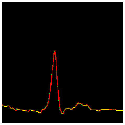](https://postimg.cc/p59nH9h1)\n\n\n### Y-Clustering\n\nFor some reason, my stage2 model occasionally misclassified lead labels, which could significantly degrade the SNR. I wanted to prevent this during training, but in the end I could not, so I handled it with a **post-processing step using y-direction clustering**.\n\nFor y-clustering, I used the output from the segmentation head, and the generated masks were then applied to the y-coordinate head.\n\n[](https://postimg.cc/JtXg1pNv)\n\n\n### Other Tricks\n\nIn the submission notebook, I split the entire test set into two parts and assigned one T4 GPU to each process, as shown in the code below, in order to speed up inference.\n\nIn practice, my part of the pipeline runs in about **70 minutes**, which was the fastest among the team members.\n\n```python\nenv1 = os.environ.copy()\nenv2 = os.environ.copy()\nenv1['CUDA_VISIBLE_DEVICES'] = '0'\nenv2['CUDA_VISIBLE_DEVICES'] = '1'\n\ncmd1 = f'python run.py --half 0'\nproc1 = subprocess.Popen(cmd1.split(' '), env=env1)\n\ncmd2 = f'python run.py --half 1'\nproc2 = subprocess.Popen(cmd2.split(' '), env=env2)\n\n_ = proc1.communicate()\n_ = proc2.communicate()\n```\n\n# James's Pipeline\n### Overview\nMy inference pipeline has 3 main steps:\n1. **Preprocessing:** Detect landmarks in the images and use them to correct for affine warping (such as camera perspective variations & rotation, but not wrinkles in the paper).\n2. **Lead segmentation:** Predict a heatmap describing where the leads hypothetically would be located if the input image was perfectly \"clean\" and undistorted. This is better at handling \"natural\" distortions than unnatural ones caused by imperfect non-affine warp correction, so attempting to correct for non-affine warping with preprocessing logic similar to [@hengck23](https://www.kaggle.com/hengck23)'s baseline is harmful in my pipeline.\n3. **Heatmap-to-signal conversion:** I use top-k softmax operations to predict estimated voltages & confidence intervals for each lead at each timestep, replace extremely low confidence predictions with ones interpolated from context, use a top-hat transform to \"sharpen\" the remaining voltage spikes, and use a little linear algebra to exploit redundancy between leads for denoising purposes.\n\nSteps 1 and 2 both use finetuned versions of [DINOv2-base](https://huggingface.co/timm/vit_base_patch14_reg4_dinov2.lvd142m). I used an ensemble of 6 models in total, 2 in step 1, 4 in step 2. Half of the models process the images in an intentionally flipped orientation as a form of test time data augmentation.\n\n### Data generation\n\nI generated ~175K training examples based on ~22K unique ECG records from the PTB-XL dataset.\n\nThis was done by generating \"clean\" ECG images with [ECG-image-kit](https://github.com/alphanumericslab/ecg-image-kit/tree/main/codes/ecg-image-generator), then intentionally corrupting them with some custom data augmentation code which tries to roughly imitate they types of images that appear in the host's data (cell phone pictures of paper with heavy damage, cell phone pictures of computer screens, black and white scans, etc). \n\nEach image type was roughly simulated using a combination of the following (in no particular order):\n* **Affine warping**\n* **Background image insertion:** For simulated cellphone pics, the warped ECG images were overlaid on top of images from [unsplash-25k](https://www.kaggle.com/datasets/ntsv648/unsplash-25k). For scanner pics, I used a white background.\n* **Stain insertion:** This works by overlaying translucent mold and stain images on top of the ECG images. The stains were randomly drawn from a pool of 26 that I generated semi-manually by prompting a diffusion model. In hindsight, I think the stain intensity distribution I used was a bit unrealistic (typically too transparent) and wonder if maybe pwelin noise would work better than the stain images I generated, but never got around to tinkering with a second version of this.\n* **Wrinkle shading:** This simulates the shadows from hypothetical wrinkles without introducing any non-affine warping. It is very similar to functionality from ECG-image-kit, I just had ChatGPT port it into my script.\n* **Black-and-white scanner simulation:** This ain't an off the shelf greyscale conversion. I tried to simulate the behavior of black and white scanners by randomizing brightness, contrast, gamma, and the way the input color channels are weighted. It also injects a little gaussian noise to mimic sensor noise & quantization artifacts.\n\nAdditional augmentations were performed on-the-fly in my training scripts, those are just the ones I applied before training.\n\nOf the ~175K extra training examples, only ~50K were used to train my final models. Primarily because (1) the accuracy of the keypoint detectors didn't seem to meaningfully improve beyond ~17K training examples and (2) the gains from pretraining the lead segmentation models on synthetic data before finetuning on the host images was pretty small relative to the amount of GPU time it was consuming (a little over two RTX 5090 days of extra compute for a +0.17 dB gain was a bit disappointing... I wanted to try other things instead of having my hardware tied up pushing further in that direction).\n\n### Camera perspective correction\n\nThis works by detecting keypoints in the images, then using those keypoint locations to compute a homography matrix that can be used to correct for differences in camera angle, zoom, and rotation. It is fairly similar to @hengck23's stage 0, with the main differences being that I used a vision transformer instead of a CNN and training data that I generated myself.\n\n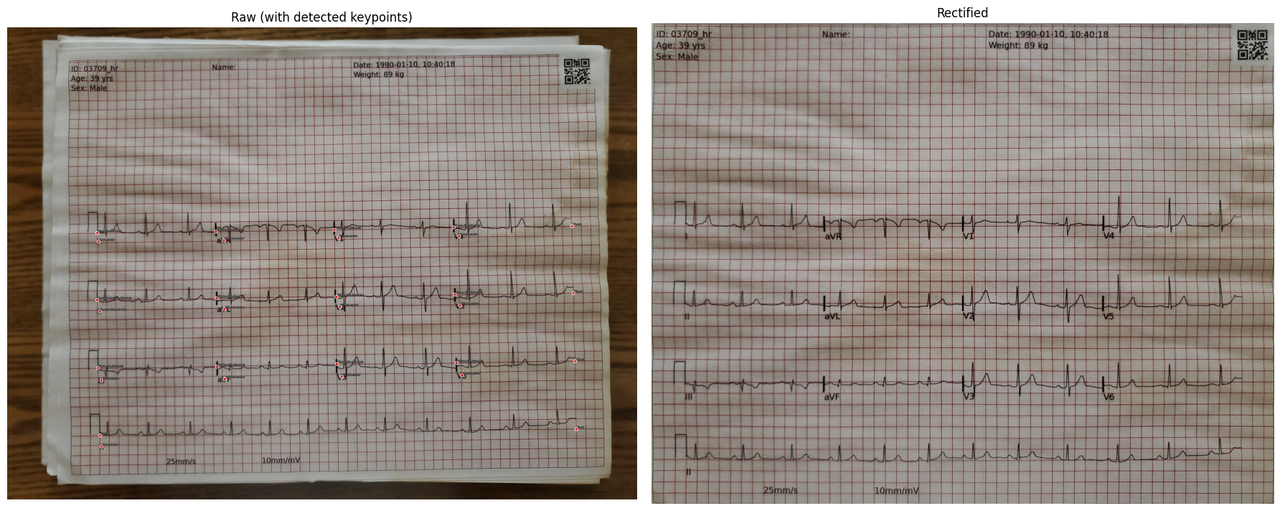\n\nKeypoints were detected at a resolution of 1036x1036, then used to directly rectify images from their native resolutions --> 1694x2198.\n\nTraining details:\n* Model architecture: DINOv2-base backbone with linear prediction head that produces 30 channel outputs (1 per target landmark, all lead label text + the start and end of each signal's x axis).\n* Trained to imitate ground truth heatmaps with 1 \"gaussian blob\" per keypoint. These blobs have a value of 1 in the center and decay towards zero as distance from the center increases.\n* BCE loss\n* AdamW optimizer\n* One-cycle learning rate schedule\n* Data augmentations (applied using `albumentations`):\n * `RandomRotate90`\n * `GridDistortion`\n * `ElasticTransform`\n * `OpticalDistortion`\n * `GaussNoise`\n * `GaussianBlur`\n * `RandomBrightnessContrast`\n * `ColorJitter`\n * `CoarseDropout`\n\nBoth of the keypoint detection models in my final ensemble were trained on 17.4K of my synthetic training examples (and none of the host data). They primarily differed in the data agmentation settings & training epoch count. One was trained with moderately heavy agumentation & 24 epochs, the other was trained with heavier augmentation & 48 epochs.\n\nTripling the training data to ~50K examples improved cross validation when testing against other synthetic images, but did not improve the scores of my full pipeline when testing against the ECG images provided by the host, so only ~10% of the available synthetic data was used to train the keypoint detectors in my final ensemble.\n\n### Lead segmentation\n\nI used the ground-truth signal data to generate \"perfect\" heatmaps describing where the leads ought to be located in the images if they were completely undistored, then finetuned DINOv2-base to predict those heatmaps based on images with realistic distortions. This teaches it to automatically correct for any warping which makes it past my preprocessing.\n\n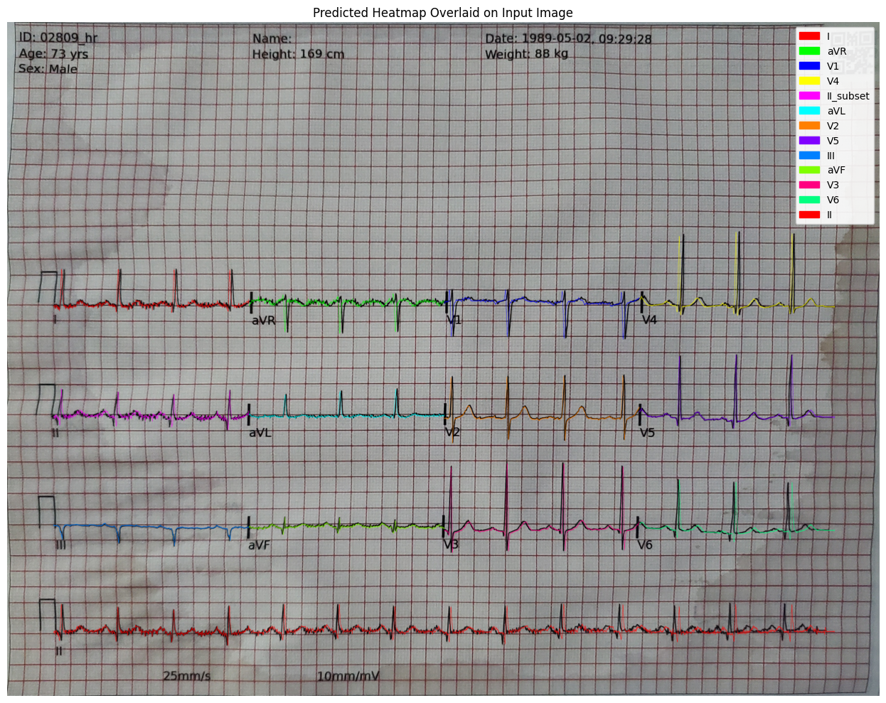\n\nI found it very beneficial to use horizontal resolutions higher than the native resolution of the ECG plots, so this uses an input resolution of 1694x4396 (~2x wider than native) and I inserted a `ConvTranspose2d` layer between the transformer backbone and the prediction head, which increased resolution another 2x shortly before producing the outputs. As a result, the heatmaps have a resolution of **1694x8792**. This provided **MASSIVE score improvements in comparison to just using the naive resolution, roughly a 4.1 dB gain** in early experiments. Using an input resolution 2x higher than native and output resolution 4x higher than native appeared to be ~optimal, adjusting either of those figures by a factor of 2 makes the score worse.\n\nTraining took place in 2 stages:\n1. Pretraining on my synthetic images\n2. Finetuning on the host images\n\nTraining details:\n* **Data:** Stage 1 used 17.4K synthetic images per model with different images used for each model in the ensemble. Stage 2 used 80% of the host data, with 20% held in reserve for cross-validation.\n* **Mask generation:** Unlike the keypoint detection models, I found it beneficial for the ground-truth segmentation masks used to train these models to be very sharp. The ground-truth lead lines are only a single pixel thick with no blur.\n* **Activation checkpointing:** Training vision transformers at high resolutions uses a lot of memory. I used [activation checkpointing](https://pytorch.org/blog/activation-checkpointing-techniques/) to mitigate this. It allows for a configurable tradeoff between speed and memory usage. I found the speed drawbacks to be extremely minor. It can cut memory usage in half with almost zero slowdown.\n* **Data augmentation:** Aggressive data augmentation seems to do more harm than good for these models, so I used relatively light configs. For most models in the ensemble, I just used `A.GridDistortion(num_steps=5, distort_limit=0.2, p=0.15)` during pretraining and didn't have any *explicit* data augmentation during finetuning. However, finetuning intentionally used rectified images from an older, less accurate, version of my preprocessing pipeline, so models are exposed to more rectification errors during training than they are at test time. Using more accurate rectification for the training data makes my scores worse, so I believe rectification inaccuracies act as a form of sneaky data augmentation during finetuning.\n* **Loss functions:** 3 of the 4 lead segmentation models in my ensemble were just trained to minimize binary cross entropy loss. One of them used a hybrid loss during finetuning in which it also tries to minimize the mean squared error of the predicted y pixel coordinates at each timestep. That seemed to be *slightly* beneficial (0.05 dB in cross validation, even less on the leaderboard), but I didn't have time to propagate it to all models in the ensemble. Applying L1 or L2 losses like that is something which consistently did more harm than good to me earlier in the competition, so I initially abandoned it, but it seemed somewhat beneficial after the pretraining was added; I think pretraining purely with BCE before adding MSE or MAE helps to prevent much of the overfitting & instability I encountered earlier.\n* **Misc:** AdamW optimizer & one cycle learning rate scheduler, similar to the keypoint detector.\n\n### Test time augmentation & ensembling\n\nMy pipeline rectifies each image twice using separate keypoint detection models, then flips one of the resulting images and feeds them to a collection of 4 lead segmentation models, half of which were trained to process images in the flipped orientation. The resulting heatmaps were then blended by averaging the pixel logits.\n\n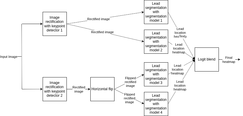\n\nThe approach above is based on the following observations:\n1. Averaging predictions from models in the standard & flipped orientations provides a gain of roughly 0.28 dB.\n2. Using 2 lead segmentation models per orientation provides a gain of roughly 0.18 dB.\n3. Using 2 models for rectification (instead of 1) provides a gain of roughly 0.13 dB.\n4. Averaging the pixel logits scores ~0.02 dB better than averaging after signal extraction.\n5. Flipping or rotating the images before rectification does not help.\n\nThe score could likely be improved further by processing the images in more orientations, applying some of the test time augmentations unrelated to rotation & flipping from other top solutions & public notebooks, and figuring out why applying TTA before rectification didn't help (maybe I had a bug?), but I didn't have time to experiment with this super extensively.\n\n### Signal extraction & post processing\nI convert the raw predicted lead location heatmaps to signals via the following steps:\n1. **Heatmap --> raw signal:** Within each column of the image where a lead is expected to be located (based on the canonical layout), I use a top-k softmax to compute the estimated probability of the lead being located at each vertical pixel coordinate, then use those probability estimates to compute the expected signal value. Using a top-k softmax with k=10 scored ~0.28 dB better than using a hard argmax. I tried k ∈ {3, 5, 10, 20, unlimited} and found 5 & 10 to be roughly tied for \"best\". The optimal choice varies by model depending on minor differences in other hyperparameters.\n2. **Unconfident prediction replacement:** The top-k softmax operations are also used to compute upper and lower confidence bounds for the signal values at each timestep. If those bounds are more than 0.4 mV apart, the sample is dropped and the gaps are filled in by linearly interpolating from the surrounding context samples. The range covered by the confidence interval corresponds to either the top-10 most likely vertical pixel coordinates or the min and max pixel coordinates with associated probability estimates above 0.1%, whichever is narrower for each timestep. This provided a gain of roughly 0.13 dB in comparison to a baseline without confidence filtering.\n3. **Edge artifact suppression:** I remove edge artifacts by replacing the rightmost 2 voltage samples for each lead with the one located 3rd from the right. The rightmost samples tend to be inaccurate because the \"ground truth\" training signals contain some voltage spikes that are not visible in the printed images, which causes the model to be prone to hallucinating at the end. Partially suppressing those errors gave me a ~0.05 dB gain (some of them leak through this filtering, a 2px safety margin is not wide enough to fully eliminate them).\n4. **Signal sharpening:** The peaks of the voltage spikes tend to be a bit \"rounded\" due to the input images having lower resolution than the raw signals they're based on, so a [top-hat transform](https://en.wikipedia.org/wiki/Top-hat_transform) is used to sharpen them. This provided a gain of roughly 0.04 dB. It worked better for me than sharpening with a shock filter (+0.01 dB gain in CV, did not test on LB) or 1D unsharp masking (harmful in CV, did not test on LB).\n5. **I/II/III redundancy exploitation (einthoven's law):** This takes place in several stages. First, the I and III leads are aligned with II to correct for small timing discrepancies. Then the II = I + III relation (einthoven's law) is used to compute \"expected\" signal values for each of those 3 leads based on the other two. Finally, the raw extracted signals are blended with their expected values via weighted averaging with two thirds of the weight assigned to the raw values. This provides a gain of roughly 0.05 dB. It was critically important to align the signals first, otherwise this is harmful for me. I also tried exploiting the aVR + aVL + aVF = 0 relation in a similar manner, and observed a similar gain in local cross validation from doing so, but unlike I/II/III the aV* post processing did not work well on the leaderboard, so my final pipeline only does einthoven post-processing for I/II/III.\n6. **II & rhythm strip redundancy exploitation:** The II signal appears twice in each image, once as a 2.5 second segment, then again as a 10 second segment (rhythm strip) whose prefix should match the shorter segment. My II predictions are generated by aligning the shorter signal with the longer one (correcting for small timing discrepancies), then computing a weighted average with ~56% of the weight given to the long signal, ~44% given to the shorter one. This provides a gain of roughly 0.01 dB... barely measurable, but was consistent for both CV & LB.\n7. **Sample rate adjustment:** Signals are re-sampled to match the host's desired sample rates via linear interpolation. I also tried cubic, akima spline, and PCHIP interpolation, but linear worked best.\n\n### Things that didn't work well for me\n* Correcting for non-affine image warping during preprocessing\n* DeepLabV3 segmentation models\n* Larger DINO v2 models\n* DINO v3\n* Post-processing with 1D CNNs\n* Using differentiable warping operations so that the preprocessing model(s) can be trained end-to-end with the final lead segmentation model\n\n... as usual, many of the things that don't work well for me could potentially work well with additional effort and GPU time for tuning. I frequently move on to testing other ideas when early results don't seem promising. Many of the \"bad\" ideas above wound up working well for other top competitors 😅\n\n# Liu's Pipeline\n\n### Acknowledgments\n\nI would like to express my sincere gratitude to Kaggle and the competition organizers for providing this invaluable opportunity. Special thanks to @hengck23 for sharing his strong baseline, which served as a crucial foundation for my work.\n\n### Summary\n\nMy solution optimizes Stage 2 of @hengck23’s baseline. The key insight is to treat waveform extraction as **per-column coordinate regression**, rather than relying purely on a “segmentation → post-processing” pipeline.\n\nI keep the U-Net–style heatmap prediction for stability, but add **CoordLoss**: a GT-centered **local Gaussian cross-entropy** that directly supervises the centerline y-coordinate per column. On my local validation split, this single change improved SNR by **more than +1 dB**, and it was the dominant contributor to overall quality.\n\nTo further reduce train–inference mismatch, validation/inference uses the same **old-subpixel-compatible y extractor** (NaN + interpolation behavior). I also add lightweight “safe” regularizers enforcing physically plausible lead relationships.\n\n### Overall Pipeline\n\nStage 0/1 (baseline): detect and rectify ECG sheets into canonical coordinates (rectified strips).\n\nStage 2 (this work):\n\n* Model: ResNet34 encoder + U-Net decoder → **4 heatmaps** (3 short rows + long Lead II).\n* Losses:\n\n * Masked BCE (heatmap supervision)\n * **CoordLoss (main gain)**\n * Small auxiliary losses (consistency + lead relationships)\n* Inference:\n\n * Predict full-width logits\n * Logits → y(px) using the same old-subpixel extraction as validation (NaN → interpolation)\n * Convert y(px) → mV\n * Apply Einthoven-based patching for long Lead II near the boundary\n\n### Stage 2 Model\n\nArchitecture\n\n* Encoder: `timm resnet34.a3_in1k`\n* Decoder: U-Net style decoder (MyCoordUnetDecoder) with multi-scale skip connections\n* Head: 1×1 conv → 4 heatmaps\n\nBatchNorm freezing\nAll BN layers are forced into eval mode during training, which stabilizes optimization under batch size 1 with gradient accumulation.\n\nLosses\n\n1. Masked Pixel BCE (baseline supervision)\n I rasterize GT polylines into thin heatmap masks and apply BCEWithLogitsLoss, masked by valid columns. Since the final metric is strongly influenced by the rhythm strip, I upweight **Long Lead II** (via channel weighting and/or multiplicity depending on the run).\n\n2. CoordLoss (main gain, +1 dB)\n Motivation: segmentation-style BCE does not directly optimize the quantity we ultimately need—**the centerline y-coordinate per column**. Even small vertical errors can degrade SNR after alignment and interpolation.\n\nMethod: for each channel c and valid column x\n\n* Treat logits over height as a categorical distribution:\n\n * ( p(y\\mid x,c)=\\mathrm{softmax}(z_c[:,x]/T) )\n* Build a GT-centered local Gaussian target around the continuous ground-truth (y^*(x,c)):\n\n * ( w_k \\propto \\exp(-(k-y^*)^2/(2\\sigma^2)) ) within a window ±R\n* Compute cross-entropy using log-softmax values in that local window (local Gaussian CE)\n\nThis provides dense, well-shaped gradients for precise localization, even when the line is thin or partially missing. In ablations, CoordLoss produced the largest improvement and drove the overall gain.\n\n3. Auxiliary “safe” regularizers (small weights)\n\n* Short II vs Long II dy consistency: applied only on segment0 (Short II time), using SmoothL1 on centered dy to reduce drift/slope mismatch.\n* Einthoven bridge (mV domain): encourage Long II near the boundary to match an Einthoven-corrected (II_{\\text{corr}}=(1-w),II+w,(I+III)), with warmup/ramp for stability.\n* Lead relationship penalty (hinge): enforce (II \\approx I + III) on segment0 using a tolerance-based squared hinge.\n\nThese are intentionally lightweight; they mainly help avoid implausible outputs and reduce boundary artifacts, while CoordLoss provides the primary accuracy boost.\n\n# Ensembling Approach\n\nWe ensemble our predictions by:\n1. Aligning the signals to correct for minor time discrepancies that would otherwise act as a blur filter if the signals were naively averaged together. This is done using code copied from the evaluation metric, very similar to how it aligns signals with the ground truth.\n2. Computing a weighted average of the predictions. We only did 2 submissions to try tuning the weights, so they're primarily based on rough guesswork, i.e. the assumption that the optimal weight for each pipeline's predictions would probably be correlated with its public LB score. Using weights which lean more heavily in that direction scored better than using relatively even weights (on both the public & private leaderboard), so that assumption appears to have been correct.\n\nThis provided a gain of 0.6 dB over our best individual submission 😁.", "votes": null }, { "id": "3396049", "postDate": "01/24/2026 07:19:47", "content": "Congrats @jsday96 @dimanishi @liuzhangzhen
", "rawMarkdown": "Congrats @jsday96 @dimanishi @liuzhangzhen", "votes": null }, { "id": "3396063", "postDate": "01/24/2026 07:54:07", "content": "Thanks @navneetbende
", "rawMarkdown": "Thanks @navneetbende", "votes": null }, { "id": "3396137", "postDate": "01/24/2026 12:11:01", "content": "Congratulations on the work. Could you share how you generated the ground-truth (GT) masks from the GT signals for the signal segmentation task?\nIn our case, we used plotted pixel coordinates from a JSON file generated by ECG-image-kit while regenerating image 0001 from the GT signal, and drew the signal mask with a line thickness of 1 pixel. However, even though the segmentation results looked visually good, the reconstructed signal achieved only modest SNR (around 14–15 dB). Our GT masks with resultion 1700-2200 give only 20-22 db
", "rawMarkdown": "Congratulations on the work. Could you share how you generated the ground-truth (GT) masks from the GT signals for the signal segmentation task?\nIn our case, we used plotted pixel coordinates from a JSON file generated by ECG-image-kit while regenerating image 0001 from the GT signal, and drew the signal mask with a line thickness of 1 pixel. However, even though the segmentation results looked visually good, the reconstructed signal achieved only modest SNR (around 14–15 dB). Our GT masks with resultion 1700-2200 give only 20-22 db", "votes": null }, { "id": "3396215", "postDate": "01/24/2026 14:45:28", "content": "Thank you! Each of us three used a different method, but I used matplotlib.
", "rawMarkdown": "Thank you! Each of us three used a different method, but I used matplotlib.", "votes": null }, { "id": "3396238", "postDate": "01/24/2026 15:19:29", "content": "I used cv2.polylines to generate one binary mask per lead, then stacked together those masks to form the full 13 channel target masks.
@jsday96 congratulations with GM 🎉
", "rawMarkdown": "jsday96 congratulations with GM 🎉", "votes": null }, { "id": "3396404", "postDate": "01/25/2026 00:25:50", "content": "Thanks! 🎉
", "rawMarkdown": "Thanks! 🎉", "votes": null }, { "id": "3396405", "postDate": "01/25/2026 00:33:28", "content": "I rasterize each valid centerline into a thin 4-channel binary mask by drawing the polyline on a blank canvas per channel using cv2.polylines
", "rawMarkdown": "I rasterize each valid centerline into a thin 4-channel binary mask by drawing the polyline on a blank canvas per channel using cv2.polylines", "votes": null } ], "comments": [ { "id": 3396049, "author_name": "navneetbende", "author_url": "", "post_date": "01/24/2026 07:19:47", "content": "Congrats @jsday96 @dimanishi @liuzhangzhen
", "votes": null, "replies": [ { "id": 3396063, "author_name": "liuzhangzhen", "author_url": "", "post_date": "01/24/2026 07:54:07", "content": "Thanks @navneetbende
", "votes": null, "replies": [] } ] }, { "id": 3396137, "author_name": "vandongtran", "author_url": "", "post_date": "01/24/2026 12:11:01", "content": "Congratulations on the work. Could you share how you generated the ground-truth (GT) masks from the GT signals for the signal segmentation task?\nIn our case, we used plotted pixel coordinates from a JSON file generated by ECG-image-kit while regenerating image 0001 from the GT signal, and drew the signal mask with a line thickness of 1 pixel. However, even though the segmentation results looked visually good, the reconstructed signal achieved only modest SNR (around 14–15 dB). Our GT masks with resultion 1700-2200 give only 20-22 db
", "votes": null, "replies": [ { "id": 3396215, "author_name": "dimanishi", "author_url": "", "post_date": "01/24/2026 14:45:28", "content": "Thank you! Each of us three used a different method, but I used matplotlib.
", "votes": null, "replies": [] }, { "id": 3396238, "author_name": "jsday96", "author_url": "", "post_date": "01/24/2026 15:19:29", "content": "I used cv2.polylines to generate one binary mask per lead, then stacked together those masks to form the full 13 channel target masks.
I rasterize each valid centerline into a thin 4-channel binary mask by drawing the polyline on a blank canvas per channel using cv2.polylines
", "votes": null, "replies": [] } ] }, { "id": 3396382, "author_name": "bluepill", "author_url": "", "post_date": "01/24/2026 21:28:25", "content": "@jsday96 congratulations with GM 🎉
", "votes": null, "replies": [ { "id": 3396404, "author_name": "jsday96", "author_url": "", "post_date": "01/25/2026 00:25:50", "content": "Thanks! 🎉
", "votes": null, "replies": [] } ] } ], "raw_markdown_by_id": { "3395990": "# Overview\n\nOur best submission works by running three separate solutions, then computing a weighted average of their predictions. We formed our team late in the competition, so our pipelines were developed with relatively few shared assumptions. This independence increased model diversity, thereby allowing our ensemble to significantly outperform the individual scores.\n\n| Solution | Ensemble Weight | Public LB Score | Private LB Score |\n| -------- | --------------- | --------------- | ---------------- |\n| Imanishi's pipeline | 45% | 21.58 | 21.43 |\n| James's pipeline | 32% | 21.17 | 20.98 |\n| Liu's pipeline | 23% | 20.84 | 20.74 |\n| Ensemble | N/A | 22.16 | 22.03 |\n\nAt a high level, all of our solutions work by rectifying the input images to correct for distortions, then using segmentation models and softmax operations to extract the voltage signals. However, there were some substantial differences in our preprocessing methodology (1-stage vs. 2-stage), model architectures (CNNs vs. Transformers), segmentation loss functions (binary cross entropy vs. custom \"coord\" loss), and signal post-processing methodology (anomaly suppression techniques & signal sharpening transforms). As a result, the inaccuracies in our predictions are largely uncorrelated and weighted averaging improves the signal to noise ratio substantially.\n\nOur individual solutions are described in greater detail below.\n\n# Imanishi's Pipeline\n\n### Overview of Imanishi's Part\n\nUsing [hengck23’s excellent notebook](https://www.kaggle.com/code/hengck23/demo-submission) as a baseline, I introduced the following improvements:\n\n* Replaced the stage0 model with my own trained model.\n The original motivation was to completely exclude pretrained data when computing CV scores, but since it also improved the LB score, I adopted it. (Stage1 ultimately remains hengck23’s model.)\n* When converting to rectified input images for stage2, hengck23 performed the transformation in two steps. To reduce image quality degradation, I instead computed a grid from the outputs of stage0 and stage1 and transformed the original image in a single step using `F.grid_sample()`.\n* Increased the stage2 input resolution, especially in the x-direction (input size: **1632 × 4480**).\n* Introduced the **Coord loss** idea from my teammate liuzhangzhen into stage2.\n* Added y-direction clustering–based masking in stage2.\n* Instead of filling low-confidence predictions in stage2 with 0 mV, I switched to **linear interpolation**.\n* Adopted **EfficientNetV2B1-UNet** for the stage0 and stage2 models (it is unclear how much this contributed to accuracy).\n* Added the following post-processing:\n\n * Correction of Leads I, II, and III using **Einthoven’s law**.\n * Since the first quarter of Lead II overlaps with two waveforms, apply average ensembling.\n * Apply `savgol_filter` with a dynamically adjusted `window_length` depending on `sig_len`.\n\n\n\n### Details of Stage2 Model\n\nIn Liu’s implementation of Coord loss, both the segmentation loss and the Coord loss are applied to the same logits. In my case, this did not work well, so I split the model head into two heads (segmentation head, y-coordinate head) and applied **segmentation loss (dice loss + BCE loss)** and **Coord loss** separately.\n\nBoth heads have the same output shape: [height, width, 4ch].\n\nThe segmentation loss acts like an auxiliary loss during training, but the segmentation output is also used during inference for masking low-confidence regions in the x-direction and for the y-clustering described later.\n\n\n\n### Coord Loss\n\nAlthough Liu’s section already explains Coord Loss, I will describe what I consider important.\n\nWith a segmentation-based approach like hengck23’s baseline, where the curve mask is predicted and then `argmax` is used to obtain y-coordinates, it is difficult to estimate optimal y positions. This becomes clear when looking at the ground truth for the two heads (following figure).\n\nWith Coord Loss, the logits output (**height × width × 4 channels**) are the same as in segmentation head up to a point, but then a **softmax over the y-dimension** is applied to directly predict the y-coordinate.\n\nIf we use a one-hot label with only one pixel as ground truth, the model becomes very sensitive to small coordinate shifts. Instead, the ground truth is represented as a **Gaussian-shaped probability distribution** along the y-axis. The Gaussian parameters (sigma and radius) were kept the same as Liu’s because I did not have time to tune them.\n\nThe loss function is standard **cross-entropy loss**, treating the problem as multi-class classification over y positions.\n\nBy applying `argmax` along the y-direction on the Coord Loss head output, we can obtain much more accurate y-coordinates. Adding Coord Loss improved my public LB score by about **+1.0 dB**, which is a large gain.\n\n[](https://postimg.cc/p59nH9h1)\n\n\n### Y-Clustering\n\nFor some reason, my stage2 model occasionally misclassified lead labels, which could significantly degrade the SNR. I wanted to prevent this during training, but in the end I could not, so I handled it with a **post-processing step using y-direction clustering**.\n\nFor y-clustering, I used the output from the segmentation head, and the generated masks were then applied to the y-coordinate head.\n\n[](https://postimg.cc/JtXg1pNv)\n\n\n### Other Tricks\n\nIn the submission notebook, I split the entire test set into two parts and assigned one T4 GPU to each process, as shown in the code below, in order to speed up inference.\n\nIn practice, my part of the pipeline runs in about **70 minutes**, which was the fastest among the team members.\n\n```python\nenv1 = os.environ.copy()\nenv2 = os.environ.copy()\nenv1['CUDA_VISIBLE_DEVICES'] = '0'\nenv2['CUDA_VISIBLE_DEVICES'] = '1'\n\ncmd1 = f'python run.py --half 0'\nproc1 = subprocess.Popen(cmd1.split(' '), env=env1)\n\ncmd2 = f'python run.py --half 1'\nproc2 = subprocess.Popen(cmd2.split(' '), env=env2)\n\n_ = proc1.communicate()\n_ = proc2.communicate()\n```\n\n# James's Pipeline\n### Overview\nMy inference pipeline has 3 main steps:\n1. **Preprocessing:** Detect landmarks in the images and use them to correct for affine warping (such as camera perspective variations & rotation, but not wrinkles in the paper).\n2. **Lead segmentation:** Predict a heatmap describing where the leads hypothetically would be located if the input image was perfectly \"clean\" and undistorted. This is better at handling \"natural\" distortions than unnatural ones caused by imperfect non-affine warp correction, so attempting to correct for non-affine warping with preprocessing logic similar to [@hengck23](https://www.kaggle.com/hengck23)'s baseline is harmful in my pipeline.\n3. **Heatmap-to-signal conversion:** I use top-k softmax operations to predict estimated voltages & confidence intervals for each lead at each timestep, replace extremely low confidence predictions with ones interpolated from context, use a top-hat transform to \"sharpen\" the remaining voltage spikes, and use a little linear algebra to exploit redundancy between leads for denoising purposes.\n\nSteps 1 and 2 both use finetuned versions of [DINOv2-base](https://huggingface.co/timm/vit_base_patch14_reg4_dinov2.lvd142m). I used an ensemble of 6 models in total, 2 in step 1, 4 in step 2. Half of the models process the images in an intentionally flipped orientation as a form of test time data augmentation.\n\n### Data generation\n\nI generated ~175K training examples based on ~22K unique ECG records from the PTB-XL dataset.\n\nThis was done by generating \"clean\" ECG images with [ECG-image-kit](https://github.com/alphanumericslab/ecg-image-kit/tree/main/codes/ecg-image-generator), then intentionally corrupting them with some custom data augmentation code which tries to roughly imitate they types of images that appear in the host's data (cell phone pictures of paper with heavy damage, cell phone pictures of computer screens, black and white scans, etc). \n\nEach image type was roughly simulated using a combination of the following (in no particular order):\n* **Affine warping**\n* **Background image insertion:** For simulated cellphone pics, the warped ECG images were overlaid on top of images from [unsplash-25k](https://www.kaggle.com/datasets/ntsv648/unsplash-25k). For scanner pics, I used a white background.\n* **Stain insertion:** This works by overlaying translucent mold and stain images on top of the ECG images. The stains were randomly drawn from a pool of 26 that I generated semi-manually by prompting a diffusion model. In hindsight, I think the stain intensity distribution I used was a bit unrealistic (typically too transparent) and wonder if maybe pwelin noise would work better than the stain images I generated, but never got around to tinkering with a second version of this.\n* **Wrinkle shading:** This simulates the shadows from hypothetical wrinkles without introducing any non-affine warping. It is very similar to functionality from ECG-image-kit, I just had ChatGPT port it into my script.\n* **Black-and-white scanner simulation:** This ain't an off the shelf greyscale conversion. I tried to simulate the behavior of black and white scanners by randomizing brightness, contrast, gamma, and the way the input color channels are weighted. It also injects a little gaussian noise to mimic sensor noise & quantization artifacts.\n\nAdditional augmentations were performed on-the-fly in my training scripts, those are just the ones I applied before training.\n\nOf the ~175K extra training examples, only ~50K were used to train my final models. Primarily because (1) the accuracy of the keypoint detectors didn't seem to meaningfully improve beyond ~17K training examples and (2) the gains from pretraining the lead segmentation models on synthetic data before finetuning on the host images was pretty small relative to the amount of GPU time it was consuming (a little over two RTX 5090 days of extra compute for a +0.17 dB gain was a bit disappointing... I wanted to try other things instead of having my hardware tied up pushing further in that direction).\n\n### Camera perspective correction\n\nThis works by detecting keypoints in the images, then using those keypoint locations to compute a homography matrix that can be used to correct for differences in camera angle, zoom, and rotation. It is fairly similar to @hengck23's stage 0, with the main differences being that I used a vision transformer instead of a CNN and training data that I generated myself.\n\n\n\nKeypoints were detected at a resolution of 1036x1036, then used to directly rectify images from their native resolutions --> 1694x2198.\n\nTraining details:\n* Model architecture: DINOv2-base backbone with linear prediction head that produces 30 channel outputs (1 per target landmark, all lead label text + the start and end of each signal's x axis).\n* Trained to imitate ground truth heatmaps with 1 \"gaussian blob\" per keypoint. These blobs have a value of 1 in the center and decay towards zero as distance from the center increases.\n* BCE loss\n* AdamW optimizer\n* One-cycle learning rate schedule\n* Data augmentations (applied using `albumentations`):\n * `RandomRotate90`\n * `GridDistortion`\n * `ElasticTransform`\n * `OpticalDistortion`\n * `GaussNoise`\n * `GaussianBlur`\n * `RandomBrightnessContrast`\n * `ColorJitter`\n * `CoarseDropout`\n\nBoth of the keypoint detection models in my final ensemble were trained on 17.4K of my synthetic training examples (and none of the host data). They primarily differed in the data agmentation settings & training epoch count. One was trained with moderately heavy agumentation & 24 epochs, the other was trained with heavier augmentation & 48 epochs.\n\nTripling the training data to ~50K examples improved cross validation when testing against other synthetic images, but did not improve the scores of my full pipeline when testing against the ECG images provided by the host, so only ~10% of the available synthetic data was used to train the keypoint detectors in my final ensemble.\n\n### Lead segmentation\n\nI used the ground-truth signal data to generate \"perfect\" heatmaps describing where the leads ought to be located in the images if they were completely undistored, then finetuned DINOv2-base to predict those heatmaps based on images with realistic distortions. This teaches it to automatically correct for any warping which makes it past my preprocessing.\n\n\n\nI found it very beneficial to use horizontal resolutions higher than the native resolution of the ECG plots, so this uses an input resolution of 1694x4396 (~2x wider than native) and I inserted a `ConvTranspose2d` layer between the transformer backbone and the prediction head, which increased resolution another 2x shortly before producing the outputs. As a result, the heatmaps have a resolution of **1694x8792**. This provided **MASSIVE score improvements in comparison to just using the naive resolution, roughly a 4.1 dB gain** in early experiments. Using an input resolution 2x higher than native and output resolution 4x higher than native appeared to be ~optimal, adjusting either of those figures by a factor of 2 makes the score worse.\n\nTraining took place in 2 stages:\n1. Pretraining on my synthetic images\n2. Finetuning on the host images\n\nTraining details:\n* **Data:** Stage 1 used 17.4K synthetic images per model with different images used for each model in the ensemble. Stage 2 used 80% of the host data, with 20% held in reserve for cross-validation.\n* **Mask generation:** Unlike the keypoint detection models, I found it beneficial for the ground-truth segmentation masks used to train these models to be very sharp. The ground-truth lead lines are only a single pixel thick with no blur.\n* **Activation checkpointing:** Training vision transformers at high resolutions uses a lot of memory. I used [activation checkpointing](https://pytorch.org/blog/activation-checkpointing-techniques/) to mitigate this. It allows for a configurable tradeoff between speed and memory usage. I found the speed drawbacks to be extremely minor. It can cut memory usage in half with almost zero slowdown.\n* **Data augmentation:** Aggressive data augmentation seems to do more harm than good for these models, so I used relatively light configs. For most models in the ensemble, I just used `A.GridDistortion(num_steps=5, distort_limit=0.2, p=0.15)` during pretraining and didn't have any *explicit* data augmentation during finetuning. However, finetuning intentionally used rectified images from an older, less accurate, version of my preprocessing pipeline, so models are exposed to more rectification errors during training than they are at test time. Using more accurate rectification for the training data makes my scores worse, so I believe rectification inaccuracies act as a form of sneaky data augmentation during finetuning.\n* **Loss functions:** 3 of the 4 lead segmentation models in my ensemble were just trained to minimize binary cross entropy loss. One of them used a hybrid loss during finetuning in which it also tries to minimize the mean squared error of the predicted y pixel coordinates at each timestep. That seemed to be *slightly* beneficial (0.05 dB in cross validation, even less on the leaderboard), but I didn't have time to propagate it to all models in the ensemble. Applying L1 or L2 losses like that is something which consistently did more harm than good to me earlier in the competition, so I initially abandoned it, but it seemed somewhat beneficial after the pretraining was added; I think pretraining purely with BCE before adding MSE or MAE helps to prevent much of the overfitting & instability I encountered earlier.\n* **Misc:** AdamW optimizer & one cycle learning rate scheduler, similar to the keypoint detector.\n\n### Test time augmentation & ensembling\n\nMy pipeline rectifies each image twice using separate keypoint detection models, then flips one of the resulting images and feeds them to a collection of 4 lead segmentation models, half of which were trained to process images in the flipped orientation. The resulting heatmaps were then blended by averaging the pixel logits.\n\n\n\nThe approach above is based on the following observations:\n1. Averaging predictions from models in the standard & flipped orientations provides a gain of roughly 0.28 dB.\n2. Using 2 lead segmentation models per orientation provides a gain of roughly 0.18 dB.\n3. Using 2 models for rectification (instead of 1) provides a gain of roughly 0.13 dB.\n4. Averaging the pixel logits scores ~0.02 dB better than averaging after signal extraction.\n5. Flipping or rotating the images before rectification does not help.\n\nThe score could likely be improved further by processing the images in more orientations, applying some of the test time augmentations unrelated to rotation & flipping from other top solutions & public notebooks, and figuring out why applying TTA before rectification didn't help (maybe I had a bug?), but I didn't have time to experiment with this super extensively.\n\n### Signal extraction & post processing\nI convert the raw predicted lead location heatmaps to signals via the following steps:\n1. **Heatmap --> raw signal:** Within each column of the image where a lead is expected to be located (based on the canonical layout), I use a top-k softmax to compute the estimated probability of the lead being located at each vertical pixel coordinate, then use those probability estimates to compute the expected signal value. Using a top-k softmax with k=10 scored ~0.28 dB better than using a hard argmax. I tried k ∈ {3, 5, 10, 20, unlimited} and found 5 & 10 to be roughly tied for \"best\". The optimal choice varies by model depending on minor differences in other hyperparameters.\n2. **Unconfident prediction replacement:** The top-k softmax operations are also used to compute upper and lower confidence bounds for the signal values at each timestep. If those bounds are more than 0.4 mV apart, the sample is dropped and the gaps are filled in by linearly interpolating from the surrounding context samples. The range covered by the confidence interval corresponds to either the top-10 most likely vertical pixel coordinates or the min and max pixel coordinates with associated probability estimates above 0.1%, whichever is narrower for each timestep. This provided a gain of roughly 0.13 dB in comparison to a baseline without confidence filtering.\n3. **Edge artifact suppression:** I remove edge artifacts by replacing the rightmost 2 voltage samples for each lead with the one located 3rd from the right. The rightmost samples tend to be inaccurate because the \"ground truth\" training signals contain some voltage spikes that are not visible in the printed images, which causes the model to be prone to hallucinating at the end. Partially suppressing those errors gave me a ~0.05 dB gain (some of them leak through this filtering, a 2px safety margin is not wide enough to fully eliminate them).\n4. **Signal sharpening:** The peaks of the voltage spikes tend to be a bit \"rounded\" due to the input images having lower resolution than the raw signals they're based on, so a [top-hat transform](https://en.wikipedia.org/wiki/Top-hat_transform) is used to sharpen them. This provided a gain of roughly 0.04 dB. It worked better for me than sharpening with a shock filter (+0.01 dB gain in CV, did not test on LB) or 1D unsharp masking (harmful in CV, did not test on LB).\n5. **I/II/III redundancy exploitation (einthoven's law):** This takes place in several stages. First, the I and III leads are aligned with II to correct for small timing discrepancies. Then the II = I + III relation (einthoven's law) is used to compute \"expected\" signal values for each of those 3 leads based on the other two. Finally, the raw extracted signals are blended with their expected values via weighted averaging with two thirds of the weight assigned to the raw values. This provides a gain of roughly 0.05 dB. It was critically important to align the signals first, otherwise this is harmful for me. I also tried exploiting the aVR + aVL + aVF = 0 relation in a similar manner, and observed a similar gain in local cross validation from doing so, but unlike I/II/III the aV* post processing did not work well on the leaderboard, so my final pipeline only does einthoven post-processing for I/II/III.\n6. **II & rhythm strip redundancy exploitation:** The II signal appears twice in each image, once as a 2.5 second segment, then again as a 10 second segment (rhythm strip) whose prefix should match the shorter segment. My II predictions are generated by aligning the shorter signal with the longer one (correcting for small timing discrepancies), then computing a weighted average with ~56% of the weight given to the long signal, ~44% given to the shorter one. This provides a gain of roughly 0.01 dB... barely measurable, but was consistent for both CV & LB.\n7. **Sample rate adjustment:** Signals are re-sampled to match the host's desired sample rates via linear interpolation. I also tried cubic, akima spline, and PCHIP interpolation, but linear worked best.\n\n### Things that didn't work well for me\n* Correcting for non-affine image warping during preprocessing\n* DeepLabV3 segmentation models\n* Larger DINO v2 models\n* DINO v3\n* Post-processing with 1D CNNs\n* Using differentiable warping operations so that the preprocessing model(s) can be trained end-to-end with the final lead segmentation model\n\n... as usual, many of the things that don't work well for me could potentially work well with additional effort and GPU time for tuning. I frequently move on to testing other ideas when early results don't seem promising. Many of the \"bad\" ideas above wound up working well for other top competitors 😅\n\n# Liu's Pipeline\n\n### Acknowledgments\n\nI would like to express my sincere gratitude to Kaggle and the competition organizers for providing this invaluable opportunity. Special thanks to @hengck23 for sharing his strong baseline, which served as a crucial foundation for my work.\n\n### Summary\n\nMy solution optimizes Stage 2 of @hengck23’s baseline. The key insight is to treat waveform extraction as **per-column coordinate regression**, rather than relying purely on a “segmentation → post-processing” pipeline.\n\nI keep the U-Net–style heatmap prediction for stability, but add **CoordLoss**: a GT-centered **local Gaussian cross-entropy** that directly supervises the centerline y-coordinate per column. On my local validation split, this single change improved SNR by **more than +1 dB**, and it was the dominant contributor to overall quality.\n\nTo further reduce train–inference mismatch, validation/inference uses the same **old-subpixel-compatible y extractor** (NaN + interpolation behavior). I also add lightweight “safe” regularizers enforcing physically plausible lead relationships.\n\n### Overall Pipeline\n\nStage 0/1 (baseline): detect and rectify ECG sheets into canonical coordinates (rectified strips).\n\nStage 2 (this work):\n\n* Model: ResNet34 encoder + U-Net decoder → **4 heatmaps** (3 short rows + long Lead II).\n* Losses:\n\n * Masked BCE (heatmap supervision)\n * **CoordLoss (main gain)**\n * Small auxiliary losses (consistency + lead relationships)\n* Inference:\n\n * Predict full-width logits\n * Logits → y(px) using the same old-subpixel extraction as validation (NaN → interpolation)\n * Convert y(px) → mV\n * Apply Einthoven-based patching for long Lead II near the boundary\n\n### Stage 2 Model\n\nArchitecture\n\n* Encoder: `timm resnet34.a3_in1k`\n* Decoder: U-Net style decoder (MyCoordUnetDecoder) with multi-scale skip connections\n* Head: 1×1 conv → 4 heatmaps\n\nBatchNorm freezing\nAll BN layers are forced into eval mode during training, which stabilizes optimization under batch size 1 with gradient accumulation.\n\nLosses\n\n1. Masked Pixel BCE (baseline supervision)\n I rasterize GT polylines into thin heatmap masks and apply BCEWithLogitsLoss, masked by valid columns. Since the final metric is strongly influenced by the rhythm strip, I upweight **Long Lead II** (via channel weighting and/or multiplicity depending on the run).\n\n2. CoordLoss (main gain, +1 dB)\n Motivation: segmentation-style BCE does not directly optimize the quantity we ultimately need—**the centerline y-coordinate per column**. Even small vertical errors can degrade SNR after alignment and interpolation.\n\nMethod: for each channel c and valid column x\n\n* Treat logits over height as a categorical distribution:\n\n * ( p(y\\mid x,c)=\\mathrm{softmax}(z_c[:,x]/T) )\n* Build a GT-centered local Gaussian target around the continuous ground-truth (y^*(x,c)):\n\n * ( w_k \\propto \\exp(-(k-y^*)^2/(2\\sigma^2)) ) within a window ±R\n* Compute cross-entropy using log-softmax values in that local window (local Gaussian CE)\n\nThis provides dense, well-shaped gradients for precise localization, even when the line is thin or partially missing. In ablations, CoordLoss produced the largest improvement and drove the overall gain.\n\n3. Auxiliary “safe” regularizers (small weights)\n\n* Short II vs Long II dy consistency: applied only on segment0 (Short II time), using SmoothL1 on centered dy to reduce drift/slope mismatch.\n* Einthoven bridge (mV domain): encourage Long II near the boundary to match an Einthoven-corrected (II_{\\text{corr}}=(1-w),II+w,(I+III)), with warmup/ramp for stability.\n* Lead relationship penalty (hinge): enforce (II \\approx I + III) on segment0 using a tolerance-based squared hinge.\n\nThese are intentionally lightweight; they mainly help avoid implausible outputs and reduce boundary artifacts, while CoordLoss provides the primary accuracy boost.\n\n# Ensembling Approach\n\nWe ensemble our predictions by:\n1. Aligning the signals to correct for minor time discrepancies that would otherwise act as a blur filter if the signals were naively averaged together. This is done using code copied from the evaluation metric, very similar to how it aligns signals with the ground truth.\n2. Computing a weighted average of the predictions. We only did 2 submissions to try tuning the weights, so they're primarily based on rough guesswork, i.e. the assumption that the optimal weight for each pipeline's predictions would probably be correlated with its public LB score. Using weights which lean more heavily in that direction scored better than using relatively even weights (on both the public & private leaderboard), so that assumption appears to have been correct.\n\nThis provided a gain of 0.6 dB over our best individual submission 😁.", "3396049": "Congrats @jsday96 @dimanishi @liuzhangzhen", "3396063": "Thanks @navneetbende", "3396137": "Congratulations on the work. Could you share how you generated the ground-truth (GT) masks from the GT signals for the signal segmentation task?\nIn our case, we used plotted pixel coordinates from a JSON file generated by ECG-image-kit while regenerating image 0001 from the GT signal, and drew the signal mask with a line thickness of 1 pixel. However, even though the segmentation results looked visually good, the reconstructed signal achieved only modest SNR (around 14–15 dB). Our GT masks with resultion 1700-2200 give only 20-22 db", "3396215": "Thank you! Each of us three used a different method, but I used matplotlib.", "3396238": "I used `cv2.polylines` to generate one binary mask per lead, then stacked together those masks to form the full 13 channel target masks.", "3396382": "jsday96 congratulations with GM 🎉", "3396404": "Thanks! 🎉", "3396405": "I rasterize each valid centerline into a thin 4-channel binary mask by drawing the polyline on a blank canvas per channel using cv2.polylines" }, "source": "meta" }