{
  "id": 669668,
  "title": "3rd place solution",
  "url": "/competitions/physionet-ecg-image-digitization/writeups/3rd-place-solution",
  "author_name": "",
  "post_date": "2026-01-23T16:44:34.097Z",
  "votes": 31,
  "comment_count": 2,
  "views": 0,
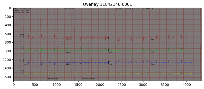
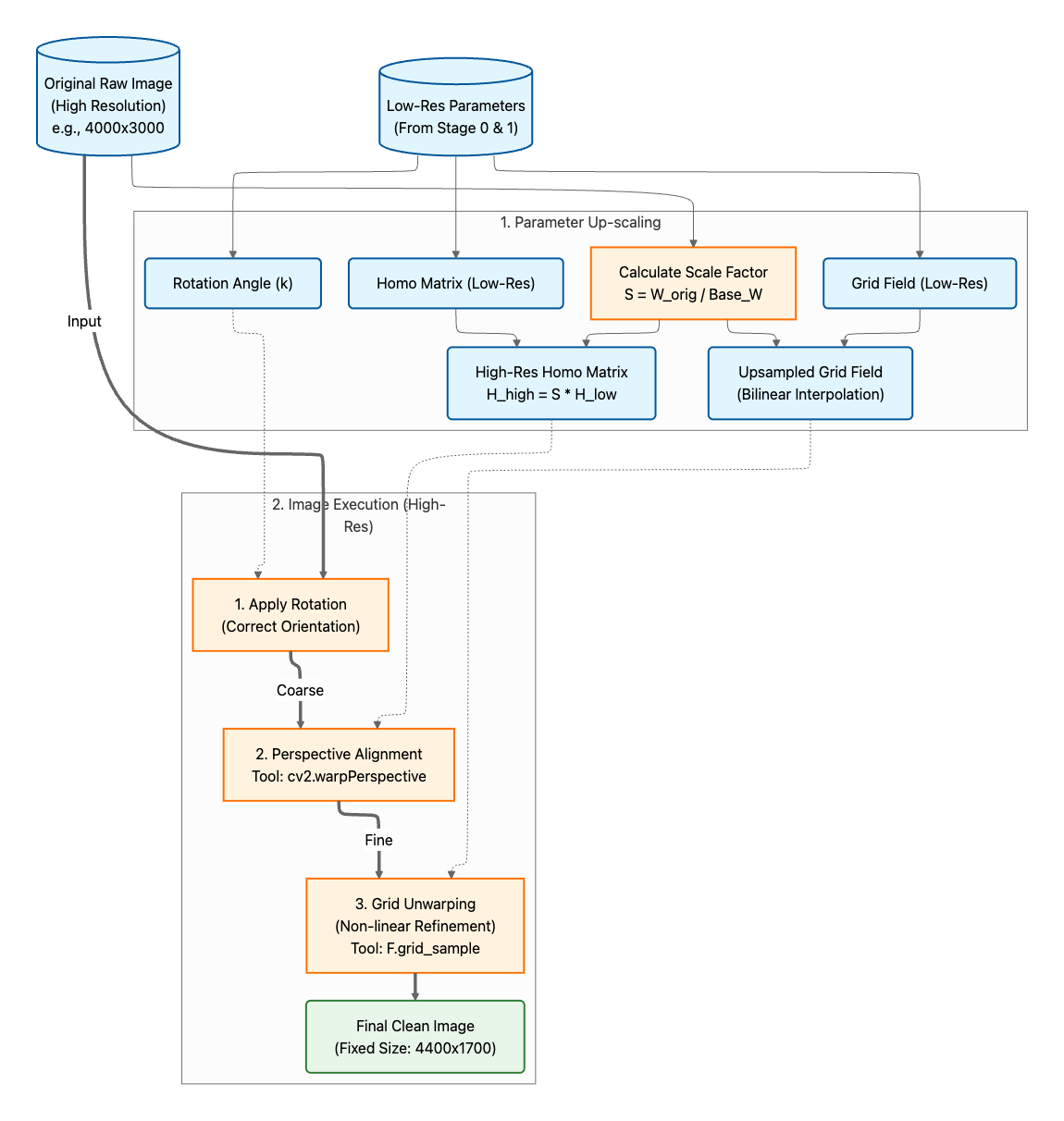
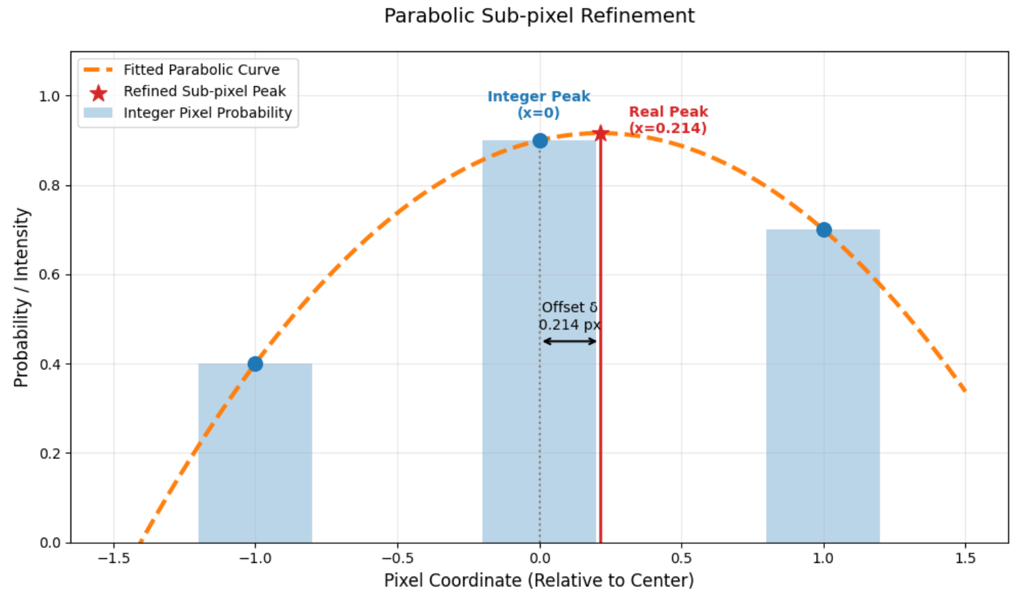
  "content": "<p>Thanks to PhysioNet and Kaggle for organizing this competition. Special thanks to <a href=\"https://www.kaggle.com/hengck23\" target=\"_blank\">@hengck23</a> for sharing the image rectification pipeline.</p>\n<h3>Overview</h3>\n<ul>\n<li><strong>High-Resolution Mapping Rectification:</strong> Calculate geometric parameters using low-resolution images, then scale them up and apply them directly to the original high-resolution images. This helps avoid losing details.</li>\n<li><strong>Training:</strong> Use strong data augmentation to make the model more robust.</li>\n<li><strong>Sub-pixel Precision:</strong> A parabolic refinement method is used to turn pixel-level predictions into accurate floating-point values.</li>\n</ul>\n<p>For full implementation details and source code, please refer to our GitHub repository and notebook:</p>\n<ul>\n<li>Training Code (GitHub): <a href=\"https://github.com/tanghaozhe/physionet-ecg-image-digitization-3rd-place\" target=\"_blank\">https://github.com/tanghaozhe/physionet-ecg-image-digitization-3rd-place</a></li>\n<li>Submition notebook: <a href=\"https://www.kaggle.com/code/hirotetsu/physionet-submission-3rd-place\" target=\"_blank\">https://www.kaggle.com/code/hirotetsu/physionet-submission-3rd-place</a></li>\n</ul>\n<h3>Mask Preparation</h3>\n<p>For mask generation, we draw a one-pixel-wide line using the signal data. We also tried making the line wider by adding a Gaussian blur to create softer labels, but this did not improve the results. Therefore, we decided to keep the one-pixel mask and intentionally trained an “overfitted” model so that it predicts thin waveforms with high confidence.</p>\n<table>\n<thead>\n<tr>\n<th>Image Size</th>\n<th>SNR (dB)</th>\n<th>Notes</th>\n</tr>\n</thead>\n<tbody>\n<tr>\n<td>2200 x 1700</td>\n<td>24.2235</td>\n<td>Standard dimension (200 DPI)</td>\n</tr>\n<tr>\n<td>4400 x 1700</td>\n<td>31.2271</td>\n<td>Selected dimension</td>\n</tr>\n</tbody>\n</table>\n<p><img src=\"https://www.googleapis.com/download/storage/v1/b/kaggle-user-content/o/inbox%2F2312281%2F9417a06baf76cb5a205ad8b20daa7d43%2Fkaggle_mask.png?generation=1769185919690734&amp;alt=media\" alt=\"\"></p>\n<ol>\n<li><p><strong>Wider Images:</strong>\nIncreasing the width to 4400 pixels greatly improves SNR. ECG signals are time-series data, so more horizontal pixels mean better sampling and less quantization error.</p></li>\n<li><p><strong>Fixed Height:</strong> \nThe height is kept the same. Keeping the waveform thickness close to 1 pixel helps the model predict the signal position more accurately and makes post-processing more stable.</p></li>\n</ol>\n<p>We evaluated SNR for different mask sizes and found that larger masks usually give better SNR. However, due to limited inference memory and training results, we chose to double the width while keeping the original height. the problem here, is how can we keep the quality of images in the rectification process, which we addressed by separating the image transformation step from the rectification process.</p>\n<h3>High-Resolution Mapping Rectification</h3>\n<p>The rectification model output relatively small size rectified images, which can cause quality loss during the rectification process. To avoid degradation caused by repeated resizing, we split the process into two steps:</p>\n<ul>\n<li>Parameter estimation (low resolution)</li>\n<li>Image transformation (high resolution)\n<img src=\"https://www.googleapis.com/download/storage/v1/b/kaggle-user-content/o/inbox%2F2312281%2Fe3df4813f6c4d98f023736424fe96e5a%2Fkaggle_map.png?generation=1769186108659597&amp;alt=media\" alt=\"\"></li>\n</ul>\n<p>The homography matrix and grid coordinates are scaled to match the size of the original raw image. This approach resulted in a significant improvement in the experiments</p>\n<h3>Signal Segmentation Model</h3>\n<ul>\n<li><p><strong>encoder:</strong></p>\n<ul>\n<li>ConvNeXt V2</li>\n<li>HRNet</li>\n<li>EfficientNet V2</li></ul>\n<p>In our experiments, the performance ranking was ConvNeXt V2 &gt; HRNet &gt; EfficientNet V2. For the final submission, we ensembled the ConvNeXt V2 and HRNet models by taking a weighted average of the post-processed signals, which will be introduced later, instead of directly averaging the segmentation probabilities. This signal-level ensembling produced better results.</p></li>\n<li><p><strong>decoder:</strong></p>\n<ul>\n<li>UnetDecoder</li></ul></li>\n<li><p><strong>Augmentation:</strong></p>\n<ul>\n<li>GridDropout</li>\n<li>CoarseDropout</li>\n<li>AddPerlinDirt</li>\n<li>MotionBlur</li>\n<li>Downscale</li>\n<li>GaussianBlur</li>\n<li>ImageCompression</li>\n<li>GaussNoise</li>\n<li>ISONoise</li>\n<li>ToGray</li>\n<li>RandomBrightnessContrast</li>\n<li>HueSaturationValue</li>\n<li>RandomShadow</li>\n<li>ElasticTransform</li>\n<li>HorizontalFlip</li>\n<li>VerticalFlip</li></ul>\n<p>Considering that some samples in the hidden test data may be highly noisy, we applied very aggressive data augmentation during training. We added a small ElasticTransform to simulate distortions in the unwrapped images, where both the waveforms and grid lines may be slightly warped by the unwrapping process itself.</p></li>\n<li><p><strong>Loss:</strong>\nWe trained the model using BCE loss. In practice, even at the lowest loss, the predicted waveforms were still too thick. To obtain thin, nearly one-pixel-wide waveform boundaries, we deliberately continued training an “overfitted” model and used the Dice score and CV score as the main criteria for model selection.</p></li>\n</ul>\n<h3>Sub-pixel Signal Processing</h3>\n<p>We experimented with different strategies to convert pixel locations into time-series values. Two effective approaches are:</p>\n<ul>\n<li>Weighted Centroid：We selected the top-𝐾 pixels and computed the final position using the predicted probabilities as weights. This approach produced good results, but it is sensitive to the choice of 𝐾 and the weighting exponent.</li>\n<li>Parabolic Interpolation: It refines the integer argmax by fitting a local parabola to the peak and its two neighbors, giving a sub-pixel (floating-point) peak position.</li>\n</ul>\n<p>We chose parabolic interpolation because it consistently delivered the best performance in our experiments. We believe this is because the model outputs very thin, sharp lines, for which parabolic interpolation provides a reliable way to estimate the true position without requiring hyperparameter tuning.</p>\n<p><img src=\"https://www.googleapis.com/download/storage/v1/b/kaggle-user-content/o/inbox%2F2312281%2Fb02f84fd0ba22396484907126cc1e285%2Fkaggle_pixel.png?generation=1769186198184631&amp;alt=media\" alt=\"\"></p>\n<p>The offset is computed as:</p>\n<p>delta = (y_left - y_right) / (2 * (y_left - 2*y_center + y_right))</p>\n<p>The final position is:</p>\n<p>Real Coordinate = Integer Index + delta</p>\n<h3>Others</h3>\n<ul>\n<li><strong>Lead II Fusion:</strong> Merges the short Lead II prediction with the long rhythm strip (Series 3) by averaging the overlapping head region.</li>\n<li><strong>Einthoven Correction:</strong> Applies Einthoven Correction to adjust Leads I, II, and III while enforcing the physical constraint II=I+III. Lead II is given higher importance (weight = 2), while Leads I and III use equal lower weights (weight = 1).</li>\n<li><strong>TTA:</strong> original, horizontal flip, vertical flip, and both flips</li>\n</ul>",
  "messages": [
    {
      "id": "3395783",
      "postDate": "01/23/2026 16:43:19",
      "content": "<p>Thanks to PhysioNet and Kaggle for organizing this competition. Special thanks to <a href=\"https://www.kaggle.com/hengck23\" target=\"_blank\">@hengck23</a> for sharing the image rectification pipeline.</p>\n<h3>Overview</h3>\n<ul>\n<li><strong>High-Resolution Mapping Rectification:</strong> Calculate geometric parameters using low-resolution images, then scale them up and apply them directly to the original high-resolution images. This helps avoid losing details.</li>\n<li><strong>Training:</strong> Use strong data augmentation to make the model more robust.</li>\n<li><strong>Sub-pixel Precision:</strong> A parabolic refinement method is used to turn pixel-level predictions into accurate floating-point values.</li>\n</ul>\n<p>For full implementation details and source code, please refer to our GitHub repository and notebook:</p>\n<ul>\n<li>Training Code (GitHub): <a href=\"https://github.com/tanghaozhe/physionet-ecg-image-digitization-3rd-place\" target=\"_blank\">https://github.com/tanghaozhe/physionet-ecg-image-digitization-3rd-place</a></li>\n<li>Submition notebook: <a href=\"https://www.kaggle.com/code/hirotetsu/physionet-submission-3rd-place\" target=\"_blank\">https://www.kaggle.com/code/hirotetsu/physionet-submission-3rd-place</a></li>\n</ul>\n<h3>Mask Preparation</h3>\n<p>For mask generation, we draw a one-pixel-wide line using the signal data. We also tried making the line wider by adding a Gaussian blur to create softer labels, but this did not improve the results. Therefore, we decided to keep the one-pixel mask and intentionally trained an “overfitted” model so that it predicts thin waveforms with high confidence.</p>\n<table>\n<thead>\n<tr>\n<th>Image Size</th>\n<th>SNR (dB)</th>\n<th>Notes</th>\n</tr>\n</thead>\n<tbody>\n<tr>\n<td>2200 x 1700</td>\n<td>24.2235</td>\n<td>Standard dimension (200 DPI)</td>\n</tr>\n<tr>\n<td>4400 x 1700</td>\n<td>31.2271</td>\n<td>Selected dimension</td>\n</tr>\n</tbody>\n</table>\n<p><img src=\"https://www.googleapis.com/download/storage/v1/b/kaggle-user-content/o/inbox%2F2312281%2F9417a06baf76cb5a205ad8b20daa7d43%2Fkaggle_mask.png?generation=1769185919690734&amp;alt=media\" alt=\"\"></p>\n<ol>\n<li><p><strong>Wider Images:</strong>\nIncreasing the width to 4400 pixels greatly improves SNR. ECG signals are time-series data, so more horizontal pixels mean better sampling and less quantization error.</p></li>\n<li><p><strong>Fixed Height:</strong> \nThe height is kept the same. Keeping the waveform thickness close to 1 pixel helps the model predict the signal position more accurately and makes post-processing more stable.</p></li>\n</ol>\n<p>We evaluated SNR for different mask sizes and found that larger masks usually give better SNR. However, due to limited inference memory and training results, we chose to double the width while keeping the original height. the problem here, is how can we keep the quality of images in the rectification process, which we addressed by separating the image transformation step from the rectification process.</p>\n<h3>High-Resolution Mapping Rectification</h3>\n<p>The rectification model output relatively small size rectified images, which can cause quality loss during the rectification process. To avoid degradation caused by repeated resizing, we split the process into two steps:</p>\n<ul>\n<li>Parameter estimation (low resolution)</li>\n<li>Image transformation (high resolution)\n<img src=\"https://www.googleapis.com/download/storage/v1/b/kaggle-user-content/o/inbox%2F2312281%2Fe3df4813f6c4d98f023736424fe96e5a%2Fkaggle_map.png?generation=1769186108659597&amp;alt=media\" alt=\"\"></li>\n</ul>\n<p>The homography matrix and grid coordinates are scaled to match the size of the original raw image. This approach resulted in a significant improvement in the experiments</p>\n<h3>Signal Segmentation Model</h3>\n<ul>\n<li><p><strong>encoder:</strong></p>\n<ul>\n<li>ConvNeXt V2</li>\n<li>HRNet</li>\n<li>EfficientNet V2</li></ul>\n<p>In our experiments, the performance ranking was ConvNeXt V2 &gt; HRNet &gt; EfficientNet V2. For the final submission, we ensembled the ConvNeXt V2 and HRNet models by taking a weighted average of the post-processed signals, which will be introduced later, instead of directly averaging the segmentation probabilities. This signal-level ensembling produced better results.</p></li>\n<li><p><strong>decoder:</strong></p>\n<ul>\n<li>UnetDecoder</li></ul></li>\n<li><p><strong>Augmentation:</strong></p>\n<ul>\n<li>GridDropout</li>\n<li>CoarseDropout</li>\n<li>AddPerlinDirt</li>\n<li>MotionBlur</li>\n<li>Downscale</li>\n<li>GaussianBlur</li>\n<li>ImageCompression</li>\n<li>GaussNoise</li>\n<li>ISONoise</li>\n<li>ToGray</li>\n<li>RandomBrightnessContrast</li>\n<li>HueSaturationValue</li>\n<li>RandomShadow</li>\n<li>ElasticTransform</li>\n<li>HorizontalFlip</li>\n<li>VerticalFlip</li></ul>\n<p>Considering that some samples in the hidden test data may be highly noisy, we applied very aggressive data augmentation during training. We added a small ElasticTransform to simulate distortions in the unwrapped images, where both the waveforms and grid lines may be slightly warped by the unwrapping process itself.</p></li>\n<li><p><strong>Loss:</strong>\nWe trained the model using BCE loss. In practice, even at the lowest loss, the predicted waveforms were still too thick. To obtain thin, nearly one-pixel-wide waveform boundaries, we deliberately continued training an “overfitted” model and used the Dice score and CV score as the main criteria for model selection.</p></li>\n</ul>\n<h3>Sub-pixel Signal Processing</h3>\n<p>We experimented with different strategies to convert pixel locations into time-series values. Two effective approaches are:</p>\n<ul>\n<li>Weighted Centroid：We selected the top-𝐾 pixels and computed the final position using the predicted probabilities as weights. This approach produced good results, but it is sensitive to the choice of 𝐾 and the weighting exponent.</li>\n<li>Parabolic Interpolation: It refines the integer argmax by fitting a local parabola to the peak and its two neighbors, giving a sub-pixel (floating-point) peak position.</li>\n</ul>\n<p>We chose parabolic interpolation because it consistently delivered the best performance in our experiments. We believe this is because the model outputs very thin, sharp lines, for which parabolic interpolation provides a reliable way to estimate the true position without requiring hyperparameter tuning.</p>\n<p><img src=\"https://www.googleapis.com/download/storage/v1/b/kaggle-user-content/o/inbox%2F2312281%2Fb02f84fd0ba22396484907126cc1e285%2Fkaggle_pixel.png?generation=1769186198184631&amp;alt=media\" alt=\"\"></p>\n<p>The offset is computed as:</p>\n<p>delta = (y_left - y_right) / (2 * (y_left - 2*y_center + y_right))</p>\n<p>The final position is:</p>\n<p>Real Coordinate = Integer Index + delta</p>\n<h3>Others</h3>\n<ul>\n<li><strong>Lead II Fusion:</strong> Merges the short Lead II prediction with the long rhythm strip (Series 3) by averaging the overlapping head region.</li>\n<li><strong>Einthoven Correction:</strong> Applies Einthoven Correction to adjust Leads I, II, and III while enforcing the physical constraint II=I+III. Lead II is given higher importance (weight = 2), while Leads I and III use equal lower weights (weight = 1).</li>\n<li><strong>TTA:</strong> original, horizontal flip, vertical flip, and both flips</li>\n</ul>",
      "rawMarkdown": "Thanks to PhysioNet and Kaggle for organizing this competition. Special thanks to @hengck23 for sharing the image rectification pipeline.\n\n### Overview\n\n- **High-Resolution Mapping Rectification:** Calculate geometric parameters using low-resolution images, then scale them up and apply them directly to the original high-resolution images. This helps avoid losing details.\n- **Training:** Use strong data augmentation to make the model more robust.\n- **Sub-pixel Precision:** A parabolic refinement method is used to turn pixel-level predictions into accurate floating-point values.\n\nFor full implementation details and source code, please refer to our GitHub repository and notebook:\n- Training Code (GitHub): https://github.com/tanghaozhe/physionet-ecg-image-digitization-3rd-place\n- Submition notebook: https://www.kaggle.com/code/hirotetsu/physionet-submission-3rd-place\n\n\n### Mask Preparation\nFor mask generation, we draw a one-pixel-wide line using the signal data. We also tried making the line wider by adding a Gaussian blur to create softer labels, but this did not improve the results. Therefore, we decided to keep the one-pixel mask and intentionally trained an “overfitted” model so that it predicts thin waveforms with high confidence.\n\n| Image Size |SNR (dB)  | Notes|\n| --- | --- |\n| 2200 x 1700 | 24.2235 | Standard dimension (200 DPI) |\n| 4400 x 1700 | 31.2271 | Selected dimension |\n\n![](https://www.googleapis.com/download/storage/v1/b/kaggle-user-content/o/inbox%2F2312281%2F9417a06baf76cb5a205ad8b20daa7d43%2Fkaggle_mask.png?generation=1769185919690734&alt=media)\n\n1. **Wider Images:**\nIncreasing the width to 4400 pixels greatly improves SNR. ECG signals are time-series data, so more horizontal pixels mean better sampling and less quantization error.\n    \n2. **Fixed Height:** \nThe height is kept the same. Keeping the waveform thickness close to 1 pixel helps the model predict the signal position more accurately and makes post-processing more stable.\n\nWe evaluated SNR for different mask sizes and found that larger masks usually give better SNR. However, due to limited inference memory and training results, we chose to double the width while keeping the original height. the problem here, is how can we keep the quality of images in the rectification process, which we addressed by separating the image transformation step from the rectification process.\n\n### High-Resolution Mapping Rectification\nThe rectification model output relatively small size rectified images, which can cause quality loss during the rectification process. To avoid degradation caused by repeated resizing, we split the process into two steps:\n- Parameter estimation (low resolution)\n- Image transformation (high resolution)\n![](https://www.googleapis.com/download/storage/v1/b/kaggle-user-content/o/inbox%2F2312281%2Fe3df4813f6c4d98f023736424fe96e5a%2Fkaggle_map.png?generation=1769186108659597&alt=media)\n\nThe homography matrix and grid coordinates are scaled to match the size of the original raw image. This approach resulted in a significant improvement in the experiments\n\n### Signal Segmentation Model\n- **encoder:**\n    - ConvNeXt V2\n    - HRNet\n    - EfficientNet V2\n\n    In our experiments, the performance ranking was ConvNeXt V2 > HRNet > EfficientNet V2. For the final submission, we ensembled the ConvNeXt V2 and HRNet models by taking a weighted average of the post-processed signals, which will be introduced later, instead of directly averaging the segmentation probabilities. This signal-level ensembling produced better results.\n\n- **decoder:**\n    - UnetDecoder\n\n- **Augmentation:**\n    - GridDropout\n    - CoarseDropout\n    - AddPerlinDirt\n    - MotionBlur\n    - Downscale\n    - GaussianBlur\n    - ImageCompression\n    - GaussNoise\n    - ISONoise\n    - ToGray\n    - RandomBrightnessContrast\n    - HueSaturationValue\n    - RandomShadow\n    - ElasticTransform\n    - HorizontalFlip\n    - VerticalFlip\n\n    Considering that some samples in the hidden test data may be highly noisy, we applied very aggressive data augmentation during training. We added a small ElasticTransform to simulate distortions in the unwrapped images, where both the waveforms and grid lines may be slightly warped by the unwrapping process itself.\n\n- **Loss:**\nWe trained the model using BCE loss. In practice, even at the lowest loss, the predicted waveforms were still too thick. To obtain thin, nearly one-pixel-wide waveform boundaries, we deliberately continued training an “overfitted” model and used the Dice score and CV score as the main criteria for model selection.\n\n### Sub-pixel Signal Processing\n\nWe experimented with different strategies to convert pixel locations into time-series values. Two effective approaches are:\n- Weighted Centroid：We selected the top-𝐾 pixels and computed the final position using the predicted probabilities as weights. This approach produced good results, but it is sensitive to the choice of 𝐾 and the weighting exponent.\n- Parabolic Interpolation: It refines the integer argmax by fitting a local parabola to the peak and its two neighbors, giving a sub-pixel (floating-point) peak position.\n\nWe chose parabolic interpolation because it consistently delivered the best performance in our experiments. We believe this is because the model outputs very thin, sharp lines, for which parabolic interpolation provides a reliable way to estimate the true position without requiring hyperparameter tuning.\n\n![](https://www.googleapis.com/download/storage/v1/b/kaggle-user-content/o/inbox%2F2312281%2Fb02f84fd0ba22396484907126cc1e285%2Fkaggle_pixel.png?generation=1769186198184631&alt=media)\n\nThe offset is computed as:\n\ndelta = (y_left - y_right) / (2 * (y_left - 2*y_center + y_right))\n\nThe final position is:\n\nReal Coordinate = Integer Index + delta\n\n### Others\n- **Lead II Fusion:** Merges the short Lead II prediction with the long rhythm strip (Series 3) by averaging the overlapping head region.\n- **Einthoven Correction:** Applies Einthoven Correction to adjust Leads I, II, and III while enforcing the physical constraint II=I+III. Lead II is given higher importance (weight = 2), while Leads I and III use equal lower weights (weight = 1).\n- **TTA:** original, horizontal flip, vertical flip, and both flips",
      "votes": null
    },
    {
      "id": "3396095",
      "postDate": "01/24/2026 09:57:18",
      "content": "<p>Congratulations! thanks for sharing. How did you get mask GT?  Did you train segmentation model by using rectified images of all types for each case_id? if yes , did you rectify the mask like for the images?</p>",
      "rawMarkdown": "Congratulations! thanks for sharing. How did you get mask GT?  Did you train segmentation model by using rectified images of all types for each case_id? if yes , did you rectify the mask like for the images?",
      "votes": null
    },
    {
      "id": "3396606",
      "postDate": "01/25/2026 12:16:30",
      "content": "<p>Thanks for reading. I plot a one-pixel-wide line on the mask. I use the same mask for all images with the same ID.</p>",
      "rawMarkdown": "Thanks for reading. I plot a one-pixel-wide line on the mask. I use the same mask for all images with the same ID.",
      "votes": null
    }
  ],
  "comments": [
    {
      "id": 3396095,
      "author_name": "vandongtran",
      "author_url": "",
      "post_date": "01/24/2026 09:57:18",
      "content": "<p>Congratulations! thanks for sharing. How did you get mask GT?  Did you train segmentation model by using rectified images of all types for each case_id? if yes , did you rectify the mask like for the images?</p>",
      "votes": null,
      "replies": [
        {
          "id": 3396606,
          "author_name": "hirotetsu",
          "author_url": "",
          "post_date": "01/25/2026 12:16:30",
          "content": "<p>Thanks for reading. I plot a one-pixel-wide line on the mask. I use the same mask for all images with the same ID.</p>",
          "votes": null,
          "replies": []
        }
      ]
    }
  ],
  "raw_markdown_by_id": {
    "3395783": "Thanks to PhysioNet and Kaggle for organizing this competition. Special thanks to @hengck23 for sharing the image rectification pipeline.\n\n### Overview\n\n- **High-Resolution Mapping Rectification:** Calculate geometric parameters using low-resolution images, then scale them up and apply them directly to the original high-resolution images. This helps avoid losing details.\n- **Training:** Use strong data augmentation to make the model more robust.\n- **Sub-pixel Precision:** A parabolic refinement method is used to turn pixel-level predictions into accurate floating-point values.\n\nFor full implementation details and source code, please refer to our GitHub repository and notebook:\n- Training Code (GitHub): https://github.com/tanghaozhe/physionet-ecg-image-digitization-3rd-place\n- Submition notebook: https://www.kaggle.com/code/hirotetsu/physionet-submission-3rd-place\n\n\n### Mask Preparation\nFor mask generation, we draw a one-pixel-wide line using the signal data. We also tried making the line wider by adding a Gaussian blur to create softer labels, but this did not improve the results. Therefore, we decided to keep the one-pixel mask and intentionally trained an “overfitted” model so that it predicts thin waveforms with high confidence.\n\n| Image Size |SNR (dB)  | Notes|\n| --- | --- |\n| 2200 x 1700 | 24.2235 | Standard dimension (200 DPI) |\n| 4400 x 1700 | 31.2271 | Selected dimension |\n\n![](https://www.googleapis.com/download/storage/v1/b/kaggle-user-content/o/inbox%2F2312281%2F9417a06baf76cb5a205ad8b20daa7d43%2Fkaggle_mask.png?generation=1769185919690734&alt=media)\n\n1. **Wider Images:**\nIncreasing the width to 4400 pixels greatly improves SNR. ECG signals are time-series data, so more horizontal pixels mean better sampling and less quantization error.\n    \n2. **Fixed Height:** \nThe height is kept the same. Keeping the waveform thickness close to 1 pixel helps the model predict the signal position more accurately and makes post-processing more stable.\n\nWe evaluated SNR for different mask sizes and found that larger masks usually give better SNR. However, due to limited inference memory and training results, we chose to double the width while keeping the original height. the problem here, is how can we keep the quality of images in the rectification process, which we addressed by separating the image transformation step from the rectification process.\n\n### High-Resolution Mapping Rectification\nThe rectification model output relatively small size rectified images, which can cause quality loss during the rectification process. To avoid degradation caused by repeated resizing, we split the process into two steps:\n- Parameter estimation (low resolution)\n- Image transformation (high resolution)\n![](https://www.googleapis.com/download/storage/v1/b/kaggle-user-content/o/inbox%2F2312281%2Fe3df4813f6c4d98f023736424fe96e5a%2Fkaggle_map.png?generation=1769186108659597&alt=media)\n\nThe homography matrix and grid coordinates are scaled to match the size of the original raw image. This approach resulted in a significant improvement in the experiments\n\n### Signal Segmentation Model\n- **encoder:**\n    - ConvNeXt V2\n    - HRNet\n    - EfficientNet V2\n\n    In our experiments, the performance ranking was ConvNeXt V2 > HRNet > EfficientNet V2. For the final submission, we ensembled the ConvNeXt V2 and HRNet models by taking a weighted average of the post-processed signals, which will be introduced later, instead of directly averaging the segmentation probabilities. This signal-level ensembling produced better results.\n\n- **decoder:**\n    - UnetDecoder\n\n- **Augmentation:**\n    - GridDropout\n    - CoarseDropout\n    - AddPerlinDirt\n    - MotionBlur\n    - Downscale\n    - GaussianBlur\n    - ImageCompression\n    - GaussNoise\n    - ISONoise\n    - ToGray\n    - RandomBrightnessContrast\n    - HueSaturationValue\n    - RandomShadow\n    - ElasticTransform\n    - HorizontalFlip\n    - VerticalFlip\n\n    Considering that some samples in the hidden test data may be highly noisy, we applied very aggressive data augmentation during training. We added a small ElasticTransform to simulate distortions in the unwrapped images, where both the waveforms and grid lines may be slightly warped by the unwrapping process itself.\n\n- **Loss:**\nWe trained the model using BCE loss. In practice, even at the lowest loss, the predicted waveforms were still too thick. To obtain thin, nearly one-pixel-wide waveform boundaries, we deliberately continued training an “overfitted” model and used the Dice score and CV score as the main criteria for model selection.\n\n### Sub-pixel Signal Processing\n\nWe experimented with different strategies to convert pixel locations into time-series values. Two effective approaches are:\n- Weighted Centroid：We selected the top-𝐾 pixels and computed the final position using the predicted probabilities as weights. This approach produced good results, but it is sensitive to the choice of 𝐾 and the weighting exponent.\n- Parabolic Interpolation: It refines the integer argmax by fitting a local parabola to the peak and its two neighbors, giving a sub-pixel (floating-point) peak position.\n\nWe chose parabolic interpolation because it consistently delivered the best performance in our experiments. We believe this is because the model outputs very thin, sharp lines, for which parabolic interpolation provides a reliable way to estimate the true position without requiring hyperparameter tuning.\n\n![](https://www.googleapis.com/download/storage/v1/b/kaggle-user-content/o/inbox%2F2312281%2Fb02f84fd0ba22396484907126cc1e285%2Fkaggle_pixel.png?generation=1769186198184631&alt=media)\n\nThe offset is computed as:\n\ndelta = (y_left - y_right) / (2 * (y_left - 2*y_center + y_right))\n\nThe final position is:\n\nReal Coordinate = Integer Index + delta\n\n### Others\n- **Lead II Fusion:** Merges the short Lead II prediction with the long rhythm strip (Series 3) by averaging the overlapping head region.\n- **Einthoven Correction:** Applies Einthoven Correction to adjust Leads I, II, and III while enforcing the physical constraint II=I+III. Lead II is given higher importance (weight = 2), while Leads I and III use equal lower weights (weight = 1).\n- **TTA:** original, horizontal flip, vertical flip, and both flips",
    "3396095": "Congratulations! thanks for sharing. How did you get mask GT?  Did you train segmentation model by using rectified images of all types for each case_id? if yes , did you rectify the mask like for the images?",
    "3396606": "Thanks for reading. I plot a one-pixel-wide line on the mask. I use the same mask for all images with the same ID."
  },
  "source": "meta"
}