
Thank you to PhysioNet, the competition host, Kaggle, and everyone else involved for putting together such a challenging and interesting competition. Before entering this competition, I probably would have laughed off even the idea of doing this as magic so it is very gratifying to come away understanding a practical application of computer vision that I didn't realize was possible.
\nSpecial thanks to @hengck23 and also @kami1976 whose notebooks provided the initial starting point of my solution. Also thank you to whoever came up with the algorithm for Einthoven error correction which I apply to my signals at the very end, @antonoof maybe?
\nAs suggested by my subtitle, my solution is for the most part an extension of hengck23's original demo submission notebook, although I do provide some significant changes. The following sections describe the basic flow of my inference pipeline.
\n
Stage A - Orientation
\nIn the first stage of my pipeline I call the first part of @hengck23's stage0's model to get a properly oriented image and the location of its key point markers.
\nStage B - Homography
\n@hengck23's stage0 uses homography to warp and output a canonical image at 1440x1152 resolution which is significantly lower than the 2200x1700 ecg images generated by ecg-image-kit. In Stage B, I create both that lower resolution image as well as a high resolution 2400x1920 image designed to preserve as much information as possible from the original ECG.
\nStage C - Rectification
\nStage C consists of the following main steps:
\nStage D - Signal Extraction
\nI follow essentially the same process as in the demo submission notebook with the following exceptions:
\nStage E - Post Processing
\nFor post processing I do two things:
\nGrid Point Refinement
\nThe grid point detection in the demo submission notebook is good, but not perfect. If you look closely at the image on the left you can see small deformations in the ECG grid where the grid point detection is off by a pixel or two. These deformations, of course, directly impact signal accuracy so getting them as accurate as possible helps SNR. As mentioned above, I used the @hengck23's stage1 network to initially predict the image gridpoints, then I passed each gridpoint through a cascade of two refinement networks to locate each as accurately as possible. The image on the right shows the resulting grid which is nearly perfect.
\n| Before | \nAfter | \n
 | \n  | \n
Below are the refined grid points in green plotted on top of the slightly larger radius original predictions in red. If you imagine pushing the red predictions into the green, you can see how the deformations in the image to the left occurred.
\n
To refine the grid points i trained 2 x 5 layer heatmap based CNNs each utilizing a 31x31 input patch and dilations to ensure the receptive field covered the entire patch. The first network was trained with 5 pixel vertical and horizontal translation (among other augmentations) whereas the second was trained with only 2 pixel translation. The initial grid point predictions where passed to the first network, and it's predictions were passed to the second. Because the second network was trained with a simpler problem to solve, it achieved better accuracy than the first at the expense of the deviations it was able to tolerate in it's input. If you believe the final validation error for second network, the average euclidean distance between the predicted location and the labels was only 0.146 pixels.
\n
Hand labeling
\nI pre-trained the refinement grids with the original grid point predictions and then fine tuned each with a set of 800 hand-labeled locations for training, 100 per non-0001 image type, and 180 for validation. For type 0001, I randomly selected grid point locations from the entire set of images. I initially used labelme to do the hand labeling, but ultimately built a custom labeler that would show the position of the original prediction for reference.
\n
Soft Labels
\nInstead of using hard labels where a pixel is set to either 0 or 1, I used soft labels such that the intensity of the two adjacent pixels between which the signal passes is set related to how close the signal is to the center of each. For instance if the signal is 0.1 pixels distant from the first pixel's center, it gets a value of 0.9 whereas the adjacent pixel gets a value of 0.1. The value of soft labels over hard labels in this case is it allows the labels to be specified at sub-pixel resolution. The following image shows hard and soft labels.
\n
Dual Mode Training
\nFor Stage D, I used essentially the same model as the original stage2 model with the exception that whereas the original model adds the y coordinates of the image into the final layer of the network, I add both the x and y coordinates. This makes it a challenge to do spatial augmentations, such as rotations or perspective shifts as both make it difficult to set the x and y coordinates properly. To get around this, during training I trained the network both before and after the final layer with 0.5 probability. When training before the final layer, I would do the more problematic rotation and perspective shift augmentations. When training after the final layer, I would only do augmentations, such as horizontal translation and color shifts.
", "messages": [ { "id": "3395696", "postDate": "01/23/2026 14:01:40", "content": "Thank you to PhysioNet, the competition host, Kaggle, and everyone else involved for putting together such a challenging and interesting competition. Before entering this competition, I probably would have laughed off even the idea of doing this as magic so it is very gratifying to come away understanding a practical application of computer vision that I didn't realize was possible.
\nSpecial thanks to @hengck23 and also @kami1976 whose notebooks provided the initial starting point of my solution. Also thank you to whoever came up with the algorithm for Einthoven error correction which I apply to my signals at the very end, @antonoof maybe?
\nAs suggested by my subtitle, my solution is for the most part an extension of hengck23's original demo submission notebook, although I do provide some significant changes. The following sections describe the basic flow of my inference pipeline.
\n
Stage A - Orientation
\nIn the first stage of my pipeline I call the first part of @hengck23's stage0's model to get a properly oriented image and the location of its key point markers.
\nStage B - Homography
\n@hengck23's stage0 uses homography to warp and output a canonical image at 1440x1152 resolution which is significantly lower than the 2200x1700 ecg images generated by ecg-image-kit. In Stage B, I create both that lower resolution image as well as a high resolution 2400x1920 image designed to preserve as much information as possible from the original ECG.
\nStage C - Rectification
\nStage C consists of the following main steps:
\nStage D - Signal Extraction
\nI follow essentially the same process as in the demo submission notebook with the following exceptions:
\nStage E - Post Processing
\nFor post processing I do two things:
\nGrid Point Refinement
\nThe grid point detection in the demo submission notebook is good, but not perfect. If you look closely at the image on the left you can see small deformations in the ECG grid where the grid point detection is off by a pixel or two. These deformations, of course, directly impact signal accuracy so getting them as accurate as possible helps SNR. As mentioned above, I used the @hengck23's stage1 network to initially predict the image gridpoints, then I passed each gridpoint through a cascade of two refinement networks to locate each as accurately as possible. The image on the right shows the resulting grid which is nearly perfect.
\n| Before | \nAfter | \n
| \n | \n
Below are the refined grid points in green plotted on top of the slightly larger radius original predictions in red. If you imagine pushing the red predictions into the green, you can see how the deformations in the image to the left occurred.
\n
To refine the grid points i trained 2 x 5 layer heatmap based CNNs each utilizing a 31x31 input patch and dilations to ensure the receptive field covered the entire patch. The first network was trained with 5 pixel vertical and horizontal translation (among other augmentations) whereas the second was trained with only 2 pixel translation. The initial grid point predictions where passed to the first network, and it's predictions were passed to the second. Because the second network was trained with a simpler problem to solve, it achieved better accuracy than the first at the expense of the deviations it was able to tolerate in it's input. If you believe the final validation error for second network, the average euclidean distance between the predicted location and the labels was only 0.146 pixels.
\n
Hand labeling
\nI pre-trained the refinement grids with the original grid point predictions and then fine tuned each with a set of 800 hand-labeled locations for training, 100 per non-0001 image type, and 180 for validation. For type 0001, I randomly selected grid point locations from the entire set of images. I initially used labelme to do the hand labeling, but ultimately built a custom labeler that would show the position of the original prediction for reference.
\n
Soft Labels
\nInstead of using hard labels where a pixel is set to either 0 or 1, I used soft labels such that the intensity of the two adjacent pixels between which the signal passes is set related to how close the signal is to the center of each. For instance if the signal is 0.1 pixels distant from the first pixel's center, it gets a value of 0.9 whereas the adjacent pixel gets a value of 0.1. The value of soft labels over hard labels in this case is it allows the labels to be specified at sub-pixel resolution. The following image shows hard and soft labels.
\n
Dual Mode Training
\nFor Stage D, I used essentially the same model as the original stage2 model with the exception that whereas the original model adds the y coordinates of the image into the final layer of the network, I add both the x and y coordinates. This makes it a challenge to do spatial augmentations, such as rotations or perspective shifts as both make it difficult to set the x and y coordinates properly. To get around this, during training I trained the network both before and after the final layer with 0.5 probability. When training before the final layer, I would do the more problematic rotation and perspective shift augmentations. When training after the final layer, I would only do augmentations, such as horizontal translation and color shifts.
", "rawMarkdown": "Thank you to PhysioNet, the competition host, Kaggle, and everyone else involved for putting together such a challenging and interesting competition. Before entering this competition, I probably would have laughed off even the idea of doing this as magic so it is very gratifying to come away understanding a practical application of computer vision that I didn't realize was possible.\n\nSpecial thanks to @hengck23 and also @kami1976 whose notebooks provided the initial starting point of my solution. Also thank you to whoever came up with the algorithm for Einthoven error correction which I apply to my signals at the very end, @antonoof maybe?\n\nAs suggested by my subtitle, my solution is for the most part an extension of hengck23's original [demo submission](https://www.kaggle.com/code/hengck23/demo-submission) notebook, although I do provide some significant changes. The following sections describe the basic flow of my inference pipeline.\n\n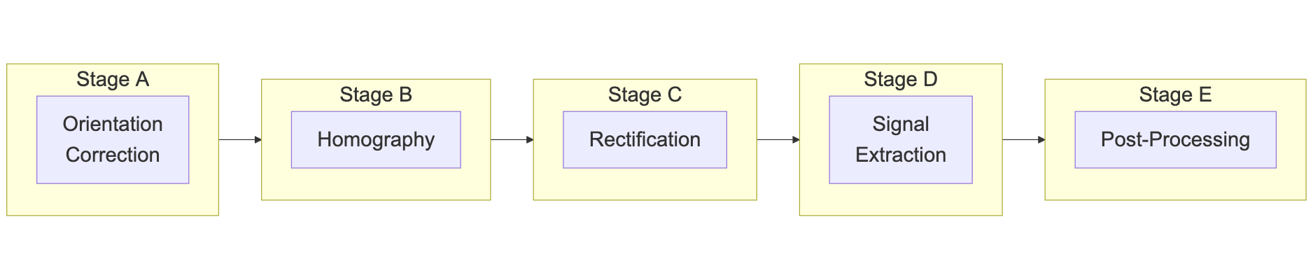\n\n**Stage A - Orientation**\n\nIn the first stage of my pipeline I call the first part of @hengck23's stage0's model to get a properly oriented image and the location of its key point markers.\n\n**Stage B - Homography**\n\n@hengck23's stage0 uses homography to warp and output a canonical image at 1440x1152 resolution which is significantly lower than the 2200x1700 ecg images generated by ecg-image-kit. In Stage B, I create both that lower resolution image as well as a high resolution 2400x1920 image designed to preserve as much information as possible from the original ECG.\n\n**Stage C - Rectification**\n\nStage C consists of the following main steps:\n- Pass the low resolution 1440x1152 image from Stage B through @hengck23's stage0 model to get the grid point locations.\n- Convert those low resolution grid points into the coordinate system of the high resolution 2400x1920 image.\n- Pass the high resolution grid points through a cascade of refinement neural networks to refine their positions to (hopefully) sub-pixel accuracy.\n- Perform rectification on the high resolution image with the refined grid points.\n\n**Stage D - Signal Extraction**\n\nI follow essentially the same process as in the [demo submission](https://www.kaggle.com/code/hengck23/demo-submission) notebook with the following exceptions:\n- Instead of performing it on the original image, I scale the image to twice it's length as recommended by @hengck23 in one of the [discussion posts.](https://www.kaggle.com/competitions/physionet-ecg-image-digitization/discussion/624054). Note, that I actually tried various resolutions, 2x2, 1x2, 1x4, and 1x8, but 1x2 pretty easily outperforms the others.\n- Because I use soft labels, I extract the signal using weighted averaging of a window around argmax. Surprisingly, a window of 100 pixels in each direction worked best with diminishing returns after that. Likely this does a better job of estimating the QRS spikes.\n- The image is processed in patches and passed through an ensemble of 10 models trained with different random seeds.\n\n**Stage E - Post Processing**\n\nFor post processing I do two things:\n- I ensemble the first 1/4 of the long II lead with the short II lead.\n- I use the Einthoven error correction algorithm found in several of the public notebooks.\n\n**Grid Point Refinement**\n\nThe grid point detection in the [demo submission notebook](https://www.kaggle.com/code/hengck23/demo-submission) is good, but not perfect. If you look closely at the image on the left you can see small deformations in the ECG grid where the grid point detection is off by a pixel or two. These deformations, of course, directly impact signal accuracy so getting them as accurate as possible helps SNR. As mentioned above, I used the @hengck23's stage1 network to initially predict the image gridpoints, then I passed each gridpoint through a cascade of two refinement networks to locate each as accurately as possible. The image on the right shows the resulting grid which is nearly perfect.\n\n| Before | \nAfter | \n
| \n | \n
\n\n**Soft Labels**\n\nInstead of using hard labels where a pixel is set to either 0 or 1, I used soft labels such that the intensity of the two adjacent pixels between which the signal passes is set related to how close the signal is to the center of each. For instance if the signal is 0.1 pixels distant from the first pixel's center, it gets a value of 0.9 whereas the adjacent pixel gets a value of 0.1. The value of soft labels over hard labels in this case is it allows the labels to be specified at sub-pixel resolution. The following image shows hard and soft labels.\n\n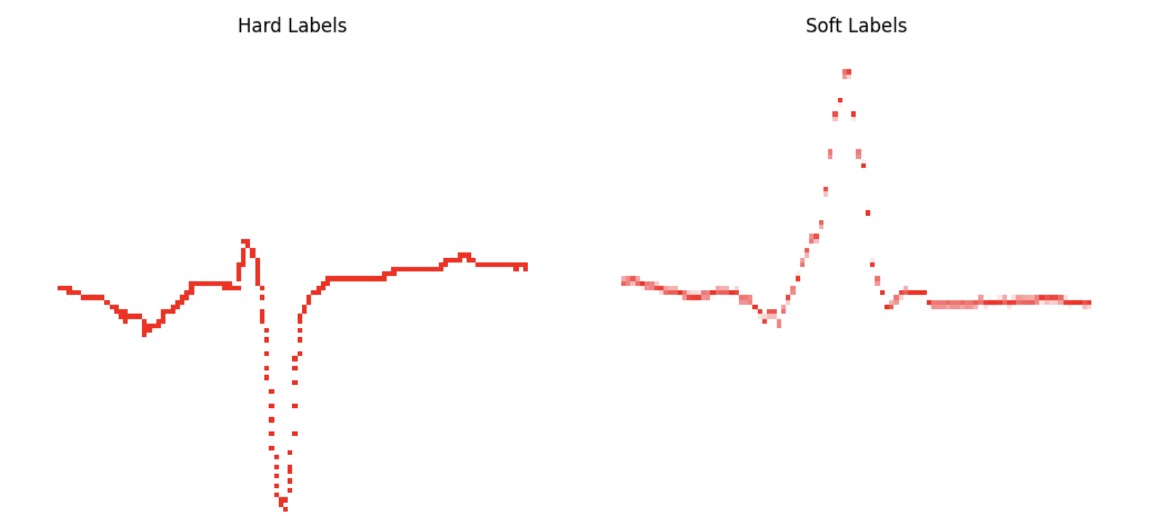\n\n**Dual Mode Training**\n\nFor Stage D, I used essentially the same model as the original stage2 model with the exception that whereas the original model adds the y coordinates of the image into the final layer of the network, I add both the x and y coordinates. This makes it a challenge to do spatial augmentations, such as rotations or perspective shifts as both make it difficult to set the x and y coordinates properly. To get around this, during training I trained the network both before and after the final layer with 0.5 probability. When training before the final layer, I would do the more problematic rotation and perspective shift augmentations. When training after the final layer, I would only do augmentations, such as horizontal translation and color shifts.",
"votes": null
},
{
"id": "3396110",
"postDate": "01/24/2026 10:52:27",
"content": "Thanks for sharing. We tried signal segmentation as well but it did not work well as we expected. How do you get hard label? Did you used rectified images of all types for training ?
", "rawMarkdown": "Thanks for sharing. We tried signal segmentation as well but it did not work well as we expected. How do you get hard label? Did you used rectified images of all types for training ?", "votes": null }, { "id": "3396152", "postDate": "01/24/2026 12:47:35", "content": "Hi @vandongtran, thanks for reading. I need to add a few more sections still to cover augmentations and training, but I trained using rectified images of all types with augmentations including grayscale, contrast adjustment, mold simulation, and blur. One thing I noticed was that I initially got better results using the rougher rectified images without gridpoint refinement (training only) suggesting maybe the jitter in the grid acted as its own augmentation. I added the \"dual mode training\" as a way to add mild spatial augmentations without messing up the xcoord and ycoord inputs which seemed to help with the refined images. I'm not sure I understand your question about the hard labels. I used soft labels to encode the sub-pixel location of the signal. I included the image of the hard labels just to show the difference.
", "rawMarkdown": "Hi @vandongtran, thanks for reading. I need to add a few more sections still to cover augmentations and training, but I trained using rectified images of all types with augmentations including grayscale, contrast adjustment, mold simulation, and blur. One thing I noticed was that I initially got better results using the rougher rectified images without gridpoint refinement (training only) suggesting maybe the jitter in the grid acted as its own augmentation. I added the \"dual mode training\" as a way to add mild spatial augmentations without messing up the xcoord and ycoord inputs which seemed to help with the refined images. I'm not sure I understand your question about the hard labels. I used soft labels to encode the sub-pixel location of the signal. I included the image of the hard labels just to show the difference.", "votes": null }, { "id": "3396156", "postDate": "01/24/2026 13:00:02", "content": "@davidlist Thanks for your answer. Regarding the hard labels, if I understand correctly, they are binary masks for signal segmentation. I was wondering how you obtained them (i.e., how they were generated? from the ground-truth signal?)
", "rawMarkdown": "davidlist Thanks for your answer. Regarding the hard labels, if I understand correctly, they are binary masks for signal segmentation. I was wondering how you obtained them (i.e., how they were generated? from the ground-truth signal?)", "votes": null }, { "id": "3396172", "postDate": "01/24/2026 13:28:06", "content": "Ahh… Sorry, I understand now. I hacked the ecg-image-kit code to plot the labels instead of the ecgs.
", "rawMarkdown": "Ahh... Sorry, I understand now. I hacked the ecg-image-kit code to plot the labels instead of the ecgs.", "votes": null }, { "id": "3396176", "postDate": "01/24/2026 13:37:26", "content": "We used them as well, but did you also apply the rectification stage to the masks so they align with the rectified images?
\nWhen I overlay the masks obtained from ECG-image-kit onto the rectified images, the mask and the actual signal are misaligned near the end of the image—the further to the right it goes, the more misaligned it becomes.
\nOr did you train the segmentation model using the original masks from ECG-image-kit together with the rectified images, and simply allow the misalignment?
", "rawMarkdown": "We used them as well, but did you also apply the rectification stage to the masks so they align with the rectified images?\n\nWhen I overlay the masks obtained from ECG-image-kit onto the rectified images, the mask and the actual signal are misaligned near the end of the image—the further to the right it goes, the more misaligned it becomes.\n\nOr did you train the segmentation model using the original masks from ECG-image-kit together with the rectified images, and simply allow the misalignment?", "votes": null }, { "id": "3396183", "postDate": "01/24/2026 13:47:51", "content": "No, you're right. I ran into the same problem. Took me awhile to realize the two grids were different, but I ended up regenerating the labels using the rectification grid. It actually gets even a little more complicated than that, because ecg-image-kit plots the signals continuously, but the grid discretely meaning sometimes the grid is actually off by a pixel, but I decided to ignore this second problem.
", "rawMarkdown": "No, you're right. I ran into the same problem. Took me awhile to realize the two grids were different, but I ended up regenerating the labels using the rectification grid. It actually gets even a little more complicated than that, because ecg-image-kit plots the signals continuously, but the grid discretely meaning sometimes the grid is actually off by a pixel, but I decided to ignore this second problem.", "votes": null }, { "id": "3396194", "postDate": "01/24/2026 14:01:54", "content": "Oh, I’d really like to learn more details about your work, since we use a very similar segmentation pipeline but our model did not achieve an SNR comparable to yours.
\nIf you’re able to share the code, that would be great for us to learn from. Also, do you know what SNR score your ground-truth masks achieve?
", "rawMarkdown": "Oh, I’d really like to learn more details about your work, since we use a very similar segmentation pipeline but our model did not achieve an SNR comparable to yours.\n\nIf you’re able to share the code, that would be great for us to learn from. Also, do you know what SNR score your ground-truth masks achieve?", "votes": null }, { "id": "3396581", "postDate": "01/25/2026 10:58:11", "content": "I never calculated the SNR score, but that's a great idea. I believe this is my notebook for hard labels at 2200x1700 resolution on the rectified grid. This isn't what I actually used for my final submission, of course: https://www.kaggle.com/code/davidlist/stage-d-rectified-labels. And then this second should be what I actually used: https://www.kaggle.com/code/davidlist/high-res-label-generator-2x1. These are the soft labels at 4400x1696 resolution.
", "rawMarkdown": "I never calculated the SNR score, but that's a great idea. I believe this is my notebook for hard labels at 2200x1700 resolution on the rectified grid. This isn't what I actually used for my final submission, of course: [https://www.kaggle.com/code/davidlist/stage-d-rectified-labels](https://www.kaggle.com/code/davidlist/stage-d-rectified-labels). And then this second should be what I actually used: [https://www.kaggle.com/code/davidlist/high-res-label-generator-2x1](https://www.kaggle.com/code/davidlist/high-res-label-generator-2x1). These are the soft labels at 4400x1696 resolution.", "votes": null } ], "comments": [ { "id": 3396110, "author_name": "vandongtran", "author_url": "", "post_date": "01/24/2026 10:52:27", "content": "Thanks for sharing. We tried signal segmentation as well but it did not work well as we expected. How do you get hard label? Did you used rectified images of all types for training ?
", "votes": null, "replies": [ { "id": 3396152, "author_name": "davidlist", "author_url": "", "post_date": "01/24/2026 12:47:35", "content": "Hi @vandongtran, thanks for reading. I need to add a few more sections still to cover augmentations and training, but I trained using rectified images of all types with augmentations including grayscale, contrast adjustment, mold simulation, and blur. One thing I noticed was that I initially got better results using the rougher rectified images without gridpoint refinement (training only) suggesting maybe the jitter in the grid acted as its own augmentation. I added the \"dual mode training\" as a way to add mild spatial augmentations without messing up the xcoord and ycoord inputs which seemed to help with the refined images. I'm not sure I understand your question about the hard labels. I used soft labels to encode the sub-pixel location of the signal. I included the image of the hard labels just to show the difference.
", "votes": null, "replies": [ { "id": 3396156, "author_name": "vandongtran", "author_url": "", "post_date": "01/24/2026 13:00:02", "content": "@davidlist Thanks for your answer. Regarding the hard labels, if I understand correctly, they are binary masks for signal segmentation. I was wondering how you obtained them (i.e., how they were generated? from the ground-truth signal?)
", "votes": null, "replies": [ { "id": 3396172, "author_name": "davidlist", "author_url": "", "post_date": "01/24/2026 13:28:06", "content": "Ahh… Sorry, I understand now. I hacked the ecg-image-kit code to plot the labels instead of the ecgs.
", "votes": null, "replies": [ { "id": 3396176, "author_name": "vandongtran", "author_url": "", "post_date": "01/24/2026 13:37:26", "content": "We used them as well, but did you also apply the rectification stage to the masks so they align with the rectified images?
\nWhen I overlay the masks obtained from ECG-image-kit onto the rectified images, the mask and the actual signal are misaligned near the end of the image—the further to the right it goes, the more misaligned it becomes.
\nOr did you train the segmentation model using the original masks from ECG-image-kit together with the rectified images, and simply allow the misalignment?
", "votes": null, "replies": [ { "id": 3396183, "author_name": "davidlist", "author_url": "", "post_date": "01/24/2026 13:47:51", "content": "No, you're right. I ran into the same problem. Took me awhile to realize the two grids were different, but I ended up regenerating the labels using the rectification grid. It actually gets even a little more complicated than that, because ecg-image-kit plots the signals continuously, but the grid discretely meaning sometimes the grid is actually off by a pixel, but I decided to ignore this second problem.
", "votes": null, "replies": [ { "id": 3396194, "author_name": "vandongtran", "author_url": "", "post_date": "01/24/2026 14:01:54", "content": "Oh, I’d really like to learn more details about your work, since we use a very similar segmentation pipeline but our model did not achieve an SNR comparable to yours.
\nIf you’re able to share the code, that would be great for us to learn from. Also, do you know what SNR score your ground-truth masks achieve?
", "votes": null, "replies": [ { "id": 3396581, "author_name": "davidlist", "author_url": "", "post_date": "01/25/2026 10:58:11", "content": "I never calculated the SNR score, but that's a great idea. I believe this is my notebook for hard labels at 2200x1700 resolution on the rectified grid. This isn't what I actually used for my final submission, of course: https://www.kaggle.com/code/davidlist/stage-d-rectified-labels. And then this second should be what I actually used: https://www.kaggle.com/code/davidlist/high-res-label-generator-2x1. These are the soft labels at 4400x1696 resolution.
", "votes": null, "replies": [] } ] } ] } ] } ] } ] } ] } ] } ], "raw_markdown_by_id": { "3395696": "Thank you to PhysioNet, the competition host, Kaggle, and everyone else involved for putting together such a challenging and interesting competition. Before entering this competition, I probably would have laughed off even the idea of doing this as magic so it is very gratifying to come away understanding a practical application of computer vision that I didn't realize was possible.\n\nSpecial thanks to @hengck23 and also @kami1976 whose notebooks provided the initial starting point of my solution. Also thank you to whoever came up with the algorithm for Einthoven error correction which I apply to my signals at the very end, @antonoof maybe?\n\nAs suggested by my subtitle, my solution is for the most part an extension of hengck23's original [demo submission](https://www.kaggle.com/code/hengck23/demo-submission) notebook, although I do provide some significant changes. The following sections describe the basic flow of my inference pipeline.\n\n\n\n**Stage A - Orientation**\n\nIn the first stage of my pipeline I call the first part of @hengck23's stage0's model to get a properly oriented image and the location of its key point markers.\n\n**Stage B - Homography**\n\n@hengck23's stage0 uses homography to warp and output a canonical image at 1440x1152 resolution which is significantly lower than the 2200x1700 ecg images generated by ecg-image-kit. In Stage B, I create both that lower resolution image as well as a high resolution 2400x1920 image designed to preserve as much information as possible from the original ECG.\n\n**Stage C - Rectification**\n\nStage C consists of the following main steps:\n- Pass the low resolution 1440x1152 image from Stage B through @hengck23's stage0 model to get the grid point locations.\n- Convert those low resolution grid points into the coordinate system of the high resolution 2400x1920 image.\n- Pass the high resolution grid points through a cascade of refinement neural networks to refine their positions to (hopefully) sub-pixel accuracy.\n- Perform rectification on the high resolution image with the refined grid points.\n\n**Stage D - Signal Extraction**\n\nI follow essentially the same process as in the [demo submission](https://www.kaggle.com/code/hengck23/demo-submission) notebook with the following exceptions:\n- Instead of performing it on the original image, I scale the image to twice it's length as recommended by @hengck23 in one of the [discussion posts.](https://www.kaggle.com/competitions/physionet-ecg-image-digitization/discussion/624054). Note, that I actually tried various resolutions, 2x2, 1x2, 1x4, and 1x8, but 1x2 pretty easily outperforms the others.\n- Because I use soft labels, I extract the signal using weighted averaging of a window around argmax. Surprisingly, a window of 100 pixels in each direction worked best with diminishing returns after that. Likely this does a better job of estimating the QRS spikes.\n- The image is processed in patches and passed through an ensemble of 10 models trained with different random seeds.\n\n**Stage E - Post Processing**\n\nFor post processing I do two things:\n- I ensemble the first 1/4 of the long II lead with the short II lead.\n- I use the Einthoven error correction algorithm found in several of the public notebooks.\n\n**Grid Point Refinement**\n\nThe grid point detection in the [demo submission notebook](https://www.kaggle.com/code/hengck23/demo-submission) is good, but not perfect. If you look closely at the image on the left you can see small deformations in the ECG grid where the grid point detection is off by a pixel or two. These deformations, of course, directly impact signal accuracy so getting them as accurate as possible helps SNR. As mentioned above, I used the @hengck23's stage1 network to initially predict the image gridpoints, then I passed each gridpoint through a cascade of two refinement networks to locate each as accurately as possible. The image on the right shows the resulting grid which is nearly perfect.\n\n| Before | \nAfter | \n
| \n | \n
\n\n**Soft Labels**\n\nInstead of using hard labels where a pixel is set to either 0 or 1, I used soft labels such that the intensity of the two adjacent pixels between which the signal passes is set related to how close the signal is to the center of each. For instance if the signal is 0.1 pixels distant from the first pixel's center, it gets a value of 0.9 whereas the adjacent pixel gets a value of 0.1. The value of soft labels over hard labels in this case is it allows the labels to be specified at sub-pixel resolution. The following image shows hard and soft labels.\n\n\n\n**Dual Mode Training**\n\nFor Stage D, I used essentially the same model as the original stage2 model with the exception that whereas the original model adds the y coordinates of the image into the final layer of the network, I add both the x and y coordinates. This makes it a challenge to do spatial augmentations, such as rotations or perspective shifts as both make it difficult to set the x and y coordinates properly. To get around this, during training I trained the network both before and after the final layer with 0.5 probability. When training before the final layer, I would do the more problematic rotation and perspective shift augmentations. When training after the final layer, I would only do augmentations, such as horizontal translation and color shifts.",
"3396110": "Thanks for sharing. We tried signal segmentation as well but it did not work well as we expected. How do you get hard label? Did you used rectified images of all types for training ?",
"3396152": "Hi @vandongtran, thanks for reading. I need to add a few more sections still to cover augmentations and training, but I trained using rectified images of all types with augmentations including grayscale, contrast adjustment, mold simulation, and blur. One thing I noticed was that I initially got better results using the rougher rectified images without gridpoint refinement (training only) suggesting maybe the jitter in the grid acted as its own augmentation. I added the \"dual mode training\" as a way to add mild spatial augmentations without messing up the xcoord and ycoord inputs which seemed to help with the refined images. I'm not sure I understand your question about the hard labels. I used soft labels to encode the sub-pixel location of the signal. I included the image of the hard labels just to show the difference.",
"3396156": "davidlist Thanks for your answer. Regarding the hard labels, if I understand correctly, they are binary masks for signal segmentation. I was wondering how you obtained them (i.e., how they were generated? from the ground-truth signal?)",
"3396172": "Ahh... Sorry, I understand now. I hacked the ecg-image-kit code to plot the labels instead of the ecgs.",
"3396176": "We used them as well, but did you also apply the rectification stage to the masks so they align with the rectified images?\n\nWhen I overlay the masks obtained from ECG-image-kit onto the rectified images, the mask and the actual signal are misaligned near the end of the image—the further to the right it goes, the more misaligned it becomes.\n\nOr did you train the segmentation model using the original masks from ECG-image-kit together with the rectified images, and simply allow the misalignment?",
"3396183": "No, you're right. I ran into the same problem. Took me awhile to realize the two grids were different, but I ended up regenerating the labels using the rectification grid. It actually gets even a little more complicated than that, because ecg-image-kit plots the signals continuously, but the grid discretely meaning sometimes the grid is actually off by a pixel, but I decided to ignore this second problem.",
"3396194": "Oh, I’d really like to learn more details about your work, since we use a very similar segmentation pipeline but our model did not achieve an SNR comparable to yours.\n\nIf you’re able to share the code, that would be great for us to learn from. Also, do you know what SNR score your ground-truth masks achieve?",
"3396581": "I never calculated the SNR score, but that's a great idea. I believe this is my notebook for hard labels at 2200x1700 resolution on the rectified grid. This isn't what I actually used for my final submission, of course: [https://www.kaggle.com/code/davidlist/stage-d-rectified-labels](https://www.kaggle.com/code/davidlist/stage-d-rectified-labels). And then this second should be what I actually used: [https://www.kaggle.com/code/davidlist/high-res-label-generator-2x1](https://www.kaggle.com/code/davidlist/high-res-label-generator-2x1). These are the soft labels at 4400x1696 resolution."
},
"source": "meta"
}