{
  "id": 669594,
  "title": "12th place solution",
  "url": "/competitions/physionet-ecg-image-digitization/writeups/12th-place-solution",
  "author_name": "",
  "post_date": "2026-01-23T09:07:20.773Z",
  "votes": 16,
  "comment_count": 2,
  "views": 0,
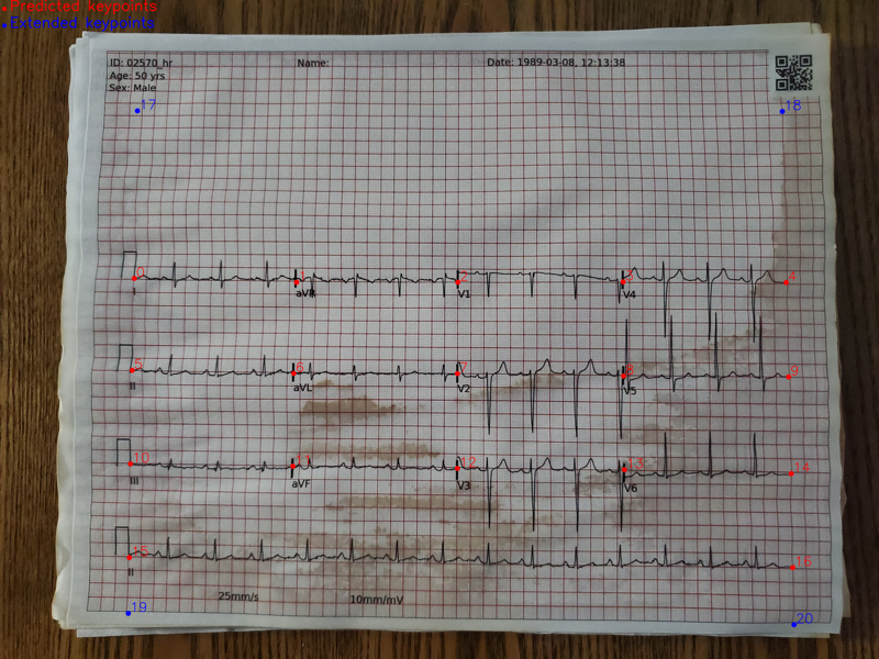
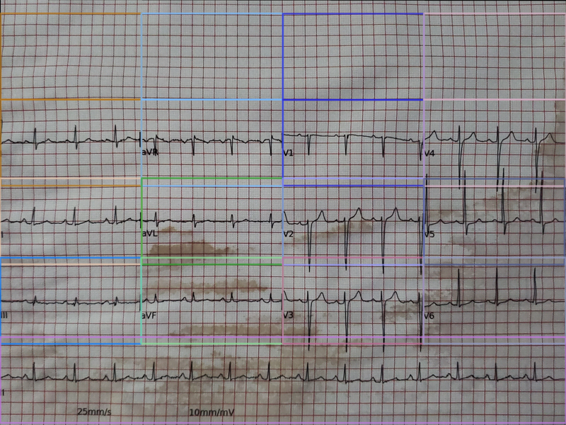
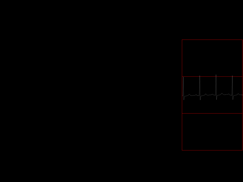
  "content": "<h2>Acknowledgements</h2>\n<p>We would like to thank Kaggle and the competition organizers for providing the dataset and the opportunity to participate. We also appreciate the community for discussions and sharing ideas that helped improve our approach.</p>\n<hr>\n<h2>1. Overall Pipeline</h2>\n<ol>\n<li>Orientation detection and correction using OCR</li>\n<li>Detect the paper region using OpenCV and crop it</li>\n<li>Detect 17 grid points using a keypoint detection model</li>\n<li>For the 17 detected keypoints, extend the four corner keypoints and add four additional points. Then, Delaunay triangulation is applied to a predefined Type1 keypoint layout, and each triangular region from the target image, defined by the corresponding detected keypoints, is warped onto this layout. To reduce information loss for high-resolution images, the reference keypoints are upscaled by ×2 during warping (as shown in the figures below).</li>\n<li>Crop each lead region from the result of step 4, and predict the signal for each lead using a signal extraction model.</li>\n</ol>\n<ul>\n<li><p>Visualization of predicted and extended keypoints.<br>\n<img src=\"https://www.googleapis.com/download/storage/v1/b/kaggle-user-content/o/inbox%2F1864394%2F286718b8b4497c3bcedad6e29c9389c8%2Fphysionet_writeup_kpt_det.png?generation=1769157091129433&amp;alt=media\" alt=\"\"></p></li>\n<li><p>Visualization showing the image after Delaunay triangulation and warping. The bounding boxes indicate each lead's ROI used as model input.<br>\n<img src=\"https://www.googleapis.com/download/storage/v1/b/kaggle-user-content/o/inbox%2F1864394%2F8c3fd7d870326ea6e1b6eb453663c443%2Fphysionet_writeup_warped.png?generation=1769157242443396&amp;alt=media\" alt=\"\"></p></li>\n</ul>\n<hr>\n<h2>2. Data</h2>\n<p>Only competition data was used (no external or synthetic data).</p>\n<hr>\n<h2>3. Grid Keypoint Detection</h2>\n<ol>\n<li>Predict 17 individual keypoint masks (17 output channels) using a segmentation model.</li>\n<li>Extract keypoint coordinates using connected components (<code>scipy.ndimage.label</code>) with weighted average.</li>\n</ol>\n<h3>Model Architecture</h3>\n<p>A simple U-Net segmentation model with a <code>convnext_small.dinov3_lvd1689m</code> backbone, an additional decoder-head for PAF auxiliary loss, and an orientation detection head.  </p>\n<h3>Loss</h3>\n<p>Hybrid loss consisting of:</p>\n<ul>\n<li>Dice Loss  </li>\n<li>BCE Loss  </li>\n<li>PAF Loss  </li>\n<li>Cross-Entropy Loss for orientation classification  </li>\n</ul>\n<h3>Training Process</h3>\n<ol>\n<li>Repeat the following process for N = 350, 450, …, 700:<ul>\n<li>Manually annotate 17 grid keypoints for N images</li>\n<li>Train the model using images with manually annotated ground truth labels (initialize weights from previous checkpoint if available)</li>\n<li>Predict keypoints for all images and fine-tune the model using both ground truth and predicted pseudo keypoints</li></ul></li>\n<li>At this stage, accuracy was generally good except for the right edge points. Therefore, pseudo keypoints were imported back into the annotation tool, and only the wrongly predicted right-edge keypoints were manually corrected. The model was then fine-tuned using the complete annotation to obtain the final model.</li>\n</ol>\n<h3>Augmentation</h3>\n<ul>\n<li>OneOf:<ul>\n<li>ElasticTransform</li>\n<li>GridDistortion</li>\n<li>OpticalDistortion</li></ul></li>\n<li>OneOf:<ul>\n<li>ShiftScaleRotate</li>\n<li>Perspective</li></ul></li>\n<li>RandomBrightnessContrast</li>\n<li>GaussianNoise</li>\n<li>ImageCompression</li>\n<li>CoarseDropout</li>\n<li>Rotation 90/180/270 degrees</li>\n</ul>\n<hr>\n<h2>4. Signal Extraction</h2>\n<ol>\n<li>Signal segmentation using a U-Net segmentation module</li>\n<li>Apply warping to the mask using a learnable warp field (output of another U-Net decoder branch) via 2D grid sampling</li>\n<li>Predict signal time series from the warped segmentation mask using a 1D CNN-based regression head</li>\n<li>Resample to 2.5× sampling frequency using a learnable optimized resampler with 1D grid sampling</li>\n</ol>\n<p>All modules above were trained jointly.<br>\nSince phase shifts caused by resampling were significant, I introduced a learnable resampler to optimize resampling.<br>\n(For example, in experiments where only the last point of the final predicted <code>number_of_rows</code> was trimmed or padded and then interpolated back to <code>number_of_rows</code>, the public LB degraded from 21.49 → 20.12/20.00.)</p>\n<h3>Model Architecture</h3>\n<p><img src=\"https://www.googleapis.com/download/storage/v1/b/kaggle-user-content/o/inbox%2F1864394%2F9b2e772b4c73e0bc1a2581e2f51b99f0%2Fdiagram.svg?generation=1769156635651095&amp;alt=media\"></p>\n<ul>\n<li>Backbone: <code>convnext_tiny.dinov3_lvd1689m</code> / <code>convnext_small.dinov3_lvd1689m</code></li>\n</ul>\n<h3>Loss</h3>\n<p>Hybrid loss consisting of:</p>\n<ul>\n<li>Dice Loss for signal segmentation</li>\n<li>BCE Loss for signal segmentation</li>\n<li>SNR Loss for signal regression</li>\n<li>Warp smoothness loss for grid warping regularization</li>\n</ul>\n<h3>Augmentation</h3>\n<ul>\n<li>OneOf:<ul>\n<li>ElasticTransform</li>\n<li>GridDistortion</li>\n<li>OpticalDistortion</li></ul></li>\n<li>RandomBrightnessContrast</li>\n<li>GaussianNoise</li>\n<li>ImageCompression</li>\n<li>CoarseDropout</li>\n<li>Use pseudo (predicted) keypoints instead of ground truth (manual) keypoints for region cropping</li>\n<li>Add Gaussian noise to keypoint coordinates</li>\n<li>Additional right edge keypoint noise</li>\n<li>Randomly select sampling frequency and resample GT signal</li>\n</ul>\n<p><strong>Note:</strong> The above augmentations are not applied to signal segmentation ground truth masks. The goal is to make the model learn distortion correction via the warping module.</p>\n<h3>Preprocessing / Training</h3>\n<ul>\n<li>For model input images, crop each lead's ROI using GT/predicted keypoints with constant height. Resize each to <code>(3, H_lead=384, W_LEAD=1536)</code> and stack to <code>(n_leads=16, 3, H_lead, W_LEAD)</code>. Additionally, top region images <code>(n_leads_top=4, 3, H_lead, W_LEAD)</code> are prepared similarly.</li>\n<li>For signal segmentation GT masks, after drawing the mask of the target lead, the target region including <code>y=0</code> and ±1 regions (as shown in the figure below) is cropped and resized to <code>(3, 3 × H_lead=1152, W_LEAD=1536)</code>, then stacked for all leads to <code>(n_leads=16, 3, 3×H_lead, W_LEAD)</code>.</li>\n<li>To handle cases where the signal extends beyond the target lead region, the model concatenates features from adjacent y ±1 regions in the encoder feature space, so the final single-lead predicted segmentation height is <code>3×H_lead</code>, matching the GT mask.</li>\n</ul>\n<p>GT mask example for the V5 lead. The red bounding box indicates the cropped region used for training.\n<img src=\"https://www.googleapis.com/download/storage/v1/b/kaggle-user-content/o/inbox%2F1864394%2F168c94a45eb791b15a8c4edbf1e3550a%2Fphysionet_writeup_gt_mask.png?generation=1769156856812096&amp;alt=media\" alt=\"\"></p>\n<hr>\n<h2>5. Ensemble</h2>\n<p>A simple weighted average ensemble worked best.<br>\nUltimately, three models (grid keypoint detection model was a single model) were used. With 90-degree rotation TTA, a total of 3 × 2 = 6 predictions were combined via weighted average for the best result.</p>\n<ul>\n<li>Single models</li>\n</ul>\n<table>\n<thead>\n<tr>\n<th>Model Name</th>\n<th>Backbone</th>\n<th>Use FS PE</th>\n<th>Public LB</th>\n<th>Private LB</th>\n</tr>\n</thead>\n<tbody>\n<tr>\n<td>A</td>\n<td>convnext_tiny.dinov3_lvd1689m</td>\n<td>No</td>\n<td>21.49</td>\n<td>21.18</td>\n</tr>\n<tr>\n<td>B</td>\n<td>convnext_small.dinov3_lvd1689m</td>\n<td>Yes</td>\n<td>21.12</td>\n<td>20.84</td>\n</tr>\n<tr>\n<td>C (derived from A)</td>\n<td>convnext_tiny.dinov3_lvd1689m</td>\n<td>No</td>\n<td>21.36</td>\n<td>21.03</td>\n</tr>\n</tbody>\n</table>\n<ul>\n<li>Ensemble</li>\n</ul>\n<table>\n<thead>\n<tr>\n<th>No</th>\n<th>A weight</th>\n<th>B weight</th>\n<th>C weight</th>\n<th>(Keypoint Detection) Rot90 TTA</th>\n<th>Public LB</th>\n<th>Private LB</th>\n</tr>\n</thead>\n<tbody>\n<tr>\n<td>1</td>\n<td>0.45</td>\n<td>0.4</td>\n<td>0.15</td>\n<td>Yes</td>\n<td>21.86</td>\n<td>21.57</td>\n</tr>\n<tr>\n<td>2</td>\n<td>0.4</td>\n<td>0.4</td>\n<td>0.2</td>\n<td>No</td>\n<td>21.81</td>\n<td>21.50</td>\n</tr>\n<tr>\n<td>3</td>\n<td>0.5</td>\n<td>0.2</td>\n<td>0.3</td>\n<td>No</td>\n<td>21.76</td>\n<td>21.45</td>\n</tr>\n</tbody>\n</table>",
  "messages": [
    {
      "id": "3395577",
      "postDate": "01/23/2026 08:56:26",
      "content": "<h2>Acknowledgements</h2>\n<p>We would like to thank Kaggle and the competition organizers for providing the dataset and the opportunity to participate. We also appreciate the community for discussions and sharing ideas that helped improve our approach.</p>\n<hr>\n<h2>1. Overall Pipeline</h2>\n<ol>\n<li>Orientation detection and correction using OCR</li>\n<li>Detect the paper region using OpenCV and crop it</li>\n<li>Detect 17 grid points using a keypoint detection model</li>\n<li>For the 17 detected keypoints, extend the four corner keypoints and add four additional points. Then, Delaunay triangulation is applied to a predefined Type1 keypoint layout, and each triangular region from the target image, defined by the corresponding detected keypoints, is warped onto this layout. To reduce information loss for high-resolution images, the reference keypoints are upscaled by ×2 during warping (as shown in the figures below).</li>\n<li>Crop each lead region from the result of step 4, and predict the signal for each lead using a signal extraction model.</li>\n</ol>\n<ul>\n<li><p>Visualization of predicted and extended keypoints.<br>\n<img src=\"https://www.googleapis.com/download/storage/v1/b/kaggle-user-content/o/inbox%2F1864394%2F286718b8b4497c3bcedad6e29c9389c8%2Fphysionet_writeup_kpt_det.png?generation=1769157091129433&amp;alt=media\" alt=\"\"></p></li>\n<li><p>Visualization showing the image after Delaunay triangulation and warping. The bounding boxes indicate each lead's ROI used as model input.<br>\n<img src=\"https://www.googleapis.com/download/storage/v1/b/kaggle-user-content/o/inbox%2F1864394%2F8c3fd7d870326ea6e1b6eb453663c443%2Fphysionet_writeup_warped.png?generation=1769157242443396&amp;alt=media\" alt=\"\"></p></li>\n</ul>\n<hr>\n<h2>2. Data</h2>\n<p>Only competition data was used (no external or synthetic data).</p>\n<hr>\n<h2>3. Grid Keypoint Detection</h2>\n<ol>\n<li>Predict 17 individual keypoint masks (17 output channels) using a segmentation model.</li>\n<li>Extract keypoint coordinates using connected components (<code>scipy.ndimage.label</code>) with weighted average.</li>\n</ol>\n<h3>Model Architecture</h3>\n<p>A simple U-Net segmentation model with a <code>convnext_small.dinov3_lvd1689m</code> backbone, an additional decoder-head for PAF auxiliary loss, and an orientation detection head.  </p>\n<h3>Loss</h3>\n<p>Hybrid loss consisting of:</p>\n<ul>\n<li>Dice Loss  </li>\n<li>BCE Loss  </li>\n<li>PAF Loss  </li>\n<li>Cross-Entropy Loss for orientation classification  </li>\n</ul>\n<h3>Training Process</h3>\n<ol>\n<li>Repeat the following process for N = 350, 450, …, 700:<ul>\n<li>Manually annotate 17 grid keypoints for N images</li>\n<li>Train the model using images with manually annotated ground truth labels (initialize weights from previous checkpoint if available)</li>\n<li>Predict keypoints for all images and fine-tune the model using both ground truth and predicted pseudo keypoints</li></ul></li>\n<li>At this stage, accuracy was generally good except for the right edge points. Therefore, pseudo keypoints were imported back into the annotation tool, and only the wrongly predicted right-edge keypoints were manually corrected. The model was then fine-tuned using the complete annotation to obtain the final model.</li>\n</ol>\n<h3>Augmentation</h3>\n<ul>\n<li>OneOf:<ul>\n<li>ElasticTransform</li>\n<li>GridDistortion</li>\n<li>OpticalDistortion</li></ul></li>\n<li>OneOf:<ul>\n<li>ShiftScaleRotate</li>\n<li>Perspective</li></ul></li>\n<li>RandomBrightnessContrast</li>\n<li>GaussianNoise</li>\n<li>ImageCompression</li>\n<li>CoarseDropout</li>\n<li>Rotation 90/180/270 degrees</li>\n</ul>\n<hr>\n<h2>4. Signal Extraction</h2>\n<ol>\n<li>Signal segmentation using a U-Net segmentation module</li>\n<li>Apply warping to the mask using a learnable warp field (output of another U-Net decoder branch) via 2D grid sampling</li>\n<li>Predict signal time series from the warped segmentation mask using a 1D CNN-based regression head</li>\n<li>Resample to 2.5× sampling frequency using a learnable optimized resampler with 1D grid sampling</li>\n</ol>\n<p>All modules above were trained jointly.<br>\nSince phase shifts caused by resampling were significant, I introduced a learnable resampler to optimize resampling.<br>\n(For example, in experiments where only the last point of the final predicted <code>number_of_rows</code> was trimmed or padded and then interpolated back to <code>number_of_rows</code>, the public LB degraded from 21.49 → 20.12/20.00.)</p>\n<h3>Model Architecture</h3>\n<p><img src=\"https://www.googleapis.com/download/storage/v1/b/kaggle-user-content/o/inbox%2F1864394%2F9b2e772b4c73e0bc1a2581e2f51b99f0%2Fdiagram.svg?generation=1769156635651095&amp;alt=media\"></p>\n<ul>\n<li>Backbone: <code>convnext_tiny.dinov3_lvd1689m</code> / <code>convnext_small.dinov3_lvd1689m</code></li>\n</ul>\n<h3>Loss</h3>\n<p>Hybrid loss consisting of:</p>\n<ul>\n<li>Dice Loss for signal segmentation</li>\n<li>BCE Loss for signal segmentation</li>\n<li>SNR Loss for signal regression</li>\n<li>Warp smoothness loss for grid warping regularization</li>\n</ul>\n<h3>Augmentation</h3>\n<ul>\n<li>OneOf:<ul>\n<li>ElasticTransform</li>\n<li>GridDistortion</li>\n<li>OpticalDistortion</li></ul></li>\n<li>RandomBrightnessContrast</li>\n<li>GaussianNoise</li>\n<li>ImageCompression</li>\n<li>CoarseDropout</li>\n<li>Use pseudo (predicted) keypoints instead of ground truth (manual) keypoints for region cropping</li>\n<li>Add Gaussian noise to keypoint coordinates</li>\n<li>Additional right edge keypoint noise</li>\n<li>Randomly select sampling frequency and resample GT signal</li>\n</ul>\n<p><strong>Note:</strong> The above augmentations are not applied to signal segmentation ground truth masks. The goal is to make the model learn distortion correction via the warping module.</p>\n<h3>Preprocessing / Training</h3>\n<ul>\n<li>For model input images, crop each lead's ROI using GT/predicted keypoints with constant height. Resize each to <code>(3, H_lead=384, W_LEAD=1536)</code> and stack to <code>(n_leads=16, 3, H_lead, W_LEAD)</code>. Additionally, top region images <code>(n_leads_top=4, 3, H_lead, W_LEAD)</code> are prepared similarly.</li>\n<li>For signal segmentation GT masks, after drawing the mask of the target lead, the target region including <code>y=0</code> and ±1 regions (as shown in the figure below) is cropped and resized to <code>(3, 3 × H_lead=1152, W_LEAD=1536)</code>, then stacked for all leads to <code>(n_leads=16, 3, 3×H_lead, W_LEAD)</code>.</li>\n<li>To handle cases where the signal extends beyond the target lead region, the model concatenates features from adjacent y ±1 regions in the encoder feature space, so the final single-lead predicted segmentation height is <code>3×H_lead</code>, matching the GT mask.</li>\n</ul>\n<p>GT mask example for the V5 lead. The red bounding box indicates the cropped region used for training.\n<img src=\"https://www.googleapis.com/download/storage/v1/b/kaggle-user-content/o/inbox%2F1864394%2F168c94a45eb791b15a8c4edbf1e3550a%2Fphysionet_writeup_gt_mask.png?generation=1769156856812096&amp;alt=media\" alt=\"\"></p>\n<hr>\n<h2>5. Ensemble</h2>\n<p>A simple weighted average ensemble worked best.<br>\nUltimately, three models (grid keypoint detection model was a single model) were used. With 90-degree rotation TTA, a total of 3 × 2 = 6 predictions were combined via weighted average for the best result.</p>\n<ul>\n<li>Single models</li>\n</ul>\n<table>\n<thead>\n<tr>\n<th>Model Name</th>\n<th>Backbone</th>\n<th>Use FS PE</th>\n<th>Public LB</th>\n<th>Private LB</th>\n</tr>\n</thead>\n<tbody>\n<tr>\n<td>A</td>\n<td>convnext_tiny.dinov3_lvd1689m</td>\n<td>No</td>\n<td>21.49</td>\n<td>21.18</td>\n</tr>\n<tr>\n<td>B</td>\n<td>convnext_small.dinov3_lvd1689m</td>\n<td>Yes</td>\n<td>21.12</td>\n<td>20.84</td>\n</tr>\n<tr>\n<td>C (derived from A)</td>\n<td>convnext_tiny.dinov3_lvd1689m</td>\n<td>No</td>\n<td>21.36</td>\n<td>21.03</td>\n</tr>\n</tbody>\n</table>\n<ul>\n<li>Ensemble</li>\n</ul>\n<table>\n<thead>\n<tr>\n<th>No</th>\n<th>A weight</th>\n<th>B weight</th>\n<th>C weight</th>\n<th>(Keypoint Detection) Rot90 TTA</th>\n<th>Public LB</th>\n<th>Private LB</th>\n</tr>\n</thead>\n<tbody>\n<tr>\n<td>1</td>\n<td>0.45</td>\n<td>0.4</td>\n<td>0.15</td>\n<td>Yes</td>\n<td>21.86</td>\n<td>21.57</td>\n</tr>\n<tr>\n<td>2</td>\n<td>0.4</td>\n<td>0.4</td>\n<td>0.2</td>\n<td>No</td>\n<td>21.81</td>\n<td>21.50</td>\n</tr>\n<tr>\n<td>3</td>\n<td>0.5</td>\n<td>0.2</td>\n<td>0.3</td>\n<td>No</td>\n<td>21.76</td>\n<td>21.45</td>\n</tr>\n</tbody>\n</table>",
      "rawMarkdown": "## Acknowledgements\n\nWe would like to thank Kaggle and the competition organizers for providing the dataset and the opportunity to participate. We also appreciate the community for discussions and sharing ideas that helped improve our approach.\n\n---\n\n## 1. Overall Pipeline\n\n1. Orientation detection and correction using OCR\n2. Detect the paper region using OpenCV and crop it\n3. Detect 17 grid points using a keypoint detection model\n4. For the 17 detected keypoints, extend the four corner keypoints and add four additional points. Then, Delaunay triangulation is applied to a predefined Type1 keypoint layout, and each triangular region from the target image, defined by the corresponding detected keypoints, is warped onto this layout. To reduce information loss for high-resolution images, the reference keypoints are upscaled by ×2 during warping (as shown in the figures below).\n5. Crop each lead region from the result of step 4, and predict the signal for each lead using a signal extraction model.\n\n- Visualization of predicted and extended keypoints.  \n![](https://www.googleapis.com/download/storage/v1/b/kaggle-user-content/o/inbox%2F1864394%2F286718b8b4497c3bcedad6e29c9389c8%2Fphysionet_writeup_kpt_det.png?generation=1769157091129433&alt=media)\n\n- Visualization showing the image after Delaunay triangulation and warping. The bounding boxes indicate each lead's ROI used as model input.  \n![](https://www.googleapis.com/download/storage/v1/b/kaggle-user-content/o/inbox%2F1864394%2F8c3fd7d870326ea6e1b6eb453663c443%2Fphysionet_writeup_warped.png?generation=1769157242443396&alt=media)\n\n---\n\n## 2. Data\n\nOnly competition data was used (no external or synthetic data).\n\n---\n\n## 3. Grid Keypoint Detection\n\n1. Predict 17 individual keypoint masks (17 output channels) using a segmentation model.\n2. Extract keypoint coordinates using connected components (`scipy.ndimage.label`) with weighted average.\n\n### Model Architecture\n\nA simple U-Net segmentation model with a `convnext_small.dinov3_lvd1689m` backbone, an additional decoder-head for PAF auxiliary loss, and an orientation detection head.  \n\n### Loss  \n\nHybrid loss consisting of:\n- Dice Loss  \n- BCE Loss  \n- PAF Loss  \n- Cross-Entropy Loss for orientation classification  \n\n### Training Process\n\n1. Repeat the following process for N = 350, 450, ..., 700:\n    - Manually annotate 17 grid keypoints for N images\n    - Train the model using images with manually annotated ground truth labels (initialize weights from previous checkpoint if available)\n    - Predict keypoints for all images and fine-tune the model using both ground truth and predicted pseudo keypoints\n2. At this stage, accuracy was generally good except for the right edge points. Therefore, pseudo keypoints were imported back into the annotation tool, and only the wrongly predicted right-edge keypoints were manually corrected. The model was then fine-tuned using the complete annotation to obtain the final model.\n\n### Augmentation\n\n- OneOf:\n    - ElasticTransform\n    - GridDistortion\n    - OpticalDistortion\n- OneOf:\n    - ShiftScaleRotate\n    - Perspective\n- RandomBrightnessContrast\n- GaussianNoise\n- ImageCompression\n- CoarseDropout\n- Rotation 90/180/270 degrees\n\n---\n\n## 4. Signal Extraction\n\n1. Signal segmentation using a U-Net segmentation module\n2. Apply warping to the mask using a learnable warp field (output of another U-Net decoder branch) via 2D grid sampling\n3. Predict signal time series from the warped segmentation mask using a 1D CNN-based regression head\n4. Resample to 2.5× sampling frequency using a learnable optimized resampler with 1D grid sampling\n\nAll modules above were trained jointly.  \nSince phase shifts caused by resampling were significant, I introduced a learnable resampler to optimize resampling.  \n(For example, in experiments where only the last point of the final predicted `number_of_rows` was trimmed or padded and then interpolated back to `number_of_rows`, the public LB degraded from 21.49 → 20.12/20.00.)\n\n### Model Architecture\n\n<img src=\"https://www.googleapis.com/download/storage/v1/b/kaggle-user-content/o/inbox%2F1864394%2F9b2e772b4c73e0bc1a2581e2f51b99f0%2Fdiagram.svg?generation=1769156635651095&alt=media\" width=\"600\">\n\n- Backbone: `convnext_tiny.dinov3_lvd1689m` / `convnext_small.dinov3_lvd1689m`\n\n### Loss  \n\nHybrid loss consisting of:\n- Dice Loss for signal segmentation\n- BCE Loss for signal segmentation\n- SNR Loss for signal regression\n- Warp smoothness loss for grid warping regularization\n\n### Augmentation\n\n- OneOf:\n    - ElasticTransform\n    - GridDistortion\n    - OpticalDistortion\n- RandomBrightnessContrast\n- GaussianNoise\n- ImageCompression\n- CoarseDropout\n- Use pseudo (predicted) keypoints instead of ground truth (manual) keypoints for region cropping\n- Add Gaussian noise to keypoint coordinates\n- Additional right edge keypoint noise\n- Randomly select sampling frequency and resample GT signal\n\n**Note:** The above augmentations are not applied to signal segmentation ground truth masks. The goal is to make the model learn distortion correction via the warping module.\n\n### Preprocessing / Training\n\n- For model input images, crop each lead's ROI using GT/predicted keypoints with constant height. Resize each to `(3, H_lead=384, W_LEAD=1536)` and stack to `(n_leads=16, 3, H_lead, W_LEAD)`. Additionally, top region images `(n_leads_top=4, 3, H_lead, W_LEAD)` are prepared similarly.\n- For signal segmentation GT masks, after drawing the mask of the target lead, the target region including `y=0` and ±1 regions (as shown in the figure below) is cropped and resized to `(3, 3 × H_lead=1152, W_LEAD=1536)`, then stacked for all leads to `(n_leads=16, 3, 3×H_lead, W_LEAD)`.\n- To handle cases where the signal extends beyond the target lead region, the model concatenates features from adjacent y ±1 regions in the encoder feature space, so the final single-lead predicted segmentation height is `3×H_lead`, matching the GT mask.\n\nGT mask example for the V5 lead. The red bounding box indicates the cropped region used for training.\n![](https://www.googleapis.com/download/storage/v1/b/kaggle-user-content/o/inbox%2F1864394%2F168c94a45eb791b15a8c4edbf1e3550a%2Fphysionet_writeup_gt_mask.png?generation=1769156856812096&alt=media)\n\n---\n\n## 5. Ensemble\n\nA simple weighted average ensemble worked best.  \nUltimately, three models (grid keypoint detection model was a single model) were used. With 90-degree rotation TTA, a total of 3 × 2 = 6 predictions were combined via weighted average for the best result.\n\n- Single models\n\n| Model Name | Backbone | Use FS PE | Public LB | Private LB |\n| ---- | ---- | ---- | ---- | ---- |\n| A | convnext_tiny.dinov3_lvd1689m | No | 21.49 | 21.18 |\n| B | convnext_small.dinov3_lvd1689m | Yes | 21.12 | 20.84 |\n| C (derived from A) | convnext_tiny.dinov3_lvd1689m | No | 21.36 | 21.03 |\n\n- Ensemble\n\n| No | A weight | B weight | C weight | (Keypoint Detection) Rot90 TTA | Public LB | Private LB |\n| ---- | ---- | ---- | ---- | ---- | ---- | ---- |\n| 1 | 0.45 | 0.4 | 0.15 | Yes | 21.86 | 21.57 |\n| 2 | 0.4 | 0.4 | 0.2 | No | 21.81 | 21.50 |\n| 3 | 0.5 | 0.2 | 0.3 | No | 21.76 | 21.45 |",
      "votes": null
    },
    {
      "id": "3395669",
      "postDate": "01/23/2026 12:35:06",
      "content": "<p>Finally, 😃.. somebody used OCR…I was thinking about using it…but couldn't do.. Congratulations 🎉</p>",
      "rawMarkdown": "Finally, 😃.. somebody used OCR...I was thinking about using it...but couldn't do.. Congratulations 🎉",
      "votes": null
    },
    {
      "id": "3494023",
      "postDate": "07/09/2026 01:09:20",
      "content": "<p><a href=\"https://www.kaggle.com/pondelion\" target=\"_blank\">@pondelion</a> can u please share any training or inferece code for this amazing top solution? i really want to appreciate how concise it is.</p>",
      "rawMarkdown": "pondelion can u please share any training or inferece code for this amazing top solution? i really want to appreciate how concise it is.",
      "votes": null
    }
  ],
  "comments": [
    {
      "id": 3395669,
      "author_name": "sanjidh090",
      "author_url": "",
      "post_date": "01/23/2026 12:35:06",
      "content": "<p>Finally, 😃.. somebody used OCR…I was thinking about using it…but couldn't do.. Congratulations 🎉</p>",
      "votes": null,
      "replies": []
    },
    {
      "id": 3494023,
      "author_name": "beckpro",
      "author_url": "",
      "post_date": "07/09/2026 01:09:20",
      "content": "<p><a href=\"https://www.kaggle.com/pondelion\" target=\"_blank\">@pondelion</a> can u please share any training or inferece code for this amazing top solution? i really want to appreciate how concise it is.</p>",
      "votes": null,
      "replies": []
    }
  ],
  "raw_markdown_by_id": {
    "3395577": "## Acknowledgements\n\nWe would like to thank Kaggle and the competition organizers for providing the dataset and the opportunity to participate. We also appreciate the community for discussions and sharing ideas that helped improve our approach.\n\n---\n\n## 1. Overall Pipeline\n\n1. Orientation detection and correction using OCR\n2. Detect the paper region using OpenCV and crop it\n3. Detect 17 grid points using a keypoint detection model\n4. For the 17 detected keypoints, extend the four corner keypoints and add four additional points. Then, Delaunay triangulation is applied to a predefined Type1 keypoint layout, and each triangular region from the target image, defined by the corresponding detected keypoints, is warped onto this layout. To reduce information loss for high-resolution images, the reference keypoints are upscaled by ×2 during warping (as shown in the figures below).\n5. Crop each lead region from the result of step 4, and predict the signal for each lead using a signal extraction model.\n\n- Visualization of predicted and extended keypoints.  \n![](https://www.googleapis.com/download/storage/v1/b/kaggle-user-content/o/inbox%2F1864394%2F286718b8b4497c3bcedad6e29c9389c8%2Fphysionet_writeup_kpt_det.png?generation=1769157091129433&alt=media)\n\n- Visualization showing the image after Delaunay triangulation and warping. The bounding boxes indicate each lead's ROI used as model input.  \n![](https://www.googleapis.com/download/storage/v1/b/kaggle-user-content/o/inbox%2F1864394%2F8c3fd7d870326ea6e1b6eb453663c443%2Fphysionet_writeup_warped.png?generation=1769157242443396&alt=media)\n\n---\n\n## 2. Data\n\nOnly competition data was used (no external or synthetic data).\n\n---\n\n## 3. Grid Keypoint Detection\n\n1. Predict 17 individual keypoint masks (17 output channels) using a segmentation model.\n2. Extract keypoint coordinates using connected components (`scipy.ndimage.label`) with weighted average.\n\n### Model Architecture\n\nA simple U-Net segmentation model with a `convnext_small.dinov3_lvd1689m` backbone, an additional decoder-head for PAF auxiliary loss, and an orientation detection head.  \n\n### Loss  \n\nHybrid loss consisting of:\n- Dice Loss  \n- BCE Loss  \n- PAF Loss  \n- Cross-Entropy Loss for orientation classification  \n\n### Training Process\n\n1. Repeat the following process for N = 350, 450, ..., 700:\n    - Manually annotate 17 grid keypoints for N images\n    - Train the model using images with manually annotated ground truth labels (initialize weights from previous checkpoint if available)\n    - Predict keypoints for all images and fine-tune the model using both ground truth and predicted pseudo keypoints\n2. At this stage, accuracy was generally good except for the right edge points. Therefore, pseudo keypoints were imported back into the annotation tool, and only the wrongly predicted right-edge keypoints were manually corrected. The model was then fine-tuned using the complete annotation to obtain the final model.\n\n### Augmentation\n\n- OneOf:\n    - ElasticTransform\n    - GridDistortion\n    - OpticalDistortion\n- OneOf:\n    - ShiftScaleRotate\n    - Perspective\n- RandomBrightnessContrast\n- GaussianNoise\n- ImageCompression\n- CoarseDropout\n- Rotation 90/180/270 degrees\n\n---\n\n## 4. Signal Extraction\n\n1. Signal segmentation using a U-Net segmentation module\n2. Apply warping to the mask using a learnable warp field (output of another U-Net decoder branch) via 2D grid sampling\n3. Predict signal time series from the warped segmentation mask using a 1D CNN-based regression head\n4. Resample to 2.5× sampling frequency using a learnable optimized resampler with 1D grid sampling\n\nAll modules above were trained jointly.  \nSince phase shifts caused by resampling were significant, I introduced a learnable resampler to optimize resampling.  \n(For example, in experiments where only the last point of the final predicted `number_of_rows` was trimmed or padded and then interpolated back to `number_of_rows`, the public LB degraded from 21.49 → 20.12/20.00.)\n\n### Model Architecture\n\n<img src=\"https://www.googleapis.com/download/storage/v1/b/kaggle-user-content/o/inbox%2F1864394%2F9b2e772b4c73e0bc1a2581e2f51b99f0%2Fdiagram.svg?generation=1769156635651095&alt=media\" width=\"600\">\n\n- Backbone: `convnext_tiny.dinov3_lvd1689m` / `convnext_small.dinov3_lvd1689m`\n\n### Loss  \n\nHybrid loss consisting of:\n- Dice Loss for signal segmentation\n- BCE Loss for signal segmentation\n- SNR Loss for signal regression\n- Warp smoothness loss for grid warping regularization\n\n### Augmentation\n\n- OneOf:\n    - ElasticTransform\n    - GridDistortion\n    - OpticalDistortion\n- RandomBrightnessContrast\n- GaussianNoise\n- ImageCompression\n- CoarseDropout\n- Use pseudo (predicted) keypoints instead of ground truth (manual) keypoints for region cropping\n- Add Gaussian noise to keypoint coordinates\n- Additional right edge keypoint noise\n- Randomly select sampling frequency and resample GT signal\n\n**Note:** The above augmentations are not applied to signal segmentation ground truth masks. The goal is to make the model learn distortion correction via the warping module.\n\n### Preprocessing / Training\n\n- For model input images, crop each lead's ROI using GT/predicted keypoints with constant height. Resize each to `(3, H_lead=384, W_LEAD=1536)` and stack to `(n_leads=16, 3, H_lead, W_LEAD)`. Additionally, top region images `(n_leads_top=4, 3, H_lead, W_LEAD)` are prepared similarly.\n- For signal segmentation GT masks, after drawing the mask of the target lead, the target region including `y=0` and ±1 regions (as shown in the figure below) is cropped and resized to `(3, 3 × H_lead=1152, W_LEAD=1536)`, then stacked for all leads to `(n_leads=16, 3, 3×H_lead, W_LEAD)`.\n- To handle cases where the signal extends beyond the target lead region, the model concatenates features from adjacent y ±1 regions in the encoder feature space, so the final single-lead predicted segmentation height is `3×H_lead`, matching the GT mask.\n\nGT mask example for the V5 lead. The red bounding box indicates the cropped region used for training.\n![](https://www.googleapis.com/download/storage/v1/b/kaggle-user-content/o/inbox%2F1864394%2F168c94a45eb791b15a8c4edbf1e3550a%2Fphysionet_writeup_gt_mask.png?generation=1769156856812096&alt=media)\n\n---\n\n## 5. Ensemble\n\nA simple weighted average ensemble worked best.  \nUltimately, three models (grid keypoint detection model was a single model) were used. With 90-degree rotation TTA, a total of 3 × 2 = 6 predictions were combined via weighted average for the best result.\n\n- Single models\n\n| Model Name | Backbone | Use FS PE | Public LB | Private LB |\n| ---- | ---- | ---- | ---- | ---- |\n| A | convnext_tiny.dinov3_lvd1689m | No | 21.49 | 21.18 |\n| B | convnext_small.dinov3_lvd1689m | Yes | 21.12 | 20.84 |\n| C (derived from A) | convnext_tiny.dinov3_lvd1689m | No | 21.36 | 21.03 |\n\n- Ensemble\n\n| No | A weight | B weight | C weight | (Keypoint Detection) Rot90 TTA | Public LB | Private LB |\n| ---- | ---- | ---- | ---- | ---- | ---- | ---- |\n| 1 | 0.45 | 0.4 | 0.15 | Yes | 21.86 | 21.57 |\n| 2 | 0.4 | 0.4 | 0.2 | No | 21.81 | 21.50 |\n| 3 | 0.5 | 0.2 | 0.3 | No | 21.76 | 21.45 |",
    "3395669": "Finally, 😃.. somebody used OCR...I was thinking about using it...but couldn't do.. Congratulations 🎉",
    "3494023": "pondelion can u please share any training or inferece code for this amazing top solution? i really want to appreciate how concise it is."
  },
  "source": "meta"
}