
We would like to thank PhysioNet and Kaggle for organizing this ECG signal prediction competition. Special thanks to @hengck23 for sharing the image rectification pipeline. This pipeline includes Stage 0 (image rotation and homography) and Stage 1 (rectifying homography-transformed images). We have integrated both stages into our workflow and developed a strategy to predict all ECG leads directly from these rectified images.
\nTo validate the model, the first ten training samples were used as a validation set.
\nTwo methods were used to generate input images for the prediction model. The first method transforms the rotated image into a 3200x2400 resolution via a homography matrix, followed by grid point remapping. The second method rescales the grid points using the homography matrix and performs remapping directly on the rotated image. In both cases, the lower region containing the ECG signals is cropped for use while the top portion containing personal information is discarded. \nSubsequently, images are converted to grayscale and concatenated with coordinate-based features as model inputs, providing the network with both visual intensity and spatial context to ensure more accurate ECG signal prediction.\n
Features from the last and second-to-last blocks of the backbone are used as inputs for numerical prediction. Since the ECG images consist of four vertically stacked data groups, these features are partitioned by height into four segments. These segments are then expanded to four times the input image width.\n
Features from the last block of the backbone are used as inputs for numerical prediction. Given that the ECG images contain four vertically stacked data groups, the features are partitioned by height into four segments. These segments are then expanded to four times the input image width.\n
Features from the last block of the backbone are used as the input for numerical prediction. Unlike Strategy 1 and Strategy 2, instead of partitioning features by height, the height dimension is first merged using max pooling. The channels are then split into four segments and expanded to four times the input image width.\n
Based on the model output, the middle 10,000, 15,000, or 20,000 outputs are selected and subsequently resampled. Following this, three types of lead blending are performed based on ECG characteristics and Einthoven’s Law to refine the signals
\n$$II = (II\\times1.35+long II)\\div2.35$$
\n$$II = (II+(I+III)\\times0.3)\\div1.3$$
\n$$III = (III+(II-I)\\times0.6)\\div1.6$$
\n$$aVL = (aVL+(-aVR-aVF)\\times0.5)\\div1.5$$
\n$$aVF = (aVF+(-aVR-aVL)\\times0.5)\\div1.5$$
\nA total of three Test-Time Augmentation (TTA) strategies were implemented. These involve gamma adjustments (1.0, 0.9, and 1.1) for brightness control, alongside cropping and resizing of the Stage 1 inputs.
\nSmoothL1Loss was used as the loss function, with AdamW as the optimizer and a batch size of 1. The learning rate was set to 1e-4 and managed by a cosine learning rate schedule.
\nSynthetic blank ECG images were generated to prevent the model from predicting anomalous values when encountering occlusions or noise. Random variations were also applied to the ground truth data to increase diversity. Furthermore, Moiré patterns, flares, and overlaid non-rectified images were introduced to increase training difficulty and enhance model robustness.\n
A total of ten models were ensembled. For validation, 30 images were selected by taking three segment (0006, 0009, and 0012) from ten image id.\nThe implementation of TTA improved overall performance by 0.07, while the Einthoven’s Law-based correction provided an additional 0.06 boost.
\n| Model | \nValidation | \nLB (Private) | \nBackbone | \nInput Size | \nOutput Size | \nPredication Strategy | \nEnsemble Weight | \n
|---|---|---|---|---|---|---|---|
| 1 | \n26.79 | \n\n | convnextv2_tiny | \n5056x1280 | \n4x20000 | \nStrategy 1 | \n20 | \n
| 2 | \n26.21 | \n\n | convnextv2_base | \n2528x1280 | \n4x10000 | \nStrategy 1 | \n32 | \n
| 3 | \n26.50 | \n\n | tf_efficientnetv2_m | \n5056x1280 | \n4x20000 | \nStrategy 2 | \n30 | \n
| 4 | \n26.03 | \n\n | hgnetv2_b6 | \n5056x1280 | \n4x20000 | \nStrategy 2 | \n11 | \n
| 5 | \n26.46 | \n\n | mambaout_base | \n5056x1280 | \n4x20000 | \nStrategy 2 | \n8 | \n
| 6 | \n25.65 | \n\n | caformer_m36 | \n2528x1280 | \n4x10000 | \nStrategy 2 | \n9 | \n
| 7 | \n26.77 | \n22.98 (22.75) | \nconvnextv2_tiny | \n5056x1280 | \n4x15000 | \nStrategy 3 | \n31 | \n
| 8 | \n26.56 | \n\n | inception_next_small | \n5056x1280 | \n4x15000 | \nStrategy 3 | \n23 | \n
| 9 | \n26.76 | \n\n | inception_next_base | \n5056x1280 | \n4x20000 | \nStrategy 3 | \n27 | \n
| 10 | \n26.78 | \n\n | inception_next_base | \n5056x1280 | \n4x20000 | \nStrategy 1 | \n25 | \n
To evaluate model robustness, ECG-Image-Kit was used to select cases where leads overlap or cross each other. Results demonstrate that even in scenarios where Lead V3 and Lead II partially intersect, the model remains capable of generating accurate predictions.\n
SNR differences were compared between post-processing using scipy.signal.resample and linear interpolation. (Only test one image at local)
\n| \n | Scipy.signal.resample | \nLinear interpolation | \n
|---|---|---|
| SNR | \n23.834 | \n22.176 | \n
SNR differences were compared between remapping from high-resolution and low-resolution images. (Only test one image at local)
\n| \n | Remapping from high resolution | \nRemapping from low resolution | \n
|---|---|---|
| SNR | \n23.834 | \n21.267 | \n
Two primary enhancements were implemented for the original rectification method to improve output quality
\n \n
\n
Image 3 was generated by scanning Image 1, but we found offset between grid and signal in Image 3 is different from that in Image 1.\n
We would like to thank PhysioNet and Kaggle for organizing this ECG signal prediction competition. Special thanks to @hengck23 for sharing the image rectification pipeline. This pipeline includes Stage 0 (image rotation and homography) and Stage 1 (rectifying homography-transformed images). We have integrated both stages into our workflow and developed a strategy to predict all ECG leads directly from these rectified images.
\nTo validate the model, the first ten training samples were used as a validation set.
\nTwo methods were used to generate input images for the prediction model. The first method transforms the rotated image into a 3200x2400 resolution via a homography matrix, followed by grid point remapping. The second method rescales the grid points using the homography matrix and performs remapping directly on the rotated image. In both cases, the lower region containing the ECG signals is cropped for use while the top portion containing personal information is discarded. \nSubsequently, images are converted to grayscale and concatenated with coordinate-based features as model inputs, providing the network with both visual intensity and spatial context to ensure more accurate ECG signal prediction.\n
Features from the last and second-to-last blocks of the backbone are used as inputs for numerical prediction. Since the ECG images consist of four vertically stacked data groups, these features are partitioned by height into four segments. These segments are then expanded to four times the input image width.\n
Features from the last block of the backbone are used as inputs for numerical prediction. Given that the ECG images contain four vertically stacked data groups, the features are partitioned by height into four segments. These segments are then expanded to four times the input image width.\n
Features from the last block of the backbone are used as the input for numerical prediction. Unlike Strategy 1 and Strategy 2, instead of partitioning features by height, the height dimension is first merged using max pooling. The channels are then split into four segments and expanded to four times the input image width.\n
Based on the model output, the middle 10,000, 15,000, or 20,000 outputs are selected and subsequently resampled. Following this, three types of lead blending are performed based on ECG characteristics and Einthoven’s Law to refine the signals
\n$$II = (II\\times1.35+long II)\\div2.35$$
\n$$II = (II+(I+III)\\times0.3)\\div1.3$$
\n$$III = (III+(II-I)\\times0.6)\\div1.6$$
\n$$aVL = (aVL+(-aVR-aVF)\\times0.5)\\div1.5$$
\n$$aVF = (aVF+(-aVR-aVL)\\times0.5)\\div1.5$$
\nA total of three Test-Time Augmentation (TTA) strategies were implemented. These involve gamma adjustments (1.0, 0.9, and 1.1) for brightness control, alongside cropping and resizing of the Stage 1 inputs.
\nSmoothL1Loss was used as the loss function, with AdamW as the optimizer and a batch size of 1. The learning rate was set to 1e-4 and managed by a cosine learning rate schedule.
\nSynthetic blank ECG images were generated to prevent the model from predicting anomalous values when encountering occlusions or noise. Random variations were also applied to the ground truth data to increase diversity. Furthermore, Moiré patterns, flares, and overlaid non-rectified images were introduced to increase training difficulty and enhance model robustness.\n
A total of ten models were ensembled. For validation, 30 images were selected by taking three segment (0006, 0009, and 0012) from ten image id.\nThe implementation of TTA improved overall performance by 0.07, while the Einthoven’s Law-based correction provided an additional 0.06 boost.
\n| Model | \nValidation | \nLB (Private) | \nBackbone | \nInput Size | \nOutput Size | \nPredication Strategy | \nEnsemble Weight | \n
|---|---|---|---|---|---|---|---|
| 1 | \n26.79 | \n\n | convnextv2_tiny | \n5056x1280 | \n4x20000 | \nStrategy 1 | \n20 | \n
| 2 | \n26.21 | \n\n | convnextv2_base | \n2528x1280 | \n4x10000 | \nStrategy 1 | \n32 | \n
| 3 | \n26.50 | \n\n | tf_efficientnetv2_m | \n5056x1280 | \n4x20000 | \nStrategy 2 | \n30 | \n
| 4 | \n26.03 | \n\n | hgnetv2_b6 | \n5056x1280 | \n4x20000 | \nStrategy 2 | \n11 | \n
| 5 | \n26.46 | \n\n | mambaout_base | \n5056x1280 | \n4x20000 | \nStrategy 2 | \n8 | \n
| 6 | \n25.65 | \n\n | caformer_m36 | \n2528x1280 | \n4x10000 | \nStrategy 2 | \n9 | \n
| 7 | \n26.77 | \n22.98 (22.75) | \nconvnextv2_tiny | \n5056x1280 | \n4x15000 | \nStrategy 3 | \n31 | \n
| 8 | \n26.56 | \n\n | inception_next_small | \n5056x1280 | \n4x15000 | \nStrategy 3 | \n23 | \n
| 9 | \n26.76 | \n\n | inception_next_base | \n5056x1280 | \n4x20000 | \nStrategy 3 | \n27 | \n
| 10 | \n26.78 | \n\n | inception_next_base | \n5056x1280 | \n4x20000 | \nStrategy 1 | \n25 | \n
To evaluate model robustness, ECG-Image-Kit was used to select cases where leads overlap or cross each other. Results demonstrate that even in scenarios where Lead V3 and Lead II partially intersect, the model remains capable of generating accurate predictions.\n
SNR differences were compared between post-processing using scipy.signal.resample and linear interpolation. (Only test one image at local)
\n| \n | Scipy.signal.resample | \nLinear interpolation | \n
|---|---|---|
| SNR | \n23.834 | \n22.176 | \n
SNR differences were compared between remapping from high-resolution and low-resolution images. (Only test one image at local)
\n| \n | Remapping from high resolution | \nRemapping from low resolution | \n
|---|---|---|
| SNR | \n23.834 | \n21.267 | \n
Two primary enhancements were implemented for the original rectification method to improve output quality
\n\nImage 3 was generated by scanning Image 1, but we found offset between grid and signal in Image 3 is different from that in Image 1.\n
Thanks for the write-up, and congrats to the team on the win 🎉
\nCan you share the intuition behind the reshape, transpose, reshape operation in the prediction head? If I understand correctly, it looks like this keeps spatial alignment whilst also giving the ability to learn information from adjacent leads?
", "rawMarkdown": "Thanks for the write-up, and congrats to the team on the win 🎉\n\nCan you share the intuition behind the reshape, transpose, reshape operation in the prediction head? If I understand correctly, it looks like this keeps spatial alignment whilst also giving the ability to learn information from adjacent leads?", "votes": null }, { "id": "3395919", "postDate": "01/24/2026 00:09:41", "content": "Thanks, it is for keeping spatial whilst. The output should be [x0c0, x0c1, … x1c0, x1c1 …..], so we transpose before merge. About what it learns, I am not sure. We think for ever x and lead, the signal value is in proper position of y, and numerous c also take subpixel information into account.
", "rawMarkdown": "Thanks, it is for keeping spatial whilst. The output should be [x0c0, x0c1, ... x1c0, x1c1 .....], so we transpose before merge. About what it learns, I am not sure. We think for ever x and lead, the signal value is in proper position of y, and numerous c also take subpixel information into account.", "votes": null }, { "id": "3396380", "postDate": "01/24/2026 21:17:36", "content": "I read in some papers that direct regression of rectification 44x57 is possible. Ie, homography normalised image —> regression net —> 44x57 rectification.
", "rawMarkdown": "I read in some papers that direct regression of rectification 44x57 is possible. Ie, homography normalised image —> regression net —> 44x57 rectification.", "votes": null }, { "id": "3396395", "postDate": "01/24/2026 23:09:20", "content": "Sure, we tried to regression by normalized image (non-rectified) and got proper score but not competitive. We also try to predict all pixel's original coordinate then apply inverse remap, it is good but also not competitive enough.
", "rawMarkdown": "Sure, we tried to regression by normalized image (non-rectified) and got proper score but not competitive. We also try to predict all pixel's original coordinate then apply inverse remap, it is good but also not competitive enough.", "votes": null }, { "id": "3396721", "postDate": "01/25/2026 17:41:21", "content": "Thanks for the reply. When I design my solution, i am very surprised that direct line index prediction (44 and 57 classes) can actually work. The location information encoded in CNN is very rich and precise (or the input is very uniform or repetitive)
", "rawMarkdown": "Thanks for the reply. When I design my solution, i am very surprised that direct line index prediction (44 and 57 classes) can actually work. The location information encoded in CNN is very rich and precise (or the input is very uniform or repetitive)", "votes": null }, { "id": "3396825", "postDate": "01/26/2026 01:22:23", "content": "Yes, your solution is very impressive, thanks.
", "rawMarkdown": "Yes, your solution is very impressive, thanks.", "votes": null } ], "comments": [ { "id": 3395705, "author_name": "brendanartley", "author_url": "", "post_date": "01/23/2026 14:22:47", "content": "Thanks for the write-up, and congrats to the team on the win 🎉
\nCan you share the intuition behind the reshape, transpose, reshape operation in the prediction head? If I understand correctly, it looks like this keeps spatial alignment whilst also giving the ability to learn information from adjacent leads?
", "votes": null, "replies": [ { "id": 3395919, "author_name": "outrunner", "author_url": "", "post_date": "01/24/2026 00:09:41", "content": "Thanks, it is for keeping spatial whilst. The output should be [x0c0, x0c1, … x1c0, x1c1 …..], so we transpose before merge. About what it learns, I am not sure. We think for ever x and lead, the signal value is in proper position of y, and numerous c also take subpixel information into account.
", "votes": null, "replies": [] } ] }, { "id": 3396380, "author_name": "hengck23", "author_url": "", "post_date": "01/24/2026 21:17:36", "content": "I read in some papers that direct regression of rectification 44x57 is possible. Ie, homography normalised image —> regression net —> 44x57 rectification.
", "votes": null, "replies": [ { "id": 3396395, "author_name": "outrunner", "author_url": "", "post_date": "01/24/2026 23:09:20", "content": "Sure, we tried to regression by normalized image (non-rectified) and got proper score but not competitive. We also try to predict all pixel's original coordinate then apply inverse remap, it is good but also not competitive enough.
", "votes": null, "replies": [ { "id": 3396721, "author_name": "hengck23", "author_url": "", "post_date": "01/25/2026 17:41:21", "content": "Thanks for the reply. When I design my solution, i am very surprised that direct line index prediction (44 and 57 classes) can actually work. The location information encoded in CNN is very rich and precise (or the input is very uniform or repetitive)
", "votes": null, "replies": [ { "id": 3396825, "author_name": "outrunner", "author_url": "", "post_date": "01/26/2026 01:22:23", "content": "Yes, your solution is very impressive, thanks.
", "votes": null, "replies": [] } ] } ] } ] } ], "raw_markdown_by_id": { "3395556": "We would like to thank PhysioNet and Kaggle for organizing this ECG signal prediction competition. Special thanks to @hengck23 for sharing the image rectification pipeline. This pipeline includes Stage 0 (image rotation and homography) and Stage 1 (rectifying homography-transformed images). We have integrated both stages into our workflow and developed a strategy to predict all ECG leads directly from these rectified images.\n\n## Overview\n\n- Prediction based on rectified images\n - Transforming various image styles into a standardized format minimizes inconsistencies from different perspectives. This helps the model ignore spatial distortions and focus on essential heart patterns, resulting in more accurate and reliable ECG predictions.\n\n- Remapping from high resolution image\n - Input images are generated using two different approaches to maximize feature preservation:\n - 1. Homography-based: Rectifying the image at a high resolution before remapping.\n - 2. Direct Remapping: Skips the homography conversion and performs remapping directly from the source.\n\n- Resampling in the Fourier domain\n - Instead of linear interpolation, resampling is performed in the Fourier domain using scipy.signal.resample. This method is better suited for ECG signals.\n\n## Data Preparation\nTo validate the model, the first ten training samples were used as a validation set.\n\n## Pipeline\n### 1. Preprocessing\nTwo methods were used to generate input images for the prediction model. The first method transforms the rotated image into a 3200x2400 resolution via a homography matrix, followed by grid point remapping. The second method rescales the grid points using the homography matrix and performs remapping directly on the rotated image. In both cases, the lower region containing the ECG signals is cropped for use while the top portion containing personal information is discarded. \n\nSubsequently, images are converted to grayscale and concatenated with coordinate-based features as model inputs, providing the network with both visual intensity and spatial context to ensure more accurate ECG signal prediction.\n\n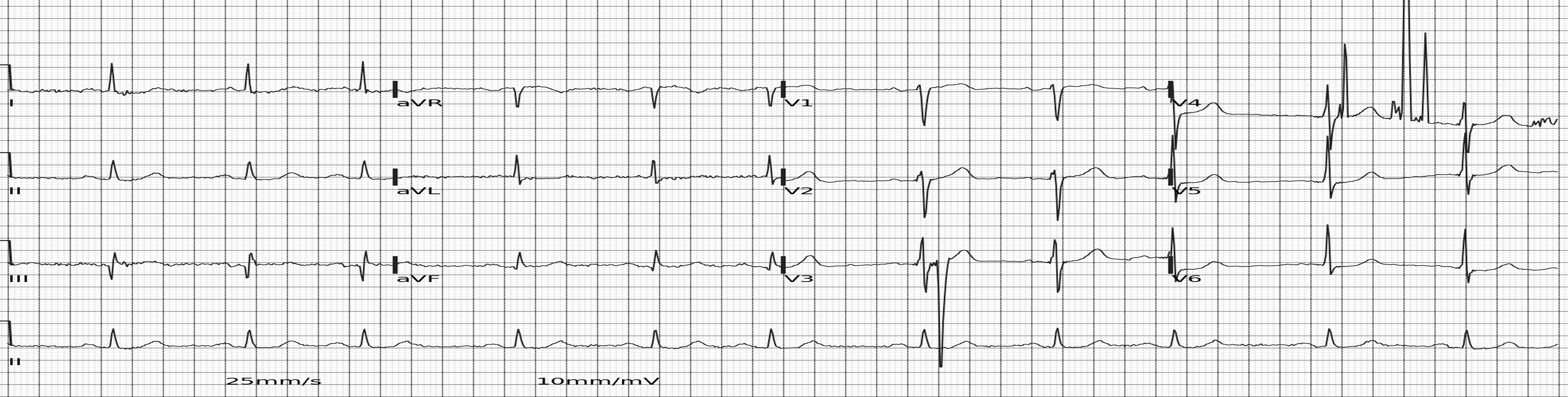\n\n### 2. Prediction Strategy 1\nFeatures from the last and second-to-last blocks of the backbone are used as inputs for numerical prediction. Since the ECG images consist of four vertically stacked data groups, these features are partitioned by height into four segments. These segments are then expanded to four times the input image width.\n\n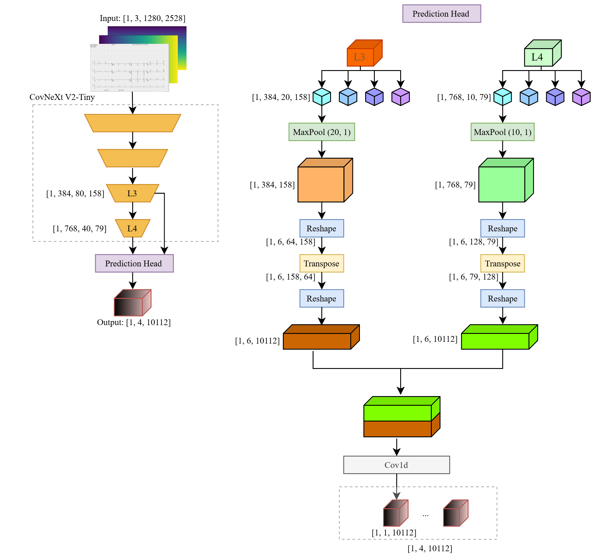\n\n### 3. Prediction Strategy 2\nFeatures from the last block of the backbone are used as inputs for numerical prediction. Given that the ECG images contain four vertically stacked data groups, the features are partitioned by height into four segments. These segments are then expanded to four times the input image width.\n\n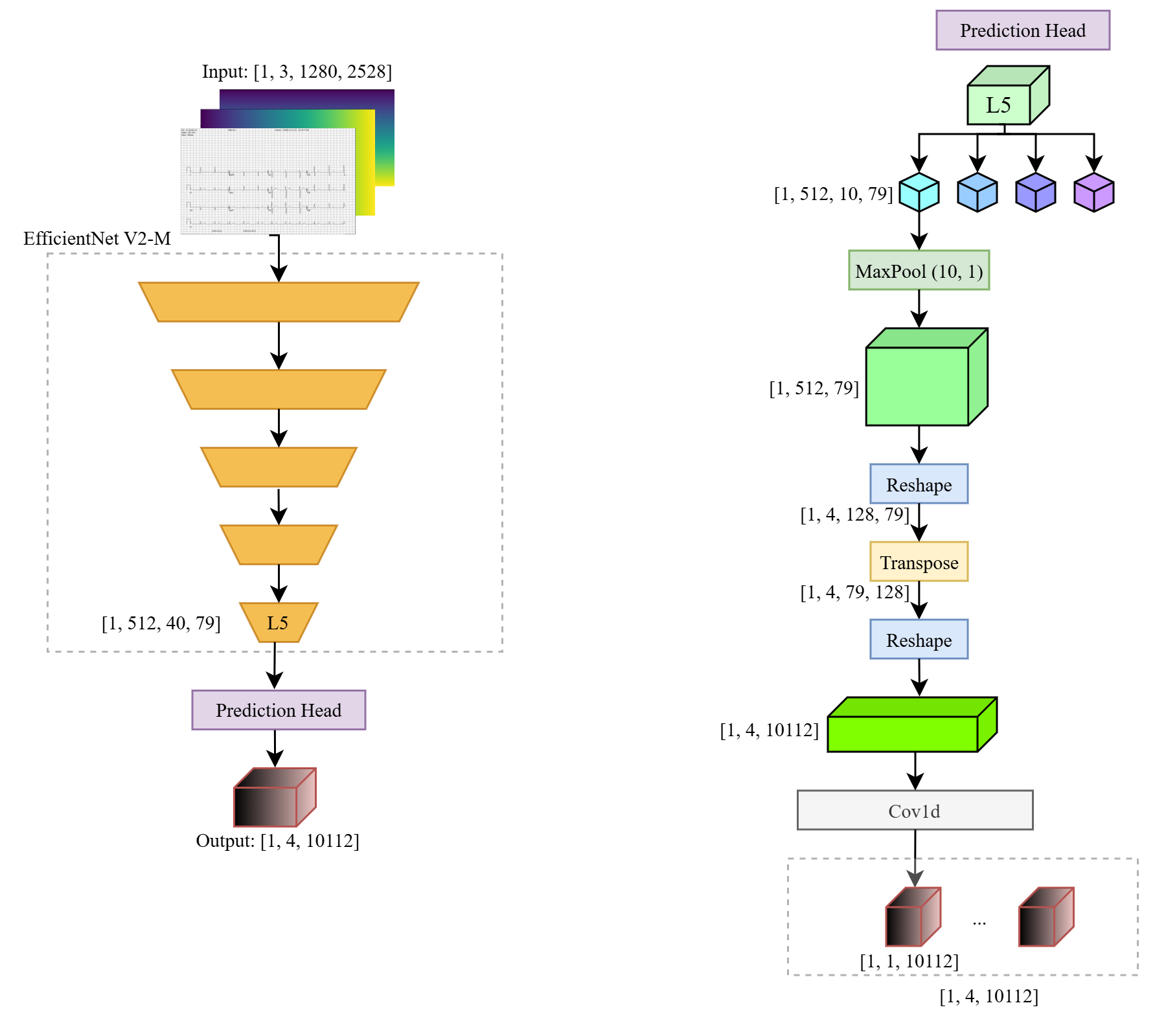\n\n### 4. Prediction Strategy 3\nFeatures from the last block of the backbone are used as the input for numerical prediction. Unlike Strategy 1 and Strategy 2, instead of partitioning features by height, the height dimension is first merged using max pooling. The channels are then split into four segments and expanded to four times the input image width.\n\n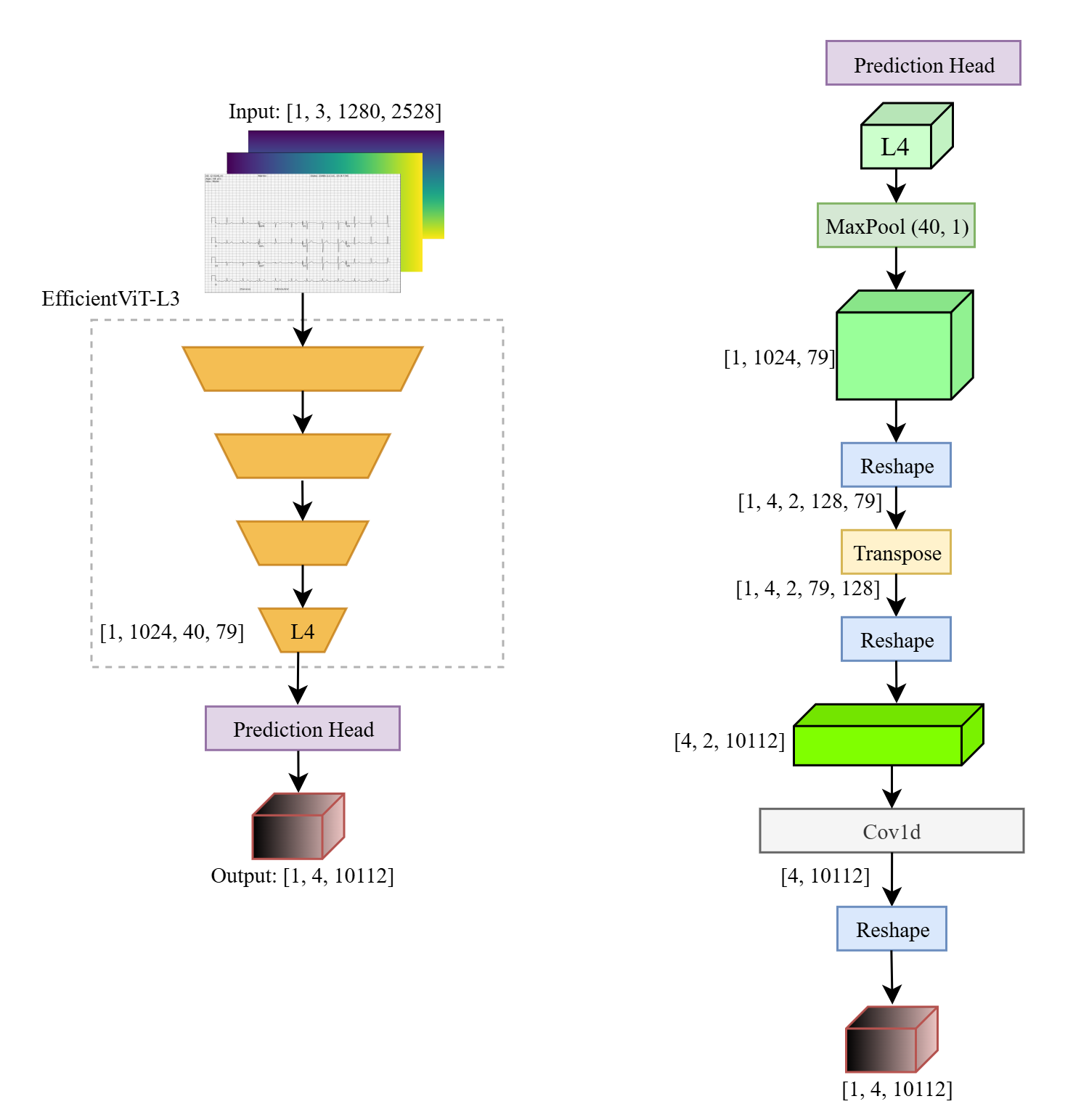\n\n### 5. Post-Processing\nBased on the model output, the middle 10,000, 15,000, or 20,000 outputs are selected and subsequently resampled. Following this, three types of lead blending are performed based on ECG characteristics and Einthoven’s Law to refine the signals\n - Mix the first quarter of the long II with the II\n \n $$II = (II\\times1.35+long II)\\div2.35$$\n\n - Apply 'II = I + III' if np.abs(II-I-III).mean()<0.01\n\n $$I = (I+(II-III)\\times0.6)\\div1.6$$\n \n $$II = (II+(I+III)\\times0.3)\\div1.3$$\n \n $$III = (III+(II-I)\\times0.6)\\div1.6$$\n\n - Apply 'aVR + aVL + aVF = 0' if np.abs(aVR+aVL+aVF).mean()<0.01\n\n $$aVR = (aVR+(-aVL-aVF)\\times0.5)\\div1.5$$\n \n $$aVL = (aVL+(-aVR-aVF)\\times0.5)\\div1.5$$\n \n $$aVF = (aVF+(-aVR-aVL)\\times0.5)\\div1.5$$\n \n### 6. TTA\nA total of three Test-Time Augmentation (TTA) strategies were implemented. These involve gamma adjustments (1.0, 0.9, and 1.1) for brightness control, alongside cropping and resizing of the Stage 1 inputs.\n - Cropping: The Stage 1 inputs were resized to 1560x1248, followed by a center crop of 1440x1152.\n - Resizing: The input resolution for Stage 1 was resized to 1600x1280.\n\n### 6. Training Details\nSmoothL1Loss was used as the loss function, with AdamW as the optimizer and a batch size of 1. The learning rate was set to 1e-4 and managed by a cosine learning rate schedule.\n\n#### Augmentation\nSynthetic blank ECG images were generated to prevent the model from predicting anomalous values when encountering occlusions or noise. Random variations were also applied to the ground truth data to increase diversity. Furthermore, Moiré patterns, flares, and overlaid non-rectified images were introduced to increase training difficulty and enhance model robustness.\n\n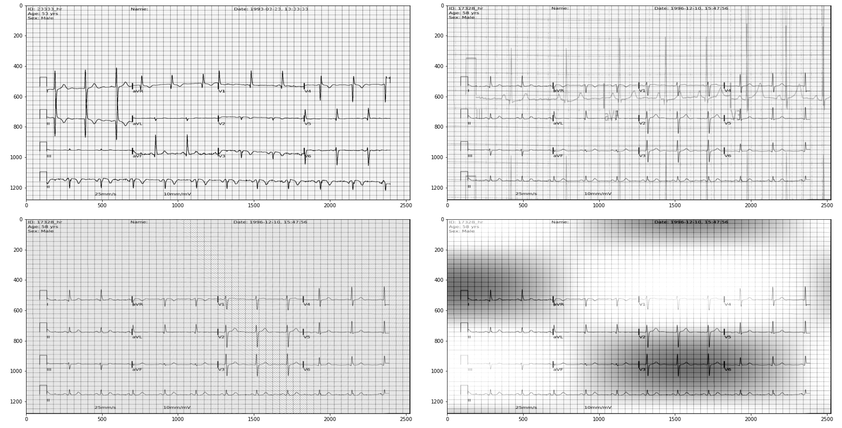\n\n## Results\nA total of ten models were ensembled. For validation, 30 images were selected by taking three segment (0006, 0009, and 0012) from ten image id.\n\nThe implementation of TTA improved overall performance by 0.07, while the Einthoven’s Law-based correction provided an additional 0.06 boost.\n\n| Model | Validation | LB (Private) | Backbone | Input Size | Output Size | Predication Strategy | Ensemble Weight |\n| :---: | :---: | :---: | :---: | :---: | :---: | :---: | :---: |\n| 1 | 26.79 | | convnextv2_tiny | 5056x1280 | 4x20000 | Strategy 1 | 20 |\n| 2 | 26.21 | | convnextv2_base | 2528x1280 | 4x10000 | Strategy 1 | 32 |\n| 3 | 26.50 | | tf_efficientnetv2_m | 5056x1280 | 4x20000 | Strategy 2 | 30 |\n| 4 | 26.03 | | hgnetv2_b6 | 5056x1280 | 4x20000 | Strategy 2 | 11 |\n| 5 | 26.46 | | mambaout_base | 5056x1280 | 4x20000 | Strategy 2 | 8 |\n| 6 | 25.65 | | caformer_m36 | 2528x1280 | 4x10000 | Strategy 2 | 9 |\n| 7 | 26.77 | 22.98 (22.75) | convnextv2_tiny | 5056x1280 | 4x15000 | Strategy 3 | 31 |\n| 8 | 26.56 | | inception_next_small | 5056x1280 | 4x15000 | Strategy 3 | 23 |\n| 9 | 26.76 | | inception_next_base | 5056x1280 | 4x20000 | Strategy 3 | 27 |\n| 10 | 26.78 | | inception_next_base | 5056x1280 | 4x20000 | Strategy 1 | 25 |\n\n### 1. Crossing signal\nTo evaluate model robustness, ECG-Image-Kit was used to select cases where leads overlap or cross each other. Results demonstrate that even in scenarios where Lead V3 and Lead II partially intersect, the model remains capable of generating accurate predictions.\n\n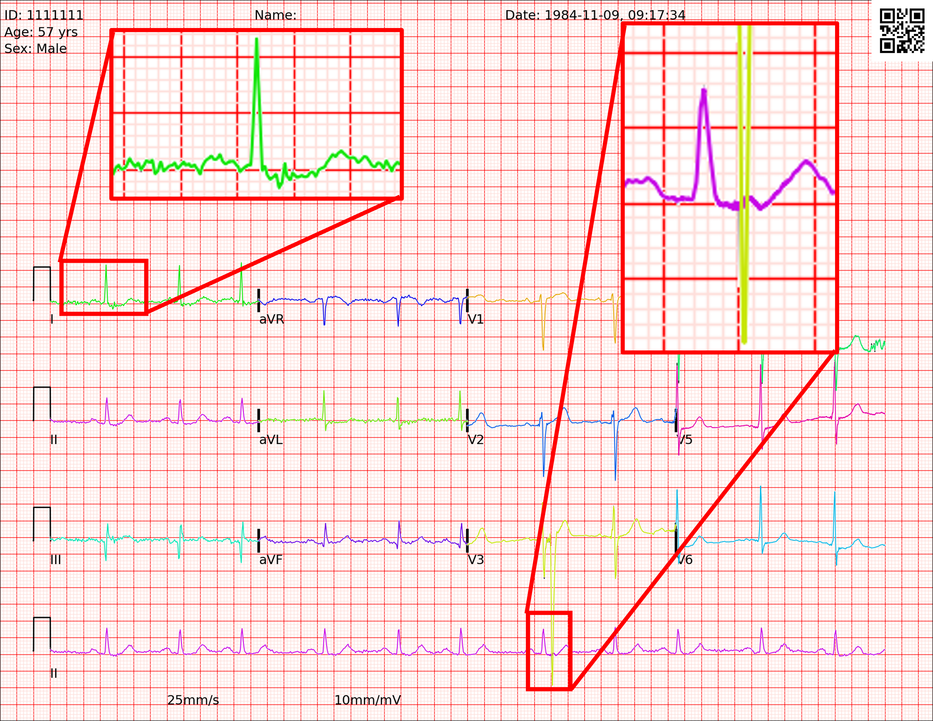\n\n### 2. Resampling\nSNR differences were compared between post-processing using scipy.signal.resample and linear interpolation. (Only test one image at local)\n\n|| Scipy.signal.resample | Linear interpolation |\n| :----: | :----: | :----: |\n|SNR| 23.834 | 22.176 |\n\n### 3. Remapping\nSNR differences were compared between remapping from high-resolution and low-resolution images. (Only test one image at local)\n\n|| Remapping from high resolution | Remapping from low resolution |\n| :----: | :----: | :----: |\n|SNR| 23.834 | 21.267 |\n\n### 4. Rectification\nTwo primary enhancements were implemented for the original rectification method to improve output quality\n1. Grid point positions are calculated using a weighted average from the feature map to preserve floating-point precision.\n2. Surface fitting is utilized to identify and remove outliers, with the resulting gaps filled through interpolation or the regression function itself. This approach ensures smooth image edges and significantly enhances the overall structural integrity of the rectified images.\n\n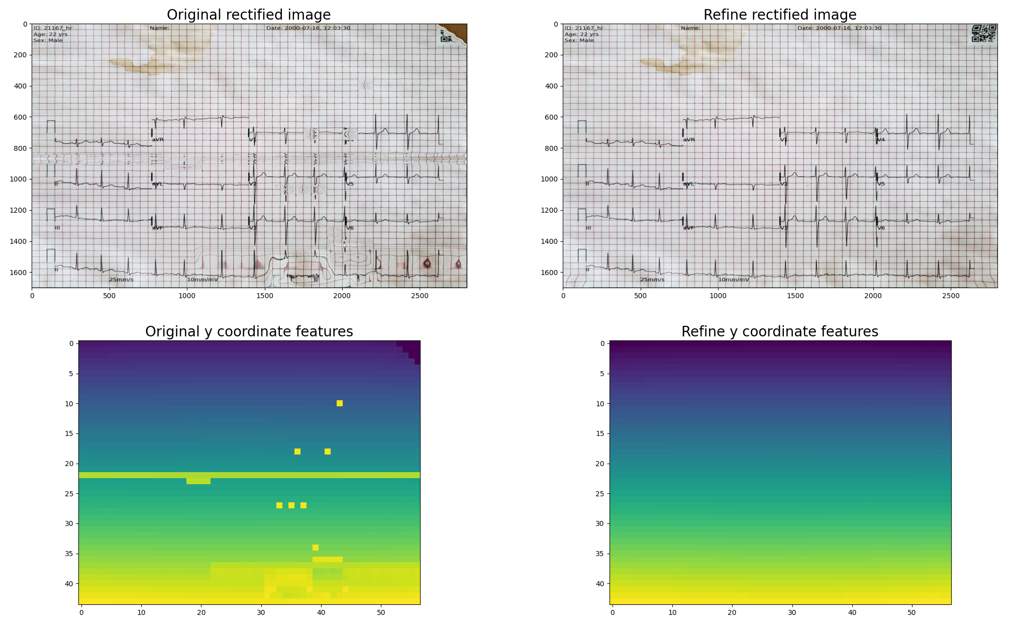\n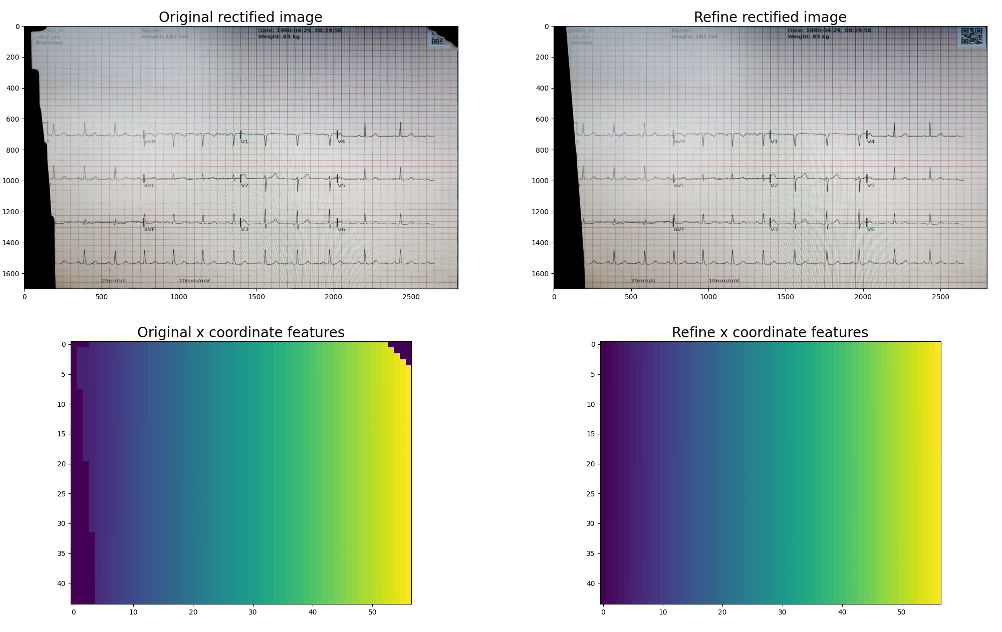\n\n## Other\nImage 3 was generated by scanning Image 1, but we found offset between grid and signal in Image 3 is different from that in Image 1.\n\n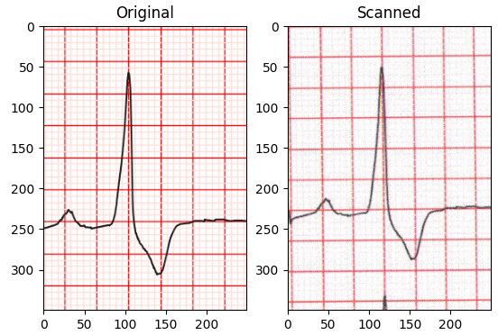", "3395705": "Thanks for the write-up, and congrats to the team on the win 🎉\n\nCan you share the intuition behind the reshape, transpose, reshape operation in the prediction head? If I understand correctly, it looks like this keeps spatial alignment whilst also giving the ability to learn information from adjacent leads?", "3395919": "Thanks, it is for keeping spatial whilst. The output should be [x0c0, x0c1, ... x1c0, x1c1 .....], so we transpose before merge. About what it learns, I am not sure. We think for ever x and lead, the signal value is in proper position of y, and numerous c also take subpixel information into account.", "3396380": "I read in some papers that direct regression of rectification 44x57 is possible. Ie, homography normalised image —> regression net —> 44x57 rectification.", "3396395": "Sure, we tried to regression by normalized image (non-rectified) and got proper score but not competitive. We also try to predict all pixel's original coordinate then apply inverse remap, it is good but also not competitive enough.", "3396721": "Thanks for the reply. When I design my solution, i am very surprised that direct line index prediction (44 and 57 classes) can actually work. The location information encoded in CNN is very rich and precise (or the input is very uniform or repetitive)", "3396825": "Yes, your solution is very impressive, thanks." }, "source": "meta" }