
This solution addresses the PhysioNet challenge of digitizing ECG images—converting printed/photographed ECG recordings back into numerical waveform data. The approach uses a 3-stage deep learning pipeline that progressively transforms raw ECG images into high-fidelity digital waveforms.
\nFinal Public Leaderboard Score: 21.56 SNR\nFinal Private Leaderboard Score: 21.37 SNR
\nECG images from various sources (printed records, mobile phone photos, scans of damaged documents) need to be converted back to digital waveforms. The challenge involves:
\n
Purpose: Detect lead markers and correct image orientation
\n\n\nNote: For this stage, I utilized the pre-trained Stage 0 checkpoint provided in the original baseline.
\n
Purpose: Detect and correct grid distortions
\n\n\nNote: Similar to Stage 0, I used the pre-trained Stage 1 checkpoint from the original baseline.
\n
Purpose: Extract ECG waveforms from rectified images
\nThis is the main prediction stage where most of the innovation lies.
\n
HRNet-W48 Backbone: Maintains high-resolution representations throughout the network via parallel branches, crucial for precise pixel-level waveform prediction
CoordConv Decoder: Injects normalized 2D coordinates at each decoder block, enabling position-aware predictions essential for ECG layout understanding
RGB Skip Connection: Direct connection from input image to prediction head preserves fine spatial details that may be lost in encoder compression
PixelShuffle Upsampling: Memory-efficient learnable upsampling using sub-pixel convolution instead of transposed convolution
GroupNorm: Enables stable training with batch size 1 (necessary for high-resolution 1696×4352 images on limited GPU memory)
The model uses Binary Cross-Entropy (BCE) with positive class weighting for pixel-level supervision:
\nloss = F.binary_cross_entropy_with_logits(\n pixel_logit,\n target_mask,\n pos_weight=10.0 # Handle sparse ECG line pixels\n)\nThis was found to outperform regression-based losses (MSE, SNR) for this task.
\nA comprehensive segment-aware augmentation pipeline was developed to match the diverse training data distribution:
\n| Augmentation | \nProbability | \nPurpose | \n
|---|---|---|
| Perlin Noise | \n85% | \nSimulate scanner noise, paper texture | \n
| Texture Noise | \n70% | \nGrid-like artifacts, scan lines | \n
| Color Jitter | \n80% | \nBrightness, contrast, saturation, hue variation | \n
| Gaussian Noise | \n50% | \nScanner ISO noise | \n
| Gaussian Blur | \n35% | \nLow-quality scans, out-of-focus photos | \n
| Shadow Overlay | \n35% | \nUneven lighting | \n
| Paper Texture | \n30% | \nPhysical paper grain simulation | \n
| JPEG Artifacts | \n30% | \nCompression artifacts | \n
| Horizontal Flip | \n50% | \nData augmentation (with label flip) | \n
The training data contains 12 segment types with distinct characteristics. The augmentation pipeline applies targeted degradations based on segment type:
\n| Segment | \nCharacteristics | \nApplied Augmentations | \n
|---|---|---|
| 0003 | \nStandard color scans | \nBaseline augmentations only | \n
| 0004 | \nBlack & white scans | \nGrayscale conversion + paper tint | \n
| 0005 | \nMobile phone photos | \nVignetting + shadow gradients | \n
| 0006 | \nScreen photos | \nMoiré patterns + screen glare | \n
| 0009 | \nWater-damaged | \nWater stains + color bleeding | \n
| 0010 | \nExtensively damaged | \nFold creases + heavy noise | \n
| 0011, 0012 | \nMoldy scans | \nMold patches + grayscale | \n
To avoid expensive on-the-fly augmentation operations (especially Perlin noise generation), a memory-mapped caching system pre-computes augmentation masks:
\n| Parameter | \nValue | \n
|---|---|
| Batch Size | \n1 (4352×1696 full resolution) | \n
| Optimizer | \nAdamW | \n
| Learning Rate | \n1e-4 | \n
| Weight Decay | \n0.05 | \n
| Epochs | \n80 | \n
| EMA Decay | \n0.999 | \n
| Train/Val Split | \n100/0 (full training set) | \n
| Mixed Precision | \nFP16 (AMP) | \n
| Gradient Checkpointing | \nEnabled for decoder | \n
Horizontal flip TTA improves robustness:
\nA physics-based post-processing step enforces the electrocardiogram constraint:
\nEinthoven's Law: Lead II = Lead I + Lead III
The correction redistributes violation errors across all three limb leads:
\nerror = II - (I + III)\nI_corrected = I + α × error\nIII_corrected = III + α × error\nII_corrected = II - α × error # α = 0.33\nThe 4-strip pixel predictions are converted to waveforms via:
\n\n\nNote: These scores are approximate. Changes were not isolated individually to facilitate faster iteration and save compute costs.
\n
| Configuration | \nPublic LB Score | \n
|---|---|
| Baseline (BCE loss + comprehensive augmentations, 90/10 split) | \n~15.31 | \n
| + High Resolution (1696×4352) | \n~18.22 | \n
| + HRNet-W48 backbone (replacing ResNet) | \n~20.90 | \n
| + 100/0 train/val split (use all training data) | \n~21.01 | \n
| + Horizontal Flip TTA | \n~21.28 | \n
| + Einthoven's Law correction | \n~21.32 | \n
| + RGB Skip + PixelShuffle + Fusion Head | \n~21.56 | \n
Resolution matters: Increasing from standard resolution to 1696×4352 provided the biggest single improvement (~3 SNR)
HRNet superiority: The multi-resolution parallel branches preserve spatial precision better than traditional encoder-decoder architectures
Full training data: With comprehensive augmentation, using 100% of data for training outperformed keeping a validation set
Physics constraints help: Einthoven correction provides consistent small improvements by enforcing known ECG relationships
Training on high-resolution images (1696×4352) with batch size 1 required careful memory management:
\n├── stage0_model.py # Stage 0: Marker detection & normalization\n├── stage1_model.py # Stage 1: Grid detection & rectification\n├── stage2_model.py # Stage 2: Waveform prediction (main model)\n├── predictor_dataset.py # Training data loading & preprocessing\n├── predictor_trainer.py # Training loop with EMA, metrics\n├── augmentations.py # Comprehensive augmentation pipeline\n├── augmentation_cache.py # Memory-mapped augmentation caching\n├── demo-submission.py # End-to-end inference & submission generation\n├── config_predictor.yaml # Training configuration\n└── archive/\n ├── stage0-last.checkpoint.pth # Stage 0 pretrained weights\n └── stage1-last.checkpoint.pth # Stage 1 pretrained weights\nThis solution achieves strong performance on ECG digitization through:
\nHope you enjoyed my writeup. Thanks for reading!
\nThis solution builds upon the excellent work shared by the Kaggle community:
\nThis solution addresses the PhysioNet challenge of digitizing ECG images—converting printed/photographed ECG recordings back into numerical waveform data. The approach uses a 3-stage deep learning pipeline that progressively transforms raw ECG images into high-fidelity digital waveforms.
\nFinal Public Leaderboard Score: 21.56 SNR\nFinal Private Leaderboard Score: 21.37 SNR
\nECG images from various sources (printed records, mobile phone photos, scans of damaged documents) need to be converted back to digital waveforms. The challenge involves:
\n
Purpose: Detect lead markers and correct image orientation
\n\n\nNote: For this stage, I utilized the pre-trained Stage 0 checkpoint provided in the original baseline.
\n
Purpose: Detect and correct grid distortions
\n\n\nNote: Similar to Stage 0, I used the pre-trained Stage 1 checkpoint from the original baseline.
\n
Purpose: Extract ECG waveforms from rectified images
\nThis is the main prediction stage where most of the innovation lies.
\n
HRNet-W48 Backbone: Maintains high-resolution representations throughout the network via parallel branches, crucial for precise pixel-level waveform prediction
CoordConv Decoder: Injects normalized 2D coordinates at each decoder block, enabling position-aware predictions essential for ECG layout understanding
RGB Skip Connection: Direct connection from input image to prediction head preserves fine spatial details that may be lost in encoder compression
PixelShuffle Upsampling: Memory-efficient learnable upsampling using sub-pixel convolution instead of transposed convolution
GroupNorm: Enables stable training with batch size 1 (necessary for high-resolution 1696×4352 images on limited GPU memory)
The model uses Binary Cross-Entropy (BCE) with positive class weighting for pixel-level supervision:
\nloss = F.binary_cross_entropy_with_logits(\n pixel_logit,\n target_mask,\n pos_weight=10.0 # Handle sparse ECG line pixels\n)\nThis was found to outperform regression-based losses (MSE, SNR) for this task.
\nA comprehensive segment-aware augmentation pipeline was developed to match the diverse training data distribution:
\n| Augmentation | \nProbability | \nPurpose | \n
|---|---|---|
| Perlin Noise | \n85% | \nSimulate scanner noise, paper texture | \n
| Texture Noise | \n70% | \nGrid-like artifacts, scan lines | \n
| Color Jitter | \n80% | \nBrightness, contrast, saturation, hue variation | \n
| Gaussian Noise | \n50% | \nScanner ISO noise | \n
| Gaussian Blur | \n35% | \nLow-quality scans, out-of-focus photos | \n
| Shadow Overlay | \n35% | \nUneven lighting | \n
| Paper Texture | \n30% | \nPhysical paper grain simulation | \n
| JPEG Artifacts | \n30% | \nCompression artifacts | \n
| Horizontal Flip | \n50% | \nData augmentation (with label flip) | \n
The training data contains 12 segment types with distinct characteristics. The augmentation pipeline applies targeted degradations based on segment type:
\n| Segment | \nCharacteristics | \nApplied Augmentations | \n
|---|---|---|
| 0003 | \nStandard color scans | \nBaseline augmentations only | \n
| 0004 | \nBlack & white scans | \nGrayscale conversion + paper tint | \n
| 0005 | \nMobile phone photos | \nVignetting + shadow gradients | \n
| 0006 | \nScreen photos | \nMoiré patterns + screen glare | \n
| 0009 | \nWater-damaged | \nWater stains + color bleeding | \n
| 0010 | \nExtensively damaged | \nFold creases + heavy noise | \n
| 0011, 0012 | \nMoldy scans | \nMold patches + grayscale | \n
To avoid expensive on-the-fly augmentation operations (especially Perlin noise generation), a memory-mapped caching system pre-computes augmentation masks:
\n| Parameter | \nValue | \n
|---|---|
| Batch Size | \n1 (4352×1696 full resolution) | \n
| Optimizer | \nAdamW | \n
| Learning Rate | \n1e-4 | \n
| Weight Decay | \n0.05 | \n
| Epochs | \n80 | \n
| EMA Decay | \n0.999 | \n
| Train/Val Split | \n100/0 (full training set) | \n
| Mixed Precision | \nFP16 (AMP) | \n
| Gradient Checkpointing | \nEnabled for decoder | \n
Horizontal flip TTA improves robustness:
\nA physics-based post-processing step enforces the electrocardiogram constraint:
\nEinthoven's Law: Lead II = Lead I + Lead III
The correction redistributes violation errors across all three limb leads:
\nerror = II - (I + III)\nI_corrected = I + α × error\nIII_corrected = III + α × error\nII_corrected = II - α × error # α = 0.33\nThe 4-strip pixel predictions are converted to waveforms via:
\n\n\nNote: These scores are approximate. Changes were not isolated individually to facilitate faster iteration and save compute costs.
\n
| Configuration | \nPublic LB Score | \n
|---|---|
| Baseline (BCE loss + comprehensive augmentations, 90/10 split) | \n~15.31 | \n
| + High Resolution (1696×4352) | \n~18.22 | \n
| + HRNet-W48 backbone (replacing ResNet) | \n~20.90 | \n
| + 100/0 train/val split (use all training data) | \n~21.01 | \n
| + Horizontal Flip TTA | \n~21.28 | \n
| + Einthoven's Law correction | \n~21.32 | \n
| + RGB Skip + PixelShuffle + Fusion Head | \n~21.56 | \n
Resolution matters: Increasing from standard resolution to 1696×4352 provided the biggest single improvement (~3 SNR)
HRNet superiority: The multi-resolution parallel branches preserve spatial precision better than traditional encoder-decoder architectures
Full training data: With comprehensive augmentation, using 100% of data for training outperformed keeping a validation set
Physics constraints help: Einthoven correction provides consistent small improvements by enforcing known ECG relationships
Training on high-resolution images (1696×4352) with batch size 1 required careful memory management:
\n├── stage0_model.py # Stage 0: Marker detection & normalization\n├── stage1_model.py # Stage 1: Grid detection & rectification\n├── stage2_model.py # Stage 2: Waveform prediction (main model)\n├── predictor_dataset.py # Training data loading & preprocessing\n├── predictor_trainer.py # Training loop with EMA, metrics\n├── augmentations.py # Comprehensive augmentation pipeline\n├── augmentation_cache.py # Memory-mapped augmentation caching\n├── demo-submission.py # End-to-end inference & submission generation\n├── config_predictor.yaml # Training configuration\n└── archive/\n ├── stage0-last.checkpoint.pth # Stage 0 pretrained weights\n └── stage1-last.checkpoint.pth # Stage 1 pretrained weights\nThis solution achieves strong performance on ECG digitization through:
\nHope you enjoyed my writeup. Thanks for reading!
\nThis solution builds upon the excellent work shared by the Kaggle community:
\nThank you so much for sharing such a detailed and thorough solution! When I was going through your code and solution, I noticed that you use all types of training images after rectification as the input for Stage 2 during training. However, in my tests, the rectified non-0001 type images are not perfectly aligned with the GT signals. I wonder how you addressed this issue, or if I have any misunderstanding of your solution.
", "rawMarkdown": "Thank you so much for sharing such a detailed and thorough solution! When I was going through your code and solution, I noticed that you use all types of training images after rectification as the input for Stage 2 during training. However, in my tests, the rectified non-0001 type images are not perfectly aligned with the GT signals. I wonder how you addressed this issue, or if I have any misunderstanding of your solution.", "votes": null }, { "id": "3395576", "postDate": "01/23/2026 08:55:46", "content": "That is a great observation! I also noticed that due to rectification errors in stage 0 and 1, the GT signals are not always perfectly aligned with what we see visually (mostly due to horizontal misalignment).
\n
I do agree that this creates some training confusion. However, I believe that this actually does not significantly hurt performance for the following reasons:
\nThe key distinction is where and how the timespan constraint is applied:
\n# Hypothetical: Model architecture prevents predictions outside timespan\nclass HardConstrainedModel:\n def forward(self, batch):\n x = batch['image']\n features = self.encoder(x)\n output = torch.zeros(B, 4, H, W)\n # Only allow decoder to predict in specific columns\n output[:, :, :, 235:4161] = self.decoder(features)[:, :, :, 235:4161]\n return {'pixel_logit': output} # Forced zeros outside [235, 4161]\nThis would completely prevent the model from learning waveform features outside [235-4161].
\nModel architecture (stage2_model.py):
def forward(self, batch, L=None):\n image = batch['image'] # (B, 3, H, W)\n # ... encoder + decoder ...\n pixel_logit = self.pixel_out(last) # (B, 4, H, W) - FULL width prediction\n return {'pixel_logit': pixel_logit} # No spatial masking\nTraining (predictor_trainer.py):
# Loss is computed on FULL image\npixel_loss = F.binary_cross_entropy_with_logits(\n pixel_logit, # (B, 4, H, W=4352) - all columns\n pixel_target, # (B, 4, H, W=4352) - GT drawn at [235, 4161]\n pos_weight=pos_weight,\n)\n# Model learns to activate [235-4161] due to GT distribution,\n# but architecture doesn't prevent activations elsewhere\nInference (predictor_trainer.py):
def _predict_waveform(self, image_u8, target_len):\n out = self.model(batch)\n pixel_logit = out['pixel_logit'] # (B, 4, H, W) - full width\n\n # Convert ALL columns to y-positions\n y_hat = pixel_logits_to_y(pixel_logit, ...) # (B, 4, W)\n\n # Crop to timespan AFTER conversion (post-processing, not architectural)\n y_hat = y_hat[..., self.t0:self.t1] # (B, 4, 3926)\n\n mv_hat = y_to_mv(y_hat, ...)\n return mv_hat\nFor a misaligned sample where the waveform appears at columns [200-4126] instead of [235-4161]:
\nWith Hard Prior:
\nWith Soft Prior:
\nThe GT is drawn into [235-4161], but the model sees and processes the entire image during training. Visual features from misaligned regions still contribute to learning through the convolutional receptive field.
\nThe system degrades gracefully rather than failing catastrophically.
\nThis design choice accepts some label noise from imperfect rectifications in exchange for:
\nThank you so much for your patient explanation. Your answer has cleared up my confusion. I have one more question: when constructing the training data, did you manually check and exclude some severely misaligned samples, or did you use all the rectified images directly?
", "rawMarkdown": "Thank you so much for your patient explanation. Your answer has cleared up my confusion. I have one more question: when constructing the training data, did you manually check and exclude some severely misaligned samples, or did you use all the rectified images directly?", "votes": null }, { "id": "3395753", "postDate": "01/23/2026 15:57:51", "content": "I used all rectified images directly without manual filtering or exclusion.
\nI generally avoid removing data due to fear of information loss. In my experience, severely misaligned samples are quite rare - the vast majority of rectifications from Stage 0+1 are reasonably accurate. The few badly misaligned samples act as noise in the training set, but with enough well-aligned data, the model naturally learns to filter out these outliers and converge to the correct visual features.
\nThe benefits of keeping all data (more diverse training samples, better coverage of edge cases) outweighed the cost of a small amount of label noise from misalignments.
", "rawMarkdown": "I used all rectified images directly without manual filtering or exclusion.\n\nI generally avoid removing data due to fear of information loss. In my experience, severely misaligned samples are quite rare - the vast majority of rectifications from Stage 0+1 are reasonably accurate. The few badly misaligned samples act as noise in the training set, but with enough well-aligned data, the model naturally learns to filter out these outliers and converge to the correct visual features.\n\nThe benefits of keeping all data (more diverse training samples, better coverage of edge cases) outweighed the cost of a small amount of label noise from misalignments.", "votes": null }, { "id": "3395806", "postDate": "01/23/2026 17:16:58", "content": "Regarding the alignment issue:\nI think teams that use direct regression (i.e., mapping from images to values) will not have this issue. This is because crooked lines provide cues for the network to adjust misaligned pixel locations and still predict the correct values.
", "rawMarkdown": "Regarding the alignment issue:\nI think teams that use direct regression (i.e., mapping from images to values) will not have this issue. This is because crooked lines provide cues for the network to adjust misaligned pixel locations and still predict the correct values.", "votes": null }, { "id": "3395917", "postDate": "01/23/2026 23:44:16", "content": "I think so too. And thanks again for your great work, it helps us a lot.😃
", "rawMarkdown": "I think so too. And thanks again for your great work, it helps us a lot.😃", "votes": null } ], "comments": [ { "id": 3395554, "author_name": "xie233", "author_url": "", "post_date": "01/23/2026 07:45:49", "content": "Thank you so much for sharing such a detailed and thorough solution! When I was going through your code and solution, I noticed that you use all types of training images after rectification as the input for Stage 2 during training. However, in my tests, the rectified non-0001 type images are not perfectly aligned with the GT signals. I wonder how you addressed this issue, or if I have any misunderstanding of your solution.
", "votes": null, "replies": [ { "id": 3395576, "author_name": "sshiyu", "author_url": "", "post_date": "01/23/2026 08:55:46", "content": "That is a great observation! I also noticed that due to rectification errors in stage 0 and 1, the GT signals are not always perfectly aligned with what we see visually (mostly due to horizontal misalignment).
\n
I do agree that this creates some training confusion. However, I believe that this actually does not significantly hurt performance for the following reasons:
\nThe key distinction is where and how the timespan constraint is applied:
\n# Hypothetical: Model architecture prevents predictions outside timespan\nclass HardConstrainedModel:\n def forward(self, batch):\n x = batch['image']\n features = self.encoder(x)\n output = torch.zeros(B, 4, H, W)\n # Only allow decoder to predict in specific columns\n output[:, :, :, 235:4161] = self.decoder(features)[:, :, :, 235:4161]\n return {'pixel_logit': output} # Forced zeros outside [235, 4161]\nThis would completely prevent the model from learning waveform features outside [235-4161].
\nModel architecture (stage2_model.py):
def forward(self, batch, L=None):\n image = batch['image'] # (B, 3, H, W)\n # ... encoder + decoder ...\n pixel_logit = self.pixel_out(last) # (B, 4, H, W) - FULL width prediction\n return {'pixel_logit': pixel_logit} # No spatial masking\nTraining (predictor_trainer.py):
# Loss is computed on FULL image\npixel_loss = F.binary_cross_entropy_with_logits(\n pixel_logit, # (B, 4, H, W=4352) - all columns\n pixel_target, # (B, 4, H, W=4352) - GT drawn at [235, 4161]\n pos_weight=pos_weight,\n)\n# Model learns to activate [235-4161] due to GT distribution,\n# but architecture doesn't prevent activations elsewhere\nInference (predictor_trainer.py):
def _predict_waveform(self, image_u8, target_len):\n out = self.model(batch)\n pixel_logit = out['pixel_logit'] # (B, 4, H, W) - full width\n\n # Convert ALL columns to y-positions\n y_hat = pixel_logits_to_y(pixel_logit, ...) # (B, 4, W)\n\n # Crop to timespan AFTER conversion (post-processing, not architectural)\n y_hat = y_hat[..., self.t0:self.t1] # (B, 4, 3926)\n\n mv_hat = y_to_mv(y_hat, ...)\n return mv_hat\nFor a misaligned sample where the waveform appears at columns [200-4126] instead of [235-4161]:
\nWith Hard Prior:
\nWith Soft Prior:
\nThe GT is drawn into [235-4161], but the model sees and processes the entire image during training. Visual features from misaligned regions still contribute to learning through the convolutional receptive field.
\nThe system degrades gracefully rather than failing catastrophically.
\nThis design choice accepts some label noise from imperfect rectifications in exchange for:
\nThank you so much for your patient explanation. Your answer has cleared up my confusion. I have one more question: when constructing the training data, did you manually check and exclude some severely misaligned samples, or did you use all the rectified images directly?
", "votes": null, "replies": [ { "id": 3395753, "author_name": "sshiyu", "author_url": "", "post_date": "01/23/2026 15:57:51", "content": "I used all rectified images directly without manual filtering or exclusion.
\nI generally avoid removing data due to fear of information loss. In my experience, severely misaligned samples are quite rare - the vast majority of rectifications from Stage 0+1 are reasonably accurate. The few badly misaligned samples act as noise in the training set, but with enough well-aligned data, the model naturally learns to filter out these outliers and converge to the correct visual features.
\nThe benefits of keeping all data (more diverse training samples, better coverage of edge cases) outweighed the cost of a small amount of label noise from misalignments.
", "votes": null, "replies": [] } ] } ] } ] }, { "id": 3395806, "author_name": "hengck23", "author_url": "", "post_date": "01/23/2026 17:16:58", "content": "Regarding the alignment issue:\nI think teams that use direct regression (i.e., mapping from images to values) will not have this issue. This is because crooked lines provide cues for the network to adjust misaligned pixel locations and still predict the correct values.
", "votes": null, "replies": [ { "id": 3395917, "author_name": "outrunner", "author_url": "", "post_date": "01/23/2026 23:44:16", "content": "I think so too. And thanks again for your great work, it helps us a lot.😃
", "votes": null, "replies": [] } ] } ], "raw_markdown_by_id": { "3395469": "# PhysioNet ECG Digitization Challenge - Solution Writeup\n\n## Overview\nThis solution addresses the PhysioNet challenge of digitizing ECG images—converting printed/photographed ECG recordings back into numerical waveform data. The approach uses a **3-stage deep learning pipeline** that progressively transforms raw ECG images into high-fidelity digital waveforms.\n\n**Final Public Leaderboard Score: 21.56 SNR**\n**Final Private Leaderboard Score: 21.37 SNR**\n\n---\n\n## Problem Statement\n\nECG images from various sources (printed records, mobile phone photos, scans of damaged documents) need to be converted back to digital waveforms. The challenge involves:\n\n1. **Diverse image sources**: High-quality prints, mobile photos, screen captures, damaged/moldy documents\n2. **Geometric distortions**: Perspective warps, rotations, varying aspect ratios\n3. **Visual degradations**: Water stains, fold creases, mold, low resolution, compression artifacts\n4. **Layout parsing**: Standard 4-strip ECG layout with 12 leads arranged in specific positions\n\n---\n## Solution Architecture\n\n### Three-Stage Pipeline\n\n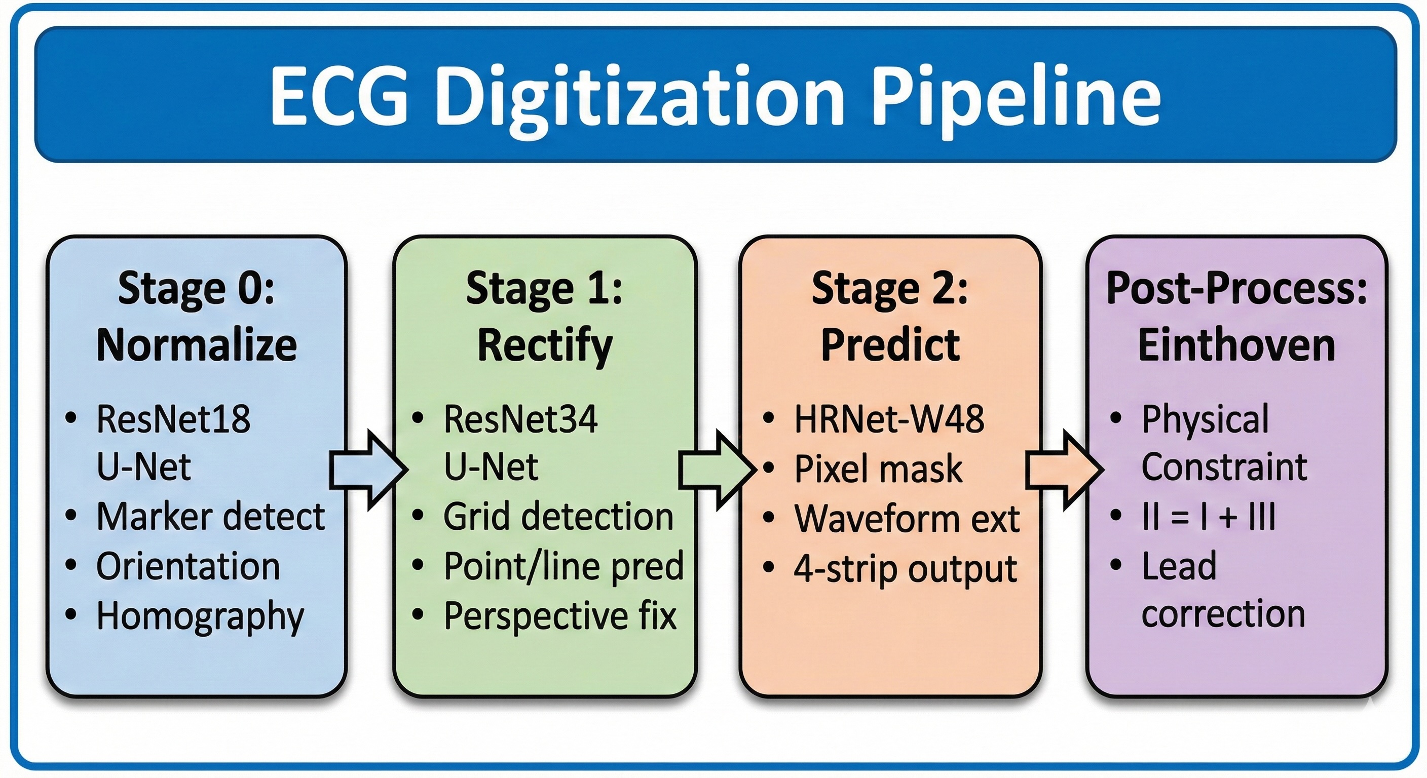\n\n### Stage 0: Normalization\n\n**Purpose**: Detect lead markers and correct image orientation\n\n- **Architecture**: ResNet18 encoder + U-Net decoder\n- **Outputs**: \n - Lead marker segmentation (13 leads + background)\n - Image orientation classification (8 orientations)\n- **Processing**: Applies homography to normalize image to canonical size (3024×4032)\n\n> **Note**: For this stage, I utilized the pre-trained Stage 0 checkpoint provided in the [original baseline](https://www.kaggle.com/code/hengck23/demo-submission).\n\n### Stage 1: Rectification\n\n**Purpose**: Detect and correct grid distortions\n\n- **Architecture**: ResNet34 encoder + U-Net decoder \n- **Outputs**:\n - Grid point detection (keypoints for perspective correction)\n - Horizontal line classification (44 classes)\n - Vertical line classification (57 classes)\n- **Processing**: Uses detected grid points to apply perspective transformation, producing a perfectly aligned rectified image\n\n> **Note**: Similar to Stage 0, I used the pre-trained Stage 1 checkpoint from the [original baseline](https://www.kaggle.com/code/hengck23/demo-submission).\n\n### Stage 2: Waveform Prediction\n\n**Purpose**: Extract ECG waveforms from rectified images\n\nThis is the main prediction stage where most of the innovation lies.\n\n#### Model Architecture\n\n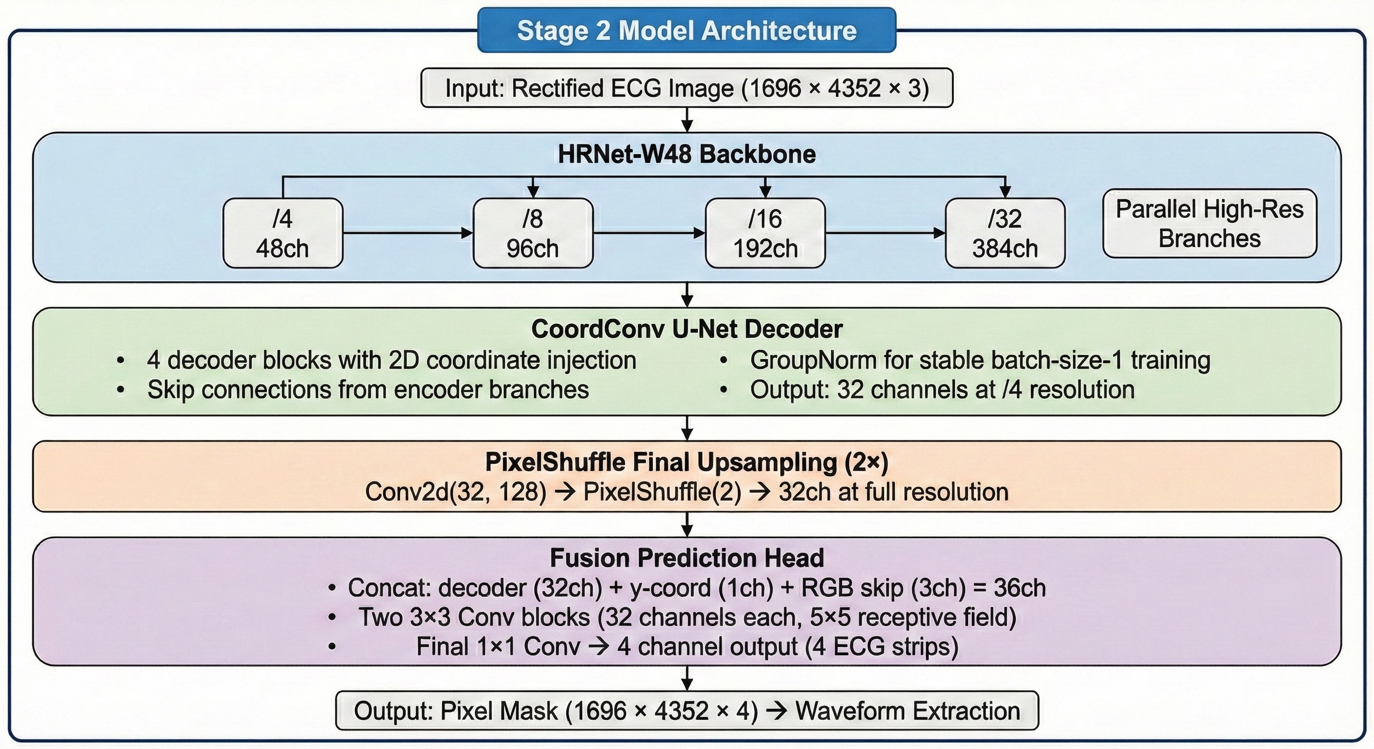\n\n#### Key Design Decisions\n\n1. **HRNet-W48 Backbone**: Maintains high-resolution representations throughout the network via parallel branches, crucial for precise pixel-level waveform prediction\n\n2. **CoordConv Decoder**: Injects normalized 2D coordinates at each decoder block, enabling position-aware predictions essential for ECG layout understanding\n\n3. **RGB Skip Connection**: Direct connection from input image to prediction head preserves fine spatial details that may be lost in encoder compression\n\n4. **PixelShuffle Upsampling**: Memory-efficient learnable upsampling using sub-pixel convolution instead of transposed convolution\n\n5. **GroupNorm**: Enables stable training with batch size 1 (necessary for high-resolution 1696×4352 images on limited GPU memory)\n\n---\n\n## Training Strategy\n\n### Loss Function\n\nThe model uses **Binary Cross-Entropy (BCE) with positive class weighting** for pixel-level supervision:\n\n```python\nloss = F.binary_cross_entropy_with_logits(\n pixel_logit,\n target_mask,\n pos_weight=10.0 # Handle sparse ECG line pixels\n)\n```\n\nThis was found to outperform regression-based losses (MSE, SNR) for this task.\n\n### Data Augmentation\n\nA comprehensive **segment-aware augmentation pipeline** was developed to match the diverse training data distribution:\n\n#### Universal Augmentations\n| Augmentation | Probability | Purpose |\n|-------------|-------------|---------|\n| Perlin Noise | 85% | Simulate scanner noise, paper texture |\n| Texture Noise | 70% | Grid-like artifacts, scan lines |\n| Color Jitter | 80% | Brightness, contrast, saturation, hue variation |\n| Gaussian Noise | 50% | Scanner ISO noise |\n| Gaussian Blur | 35% | Low-quality scans, out-of-focus photos |\n| Shadow Overlay | 35% | Uneven lighting |\n| Paper Texture | 30% | Physical paper grain simulation |\n| JPEG Artifacts | 30% | Compression artifacts |\n| Horizontal Flip | 50% | Data augmentation (with label flip) |\n\n#### Segment-Specific Augmentations\n\nThe training data contains 12 segment types with distinct characteristics. The augmentation pipeline applies targeted degradations based on segment type:\n\n| Segment | Characteristics | Applied Augmentations |\n|---------|-----------------|----------------------|\n| 0003 | Standard color scans | Baseline augmentations only |\n| 0004 | Black & white scans | Grayscale conversion + paper tint |\n| 0005 | Mobile phone photos | Vignetting + shadow gradients |\n| 0006 | Screen photos | Moiré patterns + screen glare |\n| 0009 | Water-damaged | Water stains + color bleeding |\n| 0010 | Extensively damaged | Fold creases + heavy noise |\n| 0011, 0012 | Moldy scans | Mold patches + grayscale |\n\n#### Augmentation Caching\n\nTo avoid expensive on-the-fly augmentation operations (especially Perlin noise generation), a **memory-mapped caching system** pre-computes augmentation masks:\n\n- Perlin noise cache: 512 pre-computed noise maps\n- Texture cache: 256 patterns\n- Shadow/vignette cache: 256 gradient patterns\n\n### Training Configuration\n\n| Parameter | Value |\n|-----------|-------|\n| Batch Size | 1 (4352×1696 full resolution) |\n| Optimizer | AdamW |\n| Learning Rate | 1e-4 |\n| Weight Decay | 0.05 |\n| Epochs | 80 |\n| EMA Decay | 0.999 |\n| Train/Val Split | 100/0 (full training set) |\n| Mixed Precision | FP16 (AMP) |\n| Gradient Checkpointing | Enabled for decoder |\n\n---\n\n## Inference Pipeline\n\n### Test-Time Augmentation (TTA)\n\nHorizontal flip TTA improves robustness:\n\n1. Predict on original image\n2. Horizontally flip input image\n3. Predict on flipped image\n4. Flip prediction back to original orientation\n5. Average both predictions\n\n### Einthoven's Law Correction\n\nA physics-based post-processing step enforces the electrocardiogram constraint:\n\n**Einthoven's Law**: `Lead II = Lead I + Lead III`\n\nThe correction redistributes violation errors across all three limb leads:\n\n```python\nerror = II - (I + III)\nI_corrected = I + α × error\nIII_corrected = III + α × error\nII_corrected = II - α × error # α = 0.33\n```\n\n### Waveform Extraction\n\nThe 4-strip pixel predictions are converted to waveforms via:\n\n1. Apply softmax on y-dimension to get probability distributions\n2. Compute weighted centroid (argmax or soft-argmax) for each x-column\n3. Convert pixel coordinates to mV using calibration parameters\n4. Split each strip into constituent leads based on temporal layout\n5. Resample to target sample lengths specified in test.csv\n\n---\n\n## Ablation Studies\n\n> **Note**: These scores are approximate. Changes were not isolated individually to facilitate faster iteration and save compute costs.\n\n| Configuration | Public LB Score |\n|---------------|-----------------|\n| Baseline (BCE loss + comprehensive augmentations, 90/10 split) | ~15.31 |\n| + High Resolution (1696×4352) | ~18.22 |\n| + HRNet-W48 backbone (replacing ResNet) | ~20.90 |\n| + 100/0 train/val split (use all training data) | ~21.01 |\n| + Horizontal Flip TTA | ~21.28 |\n| + Einthoven's Law correction | ~21.32 |\n| + RGB Skip + PixelShuffle + Fusion Head | ~21.56 |\n\n### Key Insights\n\n1. **Resolution matters**: Increasing from standard resolution to 1696×4352 provided the biggest single improvement (~3 SNR)\n\n2. **HRNet superiority**: The multi-resolution parallel branches preserve spatial precision better than traditional encoder-decoder architectures\n\n3. **Full training data**: With comprehensive augmentation, using 100% of data for training outperformed keeping a validation set\n\n4. **Physics constraints help**: Einthoven correction provides consistent small improvements by enforcing known ECG relationships\n\n---\n\n## Technical Implementation Details\n\n### Memory Optimization\n\nTraining on high-resolution images (1696×4352) with batch size 1 required careful memory management:\n\n- **Gradient Checkpointing**: Enabled for decoder blocks to trade compute for memory\n- **GroupNorm**: Used instead of BatchNorm for stable single-sample training\n- **PixelShuffle**: Used instead of ConvTranspose2d for 2× upsampling (more memory efficient)\n- **Mixed Precision (FP16)**: Enabled via PyTorch AMP\n\n### Distributed Training\n\n- DDP (Distributed Data Parallel) support for multi-GPU training\n- Per-worker augmentation cache to avoid contention\n- Memory-mapped cache files shared across workers\n\n---\n\n## Repository Structure\n\n```\n├── stage0_model.py # Stage 0: Marker detection & normalization\n├── stage1_model.py # Stage 1: Grid detection & rectification\n├── stage2_model.py # Stage 2: Waveform prediction (main model)\n├── predictor_dataset.py # Training data loading & preprocessing\n├── predictor_trainer.py # Training loop with EMA, metrics\n├── augmentations.py # Comprehensive augmentation pipeline\n├── augmentation_cache.py # Memory-mapped augmentation caching\n├── demo-submission.py # End-to-end inference & submission generation\n├── config_predictor.yaml # Training configuration\n└── archive/\n ├── stage0-last.checkpoint.pth # Stage 0 pretrained weights\n └── stage1-last.checkpoint.pth # Stage 1 pretrained weights\n```\n\n---\n\n## Code\n\n- **GitHub Repository**: [starrynites/PhysioNet_Digitization_of_ECG_Images](https://github.com/starrynites/PhysioNet_Digitization_of_ECG_Images)\n- **Kaggle Inference Notebook**: [sshiyu/physionet-final-submission](https://www.kaggle.com/code/sshiyu/physionet-final-submission)\n\n## Conclusion\n\nThis solution achieves strong performance on ECG digitization through:\n\n1. **Robust preprocessing**: Stage 0+1 pipeline handles diverse image sources and geometric distortions\n2. **High-resolution prediction**: Full-resolution HRNet enables precise pixel-level waveform detection\n3. **Comprehensive augmentation**: Segment-aware degradation simulation improves generalization\n4. **Physics-informed post-processing**: Einthoven correction enforces known ECG constraints\n5. **Efficient architecture**: RGB skip connection + PixelShuffle fusion preserves fine details while maintaining training efficiency\n\nHope you enjoyed my writeup. Thanks for reading!\n\n---\n\n## Acknowledgements\n\nThis solution builds upon the excellent work shared by the Kaggle community:\n\n- [hengck23/demo-submission](https://www.kaggle.com/code/hengck23/demo-submission) — Original low resolution baseline\n- [wasupandceacar/physio-v2-3-public](https://www.kaggle.com/code/wasupandceacar/physio-v2-3-public) — High resolution baseline reference\n- [tonylica/physionet-ecg-streamlined-inference](https://www.kaggle.com/code/tonylica/physionet-ecg-streamlined-inference) — Einthoven's law correction idea\n\n### References\n\n- Shivashankara KK, Deepanshi, Shervedani AM, Reyna MA, Clifford GD, Sameni R. ECG-Image-Kit: a synthetic image generation toolbox to facilitate deep learning-based electrocardiogram digitization. Physiological Measurement 2024; 45:055019. DOI: 10.1088/1361-6579/ad4954\n- Reyna MA, Deepanshi, Weigle J, Koscova Z, Campbell K, Shivashankara KK, Saghafi S, Nikookar S, Motie-Shirazi M, Kiarashi Y, Seyedi S, Hassannia M, Bjørnstad AM, Stenhede E, Ranjbar A, Clifford GD, and Sameni R. ECG-Image-Database: A dataset of ECG images with real-world imaging and scanning artifacts; a foundation for computerized ECG image digitization and analysis, 2024. DOI: 10.48550/arXiv.2409.16612.\n- Reyna MA, Deepanshi, Weigle J, Koscova Z, Campbell K, Seyedi S, Elola A, Bahrami Rad A, Shah AJ, Bhatia NK, Clifford GD, Sameni R. Digitization and Classification of ECG Images: The George B. Moody PhysioNet Challenge 2024; Computing in Cardiology 2024; 51: 1-4.\n- Matthew A. Reyna, Deepanshi, James Weigle, Zuzana Koscova, Kiersten Campbell, Salman Seyedi, Andoni Elola, Ali Bahrami Rad, Amit J Shah, Neal K. Bhatia, Yao Yan, Sohier Dane, Addison Howard, Gari D. Clifford, and Reza Sameni. PhysioNet - Digitization of ECG Images. https://kaggle.com/competitions/physionet-ecg-image-digitization, 2025. Kaggle.\n\n---", "3395554": "Thank you so much for sharing such a detailed and thorough solution! When I was going through your code and solution, I noticed that you use all types of training images after rectification as the input for Stage 2 during training. However, in my tests, the rectified non-0001 type images are not perfectly aligned with the GT signals. I wonder how you addressed this issue, or if I have any misunderstanding of your solution.", "3395576": "That is a great observation! I also noticed that due to rectification errors in stage 0 and 1, the GT signals are not always perfectly aligned with what we see visually (mostly due to horizontal misalignment).\n\n\n\nI do agree that this creates some training confusion. However, I believe that this actually does not significantly hurt performance for the following reasons:\n\n1. **Most samples are reasonably well-aligned** - Stage 1 rectification works well for the majority of images\n2. **The spatial prior is \"soft\" rather than \"hard\"** - the model can adapt to misalignments\n\n## Soft vs Hard Spatial Prior\n\nThe key distinction is **where and how** the timespan constraint is applied:\n\n### Hard Spatial Prior (NOT what I do)\n\n```python\n# Hypothetical: Model architecture prevents predictions outside timespan\nclass HardConstrainedModel:\n def forward(self, batch):\n x = batch['image']\n features = self.encoder(x)\n output = torch.zeros(B, 4, H, W)\n # Only allow decoder to predict in specific columns\n output[:, :, :, 235:4161] = self.decoder(features)[:, :, :, 235:4161]\n return {'pixel_logit': output} # Forced zeros outside [235, 4161]\n```\n\nThis would completely prevent the model from learning waveform features outside [235-4161].\n\n### Soft Spatial Prior (My Implementation)\n\n**Model architecture** (`stage2_model.py`):\n\n```python\ndef forward(self, batch, L=None):\n image = batch['image'] # (B, 3, H, W)\n # ... encoder + decoder ...\n pixel_logit = self.pixel_out(last) # (B, 4, H, W) - FULL width prediction\n return {'pixel_logit': pixel_logit} # No spatial masking\n```\n\n**Training** (`predictor_trainer.py`):\n\n```python\n# Loss is computed on FULL image\npixel_loss = F.binary_cross_entropy_with_logits(\n pixel_logit, # (B, 4, H, W=4352) - all columns\n pixel_target, # (B, 4, H, W=4352) - GT drawn at [235, 4161]\n pos_weight=pos_weight,\n)\n# Model learns to activate [235-4161] due to GT distribution,\n# but architecture doesn't prevent activations elsewhere\n```\n\n**Inference** (`predictor_trainer.py`):\n\n```python\ndef _predict_waveform(self, image_u8, target_len):\n out = self.model(batch)\n pixel_logit = out['pixel_logit'] # (B, 4, H, W) - full width\n \n # Convert ALL columns to y-positions\n y_hat = pixel_logits_to_y(pixel_logit, ...) # (B, 4, W)\n \n # Crop to timespan AFTER conversion (post-processing, not architectural)\n y_hat = y_hat[..., self.t0:self.t1] # (B, 4, 3926)\n \n mv_hat = y_to_mv(y_hat, ...)\n return mv_hat\n```\n\n## Why This Matters for Misalignment\n\nFor a misaligned sample where the waveform appears at columns [200-4126] instead of [235-4161]:\n\n**With Hard Prior:**\n- Model cannot predict at [200-234] (architecture constraint)\n- Training fails - visual features are blocked\n\n**With Soft Prior:**\n- Model processes visual features at [200-234] through convolutional layers\n- Training encourages predictions at [235-4161] via GT loss\n- Model learns a compromise weighted by data distribution\n- Inference crops to [235-4161], losing edge [200-234] but keeping [235-4126]\n\nThe GT is drawn into [235-4161], but the model sees and processes the entire image during training. Visual features from misaligned regions still contribute to learning through the convolutional receptive field.\n\nThe system degrades gracefully rather than failing catastrophically.\n\nThis design choice accepts some label noise from imperfect rectifications in exchange for:\n- More diverse training data (all segment types)\n- Improved robustness to real-world rectification errors", "3395721": "Thank you so much for your patient explanation. Your answer has cleared up my confusion. I have one more question: when constructing the training data, did you manually check and exclude some severely misaligned samples, or did you use all the rectified images directly?", "3395753": "I used all rectified images directly without manual filtering or exclusion.\n\nI generally avoid removing data due to fear of information loss. In my experience, severely misaligned samples are quite rare - the vast majority of rectifications from Stage 0+1 are reasonably accurate. The few badly misaligned samples act as noise in the training set, but with enough well-aligned data, the model naturally learns to filter out these outliers and converge to the correct visual features.\n\nThe benefits of keeping all data (more diverse training samples, better coverage of edge cases) outweighed the cost of a small amount of label noise from misalignments.", "3395806": "Regarding the alignment issue:\nI think teams that use direct regression (i.e., mapping from images to values) will not have this issue. This is because crooked lines provide cues for the network to adjust misaligned pixel locations and still predict the correct values.", "3395917": "I think so too. And thanks again for your great work, it helps us a lot.😃" }, "source": "meta" }