{
  "id": 669546,
  "title": "13th Place Solution",
  "url": "/competitions/physionet-ecg-image-digitization/writeups/13th-place-solution-public-lb-21-62-db-privat",
  "author_name": "",
  "post_date": "2026-01-23T00:59:58.553Z",
  "votes": 28,
  "comment_count": 2,
  "views": 0,
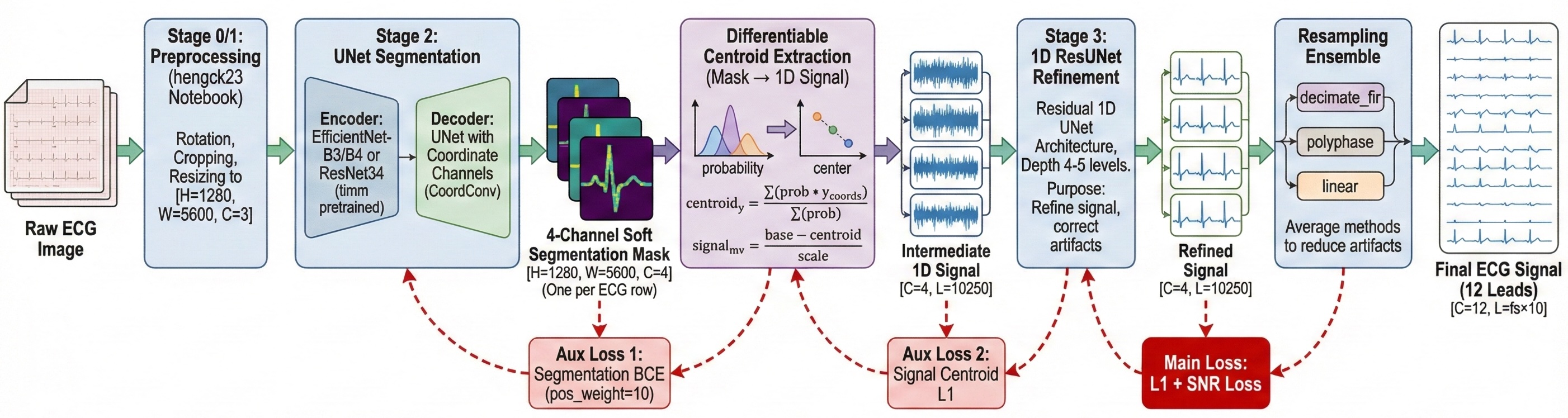
  "content": "<p>Thanks to the organizers for this interesting competition! Here's a summary of our approach.</p>\n<hr>\n<h2>Overview</h2>\n<p>Our solution is based on an <strong>End-to-End (E2E) deep learning pipeline</strong> that directly predicts ECG time-series signals from ECG images. The key insight was to combine image segmentation with signal refinement in a single differentiable pipeline.</p>\n<hr>\n<h2>Pipeline Architecture</h2>\n<p><img src=\"https://www.googleapis.com/download/storage/v1/b/kaggle-user-content/o/inbox%2F2848721%2F1314856109fa4672e8b6ded6a3a4a12a%2Fpipeline.jpg?generation=1769129908598386&amp;alt=media\" alt=\"\"></p>\n<pre><code>ECG Image (Stage 1 preprocessed)\n    │  [H=1280, W=5600, C=3]\n    ↓\nStage 2: UNet Segmentation (4-channel soft mask)\n    │  [H=1280, W=5600, C=4]\n    │  ← Aux Loss 1: Segmentation BCE Loss\n    ↓\nDifferentiable Centroid Extraction (mask → 1D signal)\n    │  [C=4, L=10250]\n    │  ← Aux Loss 2: Signal Centroid L1 Loss\n    ↓\nStage 3: 1D ResUNet Refinement\n    │  [C=4, L=10250]\n    │  ← Main Loss: L1 + SNR Loss\n    ↓\nResampling Ensemble (decimate_fir + polyphase + linear)\n    │  [C=4, L=fs×10] (e.g., 5000 for fs=500Hz)\n    ↓\nFinal ECG Signal (12 leads)\n</code></pre>\n<h3>Stage 0/Stage 1: Preprocessing (from hengck23's notebook)</h3>\n<ul>\n<li>We used <strong>hengck23's excellent public notebook</strong> for preprocessing</li>\n<li>Includes image rotation correction, cropping, and resizing to 5600×1280</li>\n</ul>\n<h3>Stage 2: UNet Segmentation</h3>\n<ul>\n<li><strong>Encoder</strong>: EfficientNet-B3/B4 or ResNet34 (timm pretrained)</li>\n<li><strong>Decoder</strong>: UNet with coordinate channels (CoordConv-style)</li>\n<li><strong>Output</strong>: 4-channel soft segmentation mask (one per ECG row)</li>\n<li><strong>Loss</strong>: BCE with pos_weight=10 for class imbalance</li>\n</ul>\n<h3>Differentiable Centroid Conversion</h3>\n<p>This was a key component that enabled end-to-end training:</p>\n<pre><code># For each column, compute weighted centroid of the probability distribution\ny_coords = torch.arange(H).view(1, 1, H, 1)\nprob_sum = seg_prob.sum(dim=2) + eps\ncentroid_y = (seg_prob * y_coords).sum(dim=2) / prob_sum\n\n# Convert pixel position to mV\nsignal_mv = (base_y_position - centroid_y) / y_scale\n</code></pre>\n<p>This allows gradients to flow from the signal loss back through the segmentation network.</p>\n<h3>Stage 3: 1D ResUNet</h3>\n<ul>\n<li><strong>Architecture</strong>: Residual 1D UNet</li>\n<li><strong>Input/Output</strong>: 4 channels (corresponding to 4 ECG rows)</li>\n<li><strong>Depth</strong>: 4-5 levels</li>\n<li><strong>Purpose</strong>: Refine the centroid-extracted signal, correct artifacts</li>\n</ul>\n<hr>\n<h2>Training Strategy</h2>\n<h3>Loss Function</h3>\n<p>Combined segmentation and signal losses with scheduled weighting:</p>\n<pre><code># Early training: focus on segmentation\n# Later training: shift focus to signal quality\nseg_weight = seg_start + (seg_end - seg_start) * progress\nsignal_weight = sig_start + (sig_end - sig_start) * progress\n\nloss = seg_weight * seg_bce_loss + signal_weight * (l1_loss + snr_loss)\n</code></pre>\n<h3>Key Training Details</h3>\n<ul>\n<li><strong>Optimizer</strong>: AdamW (lr=0.005, weight_decay=1e-4)</li>\n<li><strong>Scheduler</strong>: Cosine annealing (60 epochs schedule, 32 epochs training)</li>\n<li><strong>Batch size</strong>: 4 with gradient accumulation (effective batch 16)</li>\n<li><strong>Precision</strong>: FP32 (FP16 caused NaN issues)</li>\n<li><strong>EMA</strong>: Enabled (decay=0.995)</li>\n<li><strong>All-data training</strong>: No validation split for final models</li>\n</ul>\n<h3>Data Augmentation</h3>\n<p>Augmentation was crucial for generalization:</p>\n<table>\n<thead>\n<tr>\n<th>Augmentation</th>\n<th>Probability</th>\n<th>Impact</th>\n</tr>\n</thead>\n<tbody>\n<tr>\n<td><strong>Horizontal Flip</strong></td>\n<td>0.5</td>\n<td><strong>+0.6 dB</strong> (biggest improvement!)</td>\n</tr>\n<tr>\n<td>Grayscale</td>\n<td>0.2</td>\n<td>Helps with color variation</td>\n</tr>\n<tr>\n<td>Brightness/Contrast</td>\n<td>0.3</td>\n<td>Robustness to lighting</td>\n</tr>\n<tr>\n<td>JPEG Compression</td>\n<td>0.2</td>\n<td>Handles low-quality scans</td>\n</tr>\n<tr>\n<td>Cutout</td>\n<td>0.2</td>\n<td>Handles occlusions/damage</td>\n</tr>\n<tr>\n<td>Gaussian Noise</td>\n<td>0.2</td>\n<td>Handles sensor noise</td>\n</tr>\n</tbody>\n</table>\n<p>The horizontal flip augmentation was surprisingly effective (+0.6 dB), likely because it doubled the effective training data and helped the model learn orientation-invariant features.</p>\n<hr>\n<h2>Ensemble Strategy</h2>\n<h3>Model Diversity</h3>\n<p>We trained multiple models with different configurations:</p>\n<table>\n<thead>\n<tr>\n<th>Model</th>\n<th>Encoder</th>\n<th>Stage3</th>\n<th>hflip</th>\n<th>LB Score(w/o Resampling Ensemble)</th>\n</tr>\n</thead>\n<tbody>\n<tr>\n<td>m009</td>\n<td>ResNet34</td>\n<td>resunet1d (d=4)</td>\n<td>0.0</td>\n<td>20.02</td>\n</tr>\n<tr>\n<td>m010</td>\n<td>EfficientNet-B3</td>\n<td>resunet1d (d=4)</td>\n<td>0.0</td>\n<td>20.21</td>\n</tr>\n<tr>\n<td>m013</td>\n<td>ResNet34</td>\n<td>resunet1d (d=4)</td>\n<td>0.5</td>\n<td>20.64</td>\n</tr>\n<tr>\n<td>m014</td>\n<td>EfficientNet-B3</td>\n<td>resunet1d (d=4)</td>\n<td>0.5</td>\n<td>20.84</td>\n</tr>\n<tr>\n<td>m018</td>\n<td>EfficientNet-B3</td>\n<td>resunet1d (d=5)</td>\n<td>0.5</td>\n<td>20.87</td>\n</tr>\n<tr>\n<td>m020</td>\n<td>EfficientNet-B4</td>\n<td>resunet1d (d=4)</td>\n<td>0.5</td>\n<td>20.61</td>\n</tr>\n</tbody>\n</table>\n<h3>Final Ensemble</h3>\n<pre><code>models = ['m009', 'm010', 'm013', 'm014', 'm018', 'm020']\nweights = [0.05, 0.1, 0.2, 0.25, 0.25, 0.15]\n</code></pre>\n<p>Weighted average based on single-model performance, with slight diversity bonus for different architectures.</p>\n<h3>Resampling Ensemble</h3>\n<p>A subtle but effective technique: <strong>ensemble multiple resampling methods</strong> when converting from model output length to target sampling frequency.</p>\n<pre><code>ensemble_methods = ['decimate_fir', 'polyphase', 'linear']\n</code></pre>\n<p>Different resampling algorithms introduce different artifacts (especially at signal edges). Averaging them cancels out method-specific artifacts.</p>\n<hr>\n<h2>What Worked</h2>\n<ol>\n<li><strong>End-to-end training</strong> - Joint optimization of segmentation and signal extraction was better than separate stages</li>\n<li><strong>Horizontal flip augmentation</strong> - Surprisingly gave +0.6 dB improvement</li>\n<li><strong>EfficientNet encoders</strong> - Consistently +0.2 dB over ResNet</li>\n<li><strong>Deeper Stage3</strong> - depth=5 helped capture longer-range dependencies</li>\n<li><strong>Resampling ensemble</strong> - Reduced edge artifacts</li>\n<li><strong>Model diversity in ensemble</strong> - Mixing architectures and augmentation settings</li>\n</ol>\n<hr>\n<h2>What Didn't Work</h2>\n<ol>\n<li><strong>BiLSTM for Stage3</strong> - Worse than ResUNet (-0.9 dB)</li>\n<li><strong>Higher resolution (7200×1280)</strong> - No improvement, slower training</li>\n<li><strong>Larger output_length (15000)</strong> - Marginal improvement not worth complexity</li>\n<li><strong>ConvNeXt encoder</strong> - Training instability issues</li>\n</ol>\n<hr>\n<h2>Acknowledgments</h2>\n<p><strong>Huge thanks to <a href=\"https://www.kaggle.com/hengck23\" target=\"_blank\">@hengck23</a></strong> for the excellent public notebooks! Our Stage 1 preprocessing is entirely based on hengck23's work, which provided the foundation for our pipeline. The clean, standardized images from Stage 1 were essential for training our E2E model effectively.</p>\n<p>Thanks also to the Kaggle community for the insightful discussions throughout the competition</p>",
  "messages": [
    {
      "id": "3395432",
      "postDate": "01/23/2026 00:59:29",
      "content": "<p>Thanks to the organizers for this interesting competition! Here's a summary of our approach.</p>\n<hr>\n<h2>Overview</h2>\n<p>Our solution is based on an <strong>End-to-End (E2E) deep learning pipeline</strong> that directly predicts ECG time-series signals from ECG images. The key insight was to combine image segmentation with signal refinement in a single differentiable pipeline.</p>\n<hr>\n<h2>Pipeline Architecture</h2>\n<p><img src=\"https://www.googleapis.com/download/storage/v1/b/kaggle-user-content/o/inbox%2F2848721%2F1314856109fa4672e8b6ded6a3a4a12a%2Fpipeline.jpg?generation=1769129908598386&amp;alt=media\" alt=\"\"></p>\n<pre><code>ECG Image (Stage 1 preprocessed)\n    │  [H=1280, W=5600, C=3]\n    ↓\nStage 2: UNet Segmentation (4-channel soft mask)\n    │  [H=1280, W=5600, C=4]\n    │  ← Aux Loss 1: Segmentation BCE Loss\n    ↓\nDifferentiable Centroid Extraction (mask → 1D signal)\n    │  [C=4, L=10250]\n    │  ← Aux Loss 2: Signal Centroid L1 Loss\n    ↓\nStage 3: 1D ResUNet Refinement\n    │  [C=4, L=10250]\n    │  ← Main Loss: L1 + SNR Loss\n    ↓\nResampling Ensemble (decimate_fir + polyphase + linear)\n    │  [C=4, L=fs×10] (e.g., 5000 for fs=500Hz)\n    ↓\nFinal ECG Signal (12 leads)\n</code></pre>\n<h3>Stage 0/Stage 1: Preprocessing (from hengck23's notebook)</h3>\n<ul>\n<li>We used <strong>hengck23's excellent public notebook</strong> for preprocessing</li>\n<li>Includes image rotation correction, cropping, and resizing to 5600×1280</li>\n</ul>\n<h3>Stage 2: UNet Segmentation</h3>\n<ul>\n<li><strong>Encoder</strong>: EfficientNet-B3/B4 or ResNet34 (timm pretrained)</li>\n<li><strong>Decoder</strong>: UNet with coordinate channels (CoordConv-style)</li>\n<li><strong>Output</strong>: 4-channel soft segmentation mask (one per ECG row)</li>\n<li><strong>Loss</strong>: BCE with pos_weight=10 for class imbalance</li>\n</ul>\n<h3>Differentiable Centroid Conversion</h3>\n<p>This was a key component that enabled end-to-end training:</p>\n<pre><code># For each column, compute weighted centroid of the probability distribution\ny_coords = torch.arange(H).view(1, 1, H, 1)\nprob_sum = seg_prob.sum(dim=2) + eps\ncentroid_y = (seg_prob * y_coords).sum(dim=2) / prob_sum\n\n# Convert pixel position to mV\nsignal_mv = (base_y_position - centroid_y) / y_scale\n</code></pre>\n<p>This allows gradients to flow from the signal loss back through the segmentation network.</p>\n<h3>Stage 3: 1D ResUNet</h3>\n<ul>\n<li><strong>Architecture</strong>: Residual 1D UNet</li>\n<li><strong>Input/Output</strong>: 4 channels (corresponding to 4 ECG rows)</li>\n<li><strong>Depth</strong>: 4-5 levels</li>\n<li><strong>Purpose</strong>: Refine the centroid-extracted signal, correct artifacts</li>\n</ul>\n<hr>\n<h2>Training Strategy</h2>\n<h3>Loss Function</h3>\n<p>Combined segmentation and signal losses with scheduled weighting:</p>\n<pre><code># Early training: focus on segmentation\n# Later training: shift focus to signal quality\nseg_weight = seg_start + (seg_end - seg_start) * progress\nsignal_weight = sig_start + (sig_end - sig_start) * progress\n\nloss = seg_weight * seg_bce_loss + signal_weight * (l1_loss + snr_loss)\n</code></pre>\n<h3>Key Training Details</h3>\n<ul>\n<li><strong>Optimizer</strong>: AdamW (lr=0.005, weight_decay=1e-4)</li>\n<li><strong>Scheduler</strong>: Cosine annealing (60 epochs schedule, 32 epochs training)</li>\n<li><strong>Batch size</strong>: 4 with gradient accumulation (effective batch 16)</li>\n<li><strong>Precision</strong>: FP32 (FP16 caused NaN issues)</li>\n<li><strong>EMA</strong>: Enabled (decay=0.995)</li>\n<li><strong>All-data training</strong>: No validation split for final models</li>\n</ul>\n<h3>Data Augmentation</h3>\n<p>Augmentation was crucial for generalization:</p>\n<table>\n<thead>\n<tr>\n<th>Augmentation</th>\n<th>Probability</th>\n<th>Impact</th>\n</tr>\n</thead>\n<tbody>\n<tr>\n<td><strong>Horizontal Flip</strong></td>\n<td>0.5</td>\n<td><strong>+0.6 dB</strong> (biggest improvement!)</td>\n</tr>\n<tr>\n<td>Grayscale</td>\n<td>0.2</td>\n<td>Helps with color variation</td>\n</tr>\n<tr>\n<td>Brightness/Contrast</td>\n<td>0.3</td>\n<td>Robustness to lighting</td>\n</tr>\n<tr>\n<td>JPEG Compression</td>\n<td>0.2</td>\n<td>Handles low-quality scans</td>\n</tr>\n<tr>\n<td>Cutout</td>\n<td>0.2</td>\n<td>Handles occlusions/damage</td>\n</tr>\n<tr>\n<td>Gaussian Noise</td>\n<td>0.2</td>\n<td>Handles sensor noise</td>\n</tr>\n</tbody>\n</table>\n<p>The horizontal flip augmentation was surprisingly effective (+0.6 dB), likely because it doubled the effective training data and helped the model learn orientation-invariant features.</p>\n<hr>\n<h2>Ensemble Strategy</h2>\n<h3>Model Diversity</h3>\n<p>We trained multiple models with different configurations:</p>\n<table>\n<thead>\n<tr>\n<th>Model</th>\n<th>Encoder</th>\n<th>Stage3</th>\n<th>hflip</th>\n<th>LB Score(w/o Resampling Ensemble)</th>\n</tr>\n</thead>\n<tbody>\n<tr>\n<td>m009</td>\n<td>ResNet34</td>\n<td>resunet1d (d=4)</td>\n<td>0.0</td>\n<td>20.02</td>\n</tr>\n<tr>\n<td>m010</td>\n<td>EfficientNet-B3</td>\n<td>resunet1d (d=4)</td>\n<td>0.0</td>\n<td>20.21</td>\n</tr>\n<tr>\n<td>m013</td>\n<td>ResNet34</td>\n<td>resunet1d (d=4)</td>\n<td>0.5</td>\n<td>20.64</td>\n</tr>\n<tr>\n<td>m014</td>\n<td>EfficientNet-B3</td>\n<td>resunet1d (d=4)</td>\n<td>0.5</td>\n<td>20.84</td>\n</tr>\n<tr>\n<td>m018</td>\n<td>EfficientNet-B3</td>\n<td>resunet1d (d=5)</td>\n<td>0.5</td>\n<td>20.87</td>\n</tr>\n<tr>\n<td>m020</td>\n<td>EfficientNet-B4</td>\n<td>resunet1d (d=4)</td>\n<td>0.5</td>\n<td>20.61</td>\n</tr>\n</tbody>\n</table>\n<h3>Final Ensemble</h3>\n<pre><code>models = ['m009', 'm010', 'm013', 'm014', 'm018', 'm020']\nweights = [0.05, 0.1, 0.2, 0.25, 0.25, 0.15]\n</code></pre>\n<p>Weighted average based on single-model performance, with slight diversity bonus for different architectures.</p>\n<h3>Resampling Ensemble</h3>\n<p>A subtle but effective technique: <strong>ensemble multiple resampling methods</strong> when converting from model output length to target sampling frequency.</p>\n<pre><code>ensemble_methods = ['decimate_fir', 'polyphase', 'linear']\n</code></pre>\n<p>Different resampling algorithms introduce different artifacts (especially at signal edges). Averaging them cancels out method-specific artifacts.</p>\n<hr>\n<h2>What Worked</h2>\n<ol>\n<li><strong>End-to-end training</strong> - Joint optimization of segmentation and signal extraction was better than separate stages</li>\n<li><strong>Horizontal flip augmentation</strong> - Surprisingly gave +0.6 dB improvement</li>\n<li><strong>EfficientNet encoders</strong> - Consistently +0.2 dB over ResNet</li>\n<li><strong>Deeper Stage3</strong> - depth=5 helped capture longer-range dependencies</li>\n<li><strong>Resampling ensemble</strong> - Reduced edge artifacts</li>\n<li><strong>Model diversity in ensemble</strong> - Mixing architectures and augmentation settings</li>\n</ol>\n<hr>\n<h2>What Didn't Work</h2>\n<ol>\n<li><strong>BiLSTM for Stage3</strong> - Worse than ResUNet (-0.9 dB)</li>\n<li><strong>Higher resolution (7200×1280)</strong> - No improvement, slower training</li>\n<li><strong>Larger output_length (15000)</strong> - Marginal improvement not worth complexity</li>\n<li><strong>ConvNeXt encoder</strong> - Training instability issues</li>\n</ol>\n<hr>\n<h2>Acknowledgments</h2>\n<p><strong>Huge thanks to <a href=\"https://www.kaggle.com/hengck23\" target=\"_blank\">@hengck23</a></strong> for the excellent public notebooks! Our Stage 1 preprocessing is entirely based on hengck23's work, which provided the foundation for our pipeline. The clean, standardized images from Stage 1 were essential for training our E2E model effectively.</p>\n<p>Thanks also to the Kaggle community for the insightful discussions throughout the competition</p>",
      "rawMarkdown": "Thanks to the organizers for this interesting competition! Here's a summary of our approach.\n\n---\n\n## Overview\n\nOur solution is based on an **End-to-End (E2E) deep learning pipeline** that directly predicts ECG time-series signals from ECG images. The key insight was to combine image segmentation with signal refinement in a single differentiable pipeline.\n\n---\n\n## Pipeline Architecture\n\n![](https://www.googleapis.com/download/storage/v1/b/kaggle-user-content/o/inbox%2F2848721%2F1314856109fa4672e8b6ded6a3a4a12a%2Fpipeline.jpg?generation=1769129908598386&alt=media)\n\n```\nECG Image (Stage 1 preprocessed)\n    │  [H=1280, W=5600, C=3]\n    ↓\nStage 2: UNet Segmentation (4-channel soft mask)\n    │  [H=1280, W=5600, C=4]\n    │  ← Aux Loss 1: Segmentation BCE Loss\n    ↓\nDifferentiable Centroid Extraction (mask → 1D signal)\n    │  [C=4, L=10250]\n    │  ← Aux Loss 2: Signal Centroid L1 Loss\n    ↓\nStage 3: 1D ResUNet Refinement\n    │  [C=4, L=10250]\n    │  ← Main Loss: L1 + SNR Loss\n    ↓\nResampling Ensemble (decimate_fir + polyphase + linear)\n    │  [C=4, L=fs×10] (e.g., 5000 for fs=500Hz)\n    ↓\nFinal ECG Signal (12 leads)\n```\n\n\n### Stage 0/Stage 1: Preprocessing (from hengck23's notebook)\n- We used **hengck23's excellent public notebook** for preprocessing\n- Includes image rotation correction, cropping, and resizing to 5600×1280\n\n### Stage 2: UNet Segmentation\n- **Encoder**: EfficientNet-B3/B4 or ResNet34 (timm pretrained)\n- **Decoder**: UNet with coordinate channels (CoordConv-style)\n- **Output**: 4-channel soft segmentation mask (one per ECG row)\n- **Loss**: BCE with pos_weight=10 for class imbalance\n\n### Differentiable Centroid Conversion\nThis was a key component that enabled end-to-end training:\n\n```python\n# For each column, compute weighted centroid of the probability distribution\ny_coords = torch.arange(H).view(1, 1, H, 1)\nprob_sum = seg_prob.sum(dim=2) + eps\ncentroid_y = (seg_prob * y_coords).sum(dim=2) / prob_sum\n\n# Convert pixel position to mV\nsignal_mv = (base_y_position - centroid_y) / y_scale\n```\n\nThis allows gradients to flow from the signal loss back through the segmentation network.\n\n### Stage 3: 1D ResUNet\n- **Architecture**: Residual 1D UNet\n- **Input/Output**: 4 channels (corresponding to 4 ECG rows)\n- **Depth**: 4-5 levels\n- **Purpose**: Refine the centroid-extracted signal, correct artifacts\n\n---\n\n## Training Strategy\n\n### Loss Function\nCombined segmentation and signal losses with scheduled weighting:\n\n```python\n# Early training: focus on segmentation\n# Later training: shift focus to signal quality\nseg_weight = seg_start + (seg_end - seg_start) * progress\nsignal_weight = sig_start + (sig_end - sig_start) * progress\n\nloss = seg_weight * seg_bce_loss + signal_weight * (l1_loss + snr_loss)\n```\n\n### Key Training Details\n- **Optimizer**: AdamW (lr=0.005, weight_decay=1e-4)\n- **Scheduler**: Cosine annealing (60 epochs schedule, 32 epochs training)\n- **Batch size**: 4 with gradient accumulation (effective batch 16)\n- **Precision**: FP32 (FP16 caused NaN issues)\n- **EMA**: Enabled (decay=0.995)\n- **All-data training**: No validation split for final models\n\n### Data Augmentation\nAugmentation was crucial for generalization:\n\n| Augmentation | Probability | Impact |\n|--------------|-------------|--------|\n| **Horizontal Flip** | 0.5 | **+0.6 dB** (biggest improvement!) |\n| Grayscale | 0.2 | Helps with color variation |\n| Brightness/Contrast | 0.3 | Robustness to lighting |\n| JPEG Compression | 0.2 | Handles low-quality scans |\n| Cutout | 0.2 | Handles occlusions/damage |\n| Gaussian Noise | 0.2 | Handles sensor noise |\n\nThe horizontal flip augmentation was surprisingly effective (+0.6 dB), likely because it doubled the effective training data and helped the model learn orientation-invariant features.\n\n---\n\n## Ensemble Strategy\n\n### Model Diversity\nWe trained multiple models with different configurations:\n\n| Model | Encoder | Stage3 | hflip | LB Score(w/o Resampling Ensemble) |\n|-------|---------|--------|-------|----------|\n| m009 | ResNet34 | resunet1d (d=4) | 0.0 | 20.02 |\n| m010 | EfficientNet-B3 | resunet1d (d=4) | 0.0 | 20.21 |\n| m013 | ResNet34 | resunet1d (d=4) | 0.5 | 20.64 |\n| m014 | EfficientNet-B3 | resunet1d (d=4) | 0.5 | 20.84 |\n| m018 | EfficientNet-B3 | resunet1d (d=5) | 0.5 | 20.87 |\n| m020 | EfficientNet-B4 | resunet1d (d=4) | 0.5 | 20.61 |\n\n### Final Ensemble\n```python\nmodels = ['m009', 'm010', 'm013', 'm014', 'm018', 'm020']\nweights = [0.05, 0.1, 0.2, 0.25, 0.25, 0.15]\n```\n\nWeighted average based on single-model performance, with slight diversity bonus for different architectures.\n\n### Resampling Ensemble\nA subtle but effective technique: **ensemble multiple resampling methods** when converting from model output length to target sampling frequency.\n\n```python\nensemble_methods = ['decimate_fir', 'polyphase', 'linear']\n```\n\nDifferent resampling algorithms introduce different artifacts (especially at signal edges). Averaging them cancels out method-specific artifacts.\n\n---\n\n## What Worked\n\n1. **End-to-end training** - Joint optimization of segmentation and signal extraction was better than separate stages\n2. **Horizontal flip augmentation** - Surprisingly gave +0.6 dB improvement\n3. **EfficientNet encoders** - Consistently +0.2 dB over ResNet\n4. **Deeper Stage3** - depth=5 helped capture longer-range dependencies\n5. **Resampling ensemble** - Reduced edge artifacts\n6. **Model diversity in ensemble** - Mixing architectures and augmentation settings\n\n---\n\n## What Didn't Work\n\n1. **BiLSTM for Stage3** - Worse than ResUNet (-0.9 dB)\n2. **Higher resolution (7200×1280)** - No improvement, slower training\n3. **Larger output_length (15000)** - Marginal improvement not worth complexity\n4. **ConvNeXt encoder** - Training instability issues\n\n\n---\n\n## Acknowledgments\n\n**Huge thanks to [@hengck23](https://www.kaggle.com/hengck23)** for the excellent public notebooks! Our Stage 1 preprocessing is entirely based on hengck23's work, which provided the foundation for our pipeline. The clean, standardized images from Stage 1 were essential for training our E2E model effectively.\n\nThanks also to the Kaggle community for the insightful discussions throughout the competition",
      "votes": null
    },
    {
      "id": "3395551",
      "postDate": "01/23/2026 07:32:16",
      "content": "<p>Great work! Thank you for sharing. What is the ground-truth (GT) mask used for the segmentation part?</p>",
      "rawMarkdown": "Great work! Thank you for sharing. What is the ground-truth (GT) mask used for the segmentation part?",
      "votes": null
    },
    {
      "id": "3395675",
      "postDate": "01/23/2026 12:54:44",
      "content": "<p>Thank you for the comment!</p>\n<p>The GT mask is generated using the <code>render_signal</code> function provided below. The parameters for <code>render_signal</code> were optimized using the following procedure:</p>\n<ol>\n<li>Crop the top part (H=1280) of the 0001 output from Stage 1 and remove the grid using <code>remove_grid_extract_ecg</code>.</li>\n<li>Render the Ground Truth (GT) using render_signal to match the size from Step 1, and search for the parameters that maximize the Dice coefficient against the image from Step 1.</li>\n</ol>\n<p>The attached image shows the result after optimization. Since it depends on the accuracy of Stage 1, it is not a strictly precise segmentation mask, but it was sufficient for the loss calculation during the early stages of training.</p>\n<p><img src=\"https://www.googleapis.com/download/storage/v1/b/kaggle-forum-message-attachments/o/inbox%2F2848721%2F4228efafd122f3c0d729a6714c7ba76d%2F2026-01-23%2021.20.19.png?generation=1769170847408910&amp;alt=media\" alt=\"\"></p>\n<pre><code>def remove_grid_extract_ecg(img, sat_thresh=50, val_thresh=150):\n    \"\"\"\n    Remove colored grid and extract black ECG lines.\n\n    Args:\n        img: BGR image\n        sat_thresh: Saturation threshold (pixels below this are considered non-colored)\n        val_thresh: Value threshold (pixels below this are considered dark)\n\n    Returns:\n        Binary mask of ECG lines, result image with grid removed\n    \"\"\"\n    hsv = cv2.cvtColor(img, cv2.COLOR_BGR2HSV)\n    saturation = hsv[:, :, 1]\n    value = hsv[:, :, 2]\n\n    # Black ECG lines: low saturation AND low value\n    ecg_mask = (saturation &lt; sat_thresh) &amp; (value &lt; val_thresh)\n\n    # Clean up\n    kernel = np.ones((2, 2), np.uint8)\n    ecg_mask_clean = cv2.morphologyEx(\n        ecg_mask.astype(np.uint8) * 255, cv2.MORPH_CLOSE, kernel\n    )\n\n    # Create result image\n    result = np.ones_like(img) * 255\n    result[ecg_mask_clean &gt; 0] = [0, 0, 0]\n\n    return ecg_mask_clean, result\n\ndef render_signal(gt, y_positions, y_scale, sigma=3.0):\n    \"\"\"\n    Render GT signal with 1px per point.\n\n    Args:\n        gt: 4-channel GT signal (4, signal_len)\n        y_positions: Y-coordinates for each row (based on ORIGINAL_SIZE)\n        y_scale: Scale in Y direction\n        sigma: Standard deviation for Gaussian blur\n\n    Returns:\n        Rendered image (h, signal_len)\n    \"\"\"\n    n_rows, signal_len = gt.shape\n    h = ORIGINAL_SIZE[1]\n    img = np.zeros((h, signal_len), dtype=np.uint8)\n\n    current_y_positions = [y for y in y_positions]\n\n    for row_idx in range(n_rows):\n        signal = gt[row_idx]\n\n        # Skip if signal is all zeros (or very small)\n        if np.abs(signal).max() &lt; 1e-6:\n            continue\n\n        y_center = current_y_positions[row_idx]\n\n        # Signal scaling (signal=0 corresponds to y_center)\n        signal_norm = signal * y_scale\n        y_coords = y_center - signal_norm\n        y_coords = np.clip(y_coords, 0, h - 1).astype(np.int32)\n\n        # Draw 1px per point\n        img[y_coords, np.arange(signal_len)] = 255\n\n    # --- Step 2: \"Thicken\" lines using Gaussian Blur ---\n    if sigma &gt; 0:\n        # Kernel size is typically about 6 times sigma (must be odd)\n        k_size = int(6 * sigma) | 1  # Hack to ensure odd number\n\n        # Blur in both X and Y directions with (k_size, k_size)\n        # *Note: Change to (1, k_size) if you want to preserve sharpness in the X direction (time axis).\n        img = cv2.GaussianBlur(img, (1, k_size), sigma)\n\n        # --- Step 3: Intensity Normalization ---\n        # Since blurring reduces peak values below 255, restore max value to 255.\n        # Without this, the balance of the Dice coefficient (numerator/denominator) might be skewed.\n        max_val = img.max()\n        if max_val &gt; 0:\n            img = (img.astype(np.float32) / max_val * 255).astype(np.uint8)\n\n    return img\n</code></pre>",
      "rawMarkdown": "Thank you for the comment!\n\nThe GT mask is generated using the `render_signal` function provided below. The parameters for `render_signal` were optimized using the following procedure:\n\n1. Crop the top part (H=1280) of the 0001 output from Stage 1 and remove the grid using `remove_grid_extract_ecg`.\n1. Render the Ground Truth (GT) using render_signal to match the size from Step 1, and search for the parameters that maximize the Dice coefficient against the image from Step 1.\n\nThe attached image shows the result after optimization. Since it depends on the accuracy of Stage 1, it is not a strictly precise segmentation mask, but it was sufficient for the loss calculation during the early stages of training.\n\n![](https://www.googleapis.com/download/storage/v1/b/kaggle-forum-message-attachments/o/inbox%2F2848721%2F4228efafd122f3c0d729a6714c7ba76d%2F2026-01-23%2021.20.19.png?generation=1769170847408910&alt=media)\n\n```python\ndef remove_grid_extract_ecg(img, sat_thresh=50, val_thresh=150):\n    \"\"\"\n    Remove colored grid and extract black ECG lines.\n\n    Args:\n        img: BGR image\n        sat_thresh: Saturation threshold (pixels below this are considered non-colored)\n        val_thresh: Value threshold (pixels below this are considered dark)\n\n    Returns:\n        Binary mask of ECG lines, result image with grid removed\n    \"\"\"\n    hsv = cv2.cvtColor(img, cv2.COLOR_BGR2HSV)\n    saturation = hsv[:, :, 1]\n    value = hsv[:, :, 2]\n\n    # Black ECG lines: low saturation AND low value\n    ecg_mask = (saturation < sat_thresh) & (value < val_thresh)\n\n    # Clean up\n    kernel = np.ones((2, 2), np.uint8)\n    ecg_mask_clean = cv2.morphologyEx(\n        ecg_mask.astype(np.uint8) * 255, cv2.MORPH_CLOSE, kernel\n    )\n\n    # Create result image\n    result = np.ones_like(img) * 255\n    result[ecg_mask_clean > 0] = [0, 0, 0]\n\n    return ecg_mask_clean, result\n\ndef render_signal(gt, y_positions, y_scale, sigma=3.0):\n    \"\"\"\n    Render GT signal with 1px per point.\n\n    Args:\n        gt: 4-channel GT signal (4, signal_len)\n        y_positions: Y-coordinates for each row (based on ORIGINAL_SIZE)\n        y_scale: Scale in Y direction\n        sigma: Standard deviation for Gaussian blur\n\n    Returns:\n        Rendered image (h, signal_len)\n    \"\"\"\n    n_rows, signal_len = gt.shape\n    h = ORIGINAL_SIZE[1]\n    img = np.zeros((h, signal_len), dtype=np.uint8)\n\n    current_y_positions = [y for y in y_positions]\n\n    for row_idx in range(n_rows):\n        signal = gt[row_idx]\n\n        # Skip if signal is all zeros (or very small)\n        if np.abs(signal).max() < 1e-6:\n            continue\n\n        y_center = current_y_positions[row_idx]\n\n        # Signal scaling (signal=0 corresponds to y_center)\n        signal_norm = signal * y_scale\n        y_coords = y_center - signal_norm\n        y_coords = np.clip(y_coords, 0, h - 1).astype(np.int32)\n\n        # Draw 1px per point\n        img[y_coords, np.arange(signal_len)] = 255\n\n    # --- Step 2: \"Thicken\" lines using Gaussian Blur ---\n    if sigma > 0:\n        # Kernel size is typically about 6 times sigma (must be odd)\n        k_size = int(6 * sigma) | 1  # Hack to ensure odd number\n\n        # Blur in both X and Y directions with (k_size, k_size)\n        # *Note: Change to (1, k_size) if you want to preserve sharpness in the X direction (time axis).\n        img = cv2.GaussianBlur(img, (1, k_size), sigma)\n\n        # --- Step 3: Intensity Normalization ---\n        # Since blurring reduces peak values below 255, restore max value to 255.\n        # Without this, the balance of the Dice coefficient (numerator/denominator) might be skewed.\n        max_val = img.max()\n        if max_val > 0:\n            img = (img.astype(np.float32) / max_val * 255).astype(np.uint8)\n\n    return img\n```",
      "votes": null
    }
  ],
  "comments": [
    {
      "id": 3395551,
      "author_name": "vandongtran",
      "author_url": "",
      "post_date": "01/23/2026 07:32:16",
      "content": "<p>Great work! Thank you for sharing. What is the ground-truth (GT) mask used for the segmentation part?</p>",
      "votes": null,
      "replies": [
        {
          "id": 3395675,
          "author_name": "maruichi01",
          "author_url": "",
          "post_date": "01/23/2026 12:54:44",
          "content": "<p>Thank you for the comment!</p>\n<p>The GT mask is generated using the <code>render_signal</code> function provided below. The parameters for <code>render_signal</code> were optimized using the following procedure:</p>\n<ol>\n<li>Crop the top part (H=1280) of the 0001 output from Stage 1 and remove the grid using <code>remove_grid_extract_ecg</code>.</li>\n<li>Render the Ground Truth (GT) using render_signal to match the size from Step 1, and search for the parameters that maximize the Dice coefficient against the image from Step 1.</li>\n</ol>\n<p>The attached image shows the result after optimization. Since it depends on the accuracy of Stage 1, it is not a strictly precise segmentation mask, but it was sufficient for the loss calculation during the early stages of training.</p>\n<p><img src=\"https://www.googleapis.com/download/storage/v1/b/kaggle-forum-message-attachments/o/inbox%2F2848721%2F4228efafd122f3c0d729a6714c7ba76d%2F2026-01-23%2021.20.19.png?generation=1769170847408910&amp;alt=media\" alt=\"\"></p>\n<pre><code>def remove_grid_extract_ecg(img, sat_thresh=50, val_thresh=150):\n    \"\"\"\n    Remove colored grid and extract black ECG lines.\n\n    Args:\n        img: BGR image\n        sat_thresh: Saturation threshold (pixels below this are considered non-colored)\n        val_thresh: Value threshold (pixels below this are considered dark)\n\n    Returns:\n        Binary mask of ECG lines, result image with grid removed\n    \"\"\"\n    hsv = cv2.cvtColor(img, cv2.COLOR_BGR2HSV)\n    saturation = hsv[:, :, 1]\n    value = hsv[:, :, 2]\n\n    # Black ECG lines: low saturation AND low value\n    ecg_mask = (saturation &lt; sat_thresh) &amp; (value &lt; val_thresh)\n\n    # Clean up\n    kernel = np.ones((2, 2), np.uint8)\n    ecg_mask_clean = cv2.morphologyEx(\n        ecg_mask.astype(np.uint8) * 255, cv2.MORPH_CLOSE, kernel\n    )\n\n    # Create result image\n    result = np.ones_like(img) * 255\n    result[ecg_mask_clean &gt; 0] = [0, 0, 0]\n\n    return ecg_mask_clean, result\n\ndef render_signal(gt, y_positions, y_scale, sigma=3.0):\n    \"\"\"\n    Render GT signal with 1px per point.\n\n    Args:\n        gt: 4-channel GT signal (4, signal_len)\n        y_positions: Y-coordinates for each row (based on ORIGINAL_SIZE)\n        y_scale: Scale in Y direction\n        sigma: Standard deviation for Gaussian blur\n\n    Returns:\n        Rendered image (h, signal_len)\n    \"\"\"\n    n_rows, signal_len = gt.shape\n    h = ORIGINAL_SIZE[1]\n    img = np.zeros((h, signal_len), dtype=np.uint8)\n\n    current_y_positions = [y for y in y_positions]\n\n    for row_idx in range(n_rows):\n        signal = gt[row_idx]\n\n        # Skip if signal is all zeros (or very small)\n        if np.abs(signal).max() &lt; 1e-6:\n            continue\n\n        y_center = current_y_positions[row_idx]\n\n        # Signal scaling (signal=0 corresponds to y_center)\n        signal_norm = signal * y_scale\n        y_coords = y_center - signal_norm\n        y_coords = np.clip(y_coords, 0, h - 1).astype(np.int32)\n\n        # Draw 1px per point\n        img[y_coords, np.arange(signal_len)] = 255\n\n    # --- Step 2: \"Thicken\" lines using Gaussian Blur ---\n    if sigma &gt; 0:\n        # Kernel size is typically about 6 times sigma (must be odd)\n        k_size = int(6 * sigma) | 1  # Hack to ensure odd number\n\n        # Blur in both X and Y directions with (k_size, k_size)\n        # *Note: Change to (1, k_size) if you want to preserve sharpness in the X direction (time axis).\n        img = cv2.GaussianBlur(img, (1, k_size), sigma)\n\n        # --- Step 3: Intensity Normalization ---\n        # Since blurring reduces peak values below 255, restore max value to 255.\n        # Without this, the balance of the Dice coefficient (numerator/denominator) might be skewed.\n        max_val = img.max()\n        if max_val &gt; 0:\n            img = (img.astype(np.float32) / max_val * 255).astype(np.uint8)\n\n    return img\n</code></pre>",
          "votes": null,
          "replies": []
        }
      ]
    }
  ],
  "raw_markdown_by_id": {
    "3395432": "Thanks to the organizers for this interesting competition! Here's a summary of our approach.\n\n---\n\n## Overview\n\nOur solution is based on an **End-to-End (E2E) deep learning pipeline** that directly predicts ECG time-series signals from ECG images. The key insight was to combine image segmentation with signal refinement in a single differentiable pipeline.\n\n---\n\n## Pipeline Architecture\n\n![](https://www.googleapis.com/download/storage/v1/b/kaggle-user-content/o/inbox%2F2848721%2F1314856109fa4672e8b6ded6a3a4a12a%2Fpipeline.jpg?generation=1769129908598386&alt=media)\n\n```\nECG Image (Stage 1 preprocessed)\n    │  [H=1280, W=5600, C=3]\n    ↓\nStage 2: UNet Segmentation (4-channel soft mask)\n    │  [H=1280, W=5600, C=4]\n    │  ← Aux Loss 1: Segmentation BCE Loss\n    ↓\nDifferentiable Centroid Extraction (mask → 1D signal)\n    │  [C=4, L=10250]\n    │  ← Aux Loss 2: Signal Centroid L1 Loss\n    ↓\nStage 3: 1D ResUNet Refinement\n    │  [C=4, L=10250]\n    │  ← Main Loss: L1 + SNR Loss\n    ↓\nResampling Ensemble (decimate_fir + polyphase + linear)\n    │  [C=4, L=fs×10] (e.g., 5000 for fs=500Hz)\n    ↓\nFinal ECG Signal (12 leads)\n```\n\n\n### Stage 0/Stage 1: Preprocessing (from hengck23's notebook)\n- We used **hengck23's excellent public notebook** for preprocessing\n- Includes image rotation correction, cropping, and resizing to 5600×1280\n\n### Stage 2: UNet Segmentation\n- **Encoder**: EfficientNet-B3/B4 or ResNet34 (timm pretrained)\n- **Decoder**: UNet with coordinate channels (CoordConv-style)\n- **Output**: 4-channel soft segmentation mask (one per ECG row)\n- **Loss**: BCE with pos_weight=10 for class imbalance\n\n### Differentiable Centroid Conversion\nThis was a key component that enabled end-to-end training:\n\n```python\n# For each column, compute weighted centroid of the probability distribution\ny_coords = torch.arange(H).view(1, 1, H, 1)\nprob_sum = seg_prob.sum(dim=2) + eps\ncentroid_y = (seg_prob * y_coords).sum(dim=2) / prob_sum\n\n# Convert pixel position to mV\nsignal_mv = (base_y_position - centroid_y) / y_scale\n```\n\nThis allows gradients to flow from the signal loss back through the segmentation network.\n\n### Stage 3: 1D ResUNet\n- **Architecture**: Residual 1D UNet\n- **Input/Output**: 4 channels (corresponding to 4 ECG rows)\n- **Depth**: 4-5 levels\n- **Purpose**: Refine the centroid-extracted signal, correct artifacts\n\n---\n\n## Training Strategy\n\n### Loss Function\nCombined segmentation and signal losses with scheduled weighting:\n\n```python\n# Early training: focus on segmentation\n# Later training: shift focus to signal quality\nseg_weight = seg_start + (seg_end - seg_start) * progress\nsignal_weight = sig_start + (sig_end - sig_start) * progress\n\nloss = seg_weight * seg_bce_loss + signal_weight * (l1_loss + snr_loss)\n```\n\n### Key Training Details\n- **Optimizer**: AdamW (lr=0.005, weight_decay=1e-4)\n- **Scheduler**: Cosine annealing (60 epochs schedule, 32 epochs training)\n- **Batch size**: 4 with gradient accumulation (effective batch 16)\n- **Precision**: FP32 (FP16 caused NaN issues)\n- **EMA**: Enabled (decay=0.995)\n- **All-data training**: No validation split for final models\n\n### Data Augmentation\nAugmentation was crucial for generalization:\n\n| Augmentation | Probability | Impact |\n|--------------|-------------|--------|\n| **Horizontal Flip** | 0.5 | **+0.6 dB** (biggest improvement!) |\n| Grayscale | 0.2 | Helps with color variation |\n| Brightness/Contrast | 0.3 | Robustness to lighting |\n| JPEG Compression | 0.2 | Handles low-quality scans |\n| Cutout | 0.2 | Handles occlusions/damage |\n| Gaussian Noise | 0.2 | Handles sensor noise |\n\nThe horizontal flip augmentation was surprisingly effective (+0.6 dB), likely because it doubled the effective training data and helped the model learn orientation-invariant features.\n\n---\n\n## Ensemble Strategy\n\n### Model Diversity\nWe trained multiple models with different configurations:\n\n| Model | Encoder | Stage3 | hflip | LB Score(w/o Resampling Ensemble) |\n|-------|---------|--------|-------|----------|\n| m009 | ResNet34 | resunet1d (d=4) | 0.0 | 20.02 |\n| m010 | EfficientNet-B3 | resunet1d (d=4) | 0.0 | 20.21 |\n| m013 | ResNet34 | resunet1d (d=4) | 0.5 | 20.64 |\n| m014 | EfficientNet-B3 | resunet1d (d=4) | 0.5 | 20.84 |\n| m018 | EfficientNet-B3 | resunet1d (d=5) | 0.5 | 20.87 |\n| m020 | EfficientNet-B4 | resunet1d (d=4) | 0.5 | 20.61 |\n\n### Final Ensemble\n```python\nmodels = ['m009', 'm010', 'm013', 'm014', 'm018', 'm020']\nweights = [0.05, 0.1, 0.2, 0.25, 0.25, 0.15]\n```\n\nWeighted average based on single-model performance, with slight diversity bonus for different architectures.\n\n### Resampling Ensemble\nA subtle but effective technique: **ensemble multiple resampling methods** when converting from model output length to target sampling frequency.\n\n```python\nensemble_methods = ['decimate_fir', 'polyphase', 'linear']\n```\n\nDifferent resampling algorithms introduce different artifacts (especially at signal edges). Averaging them cancels out method-specific artifacts.\n\n---\n\n## What Worked\n\n1. **End-to-end training** - Joint optimization of segmentation and signal extraction was better than separate stages\n2. **Horizontal flip augmentation** - Surprisingly gave +0.6 dB improvement\n3. **EfficientNet encoders** - Consistently +0.2 dB over ResNet\n4. **Deeper Stage3** - depth=5 helped capture longer-range dependencies\n5. **Resampling ensemble** - Reduced edge artifacts\n6. **Model diversity in ensemble** - Mixing architectures and augmentation settings\n\n---\n\n## What Didn't Work\n\n1. **BiLSTM for Stage3** - Worse than ResUNet (-0.9 dB)\n2. **Higher resolution (7200×1280)** - No improvement, slower training\n3. **Larger output_length (15000)** - Marginal improvement not worth complexity\n4. **ConvNeXt encoder** - Training instability issues\n\n\n---\n\n## Acknowledgments\n\n**Huge thanks to [@hengck23](https://www.kaggle.com/hengck23)** for the excellent public notebooks! Our Stage 1 preprocessing is entirely based on hengck23's work, which provided the foundation for our pipeline. The clean, standardized images from Stage 1 were essential for training our E2E model effectively.\n\nThanks also to the Kaggle community for the insightful discussions throughout the competition",
    "3395551": "Great work! Thank you for sharing. What is the ground-truth (GT) mask used for the segmentation part?",
    "3395675": "Thank you for the comment!\n\nThe GT mask is generated using the `render_signal` function provided below. The parameters for `render_signal` were optimized using the following procedure:\n\n1. Crop the top part (H=1280) of the 0001 output from Stage 1 and remove the grid using `remove_grid_extract_ecg`.\n1. Render the Ground Truth (GT) using render_signal to match the size from Step 1, and search for the parameters that maximize the Dice coefficient against the image from Step 1.\n\nThe attached image shows the result after optimization. Since it depends on the accuracy of Stage 1, it is not a strictly precise segmentation mask, but it was sufficient for the loss calculation during the early stages of training.\n\n![](https://www.googleapis.com/download/storage/v1/b/kaggle-forum-message-attachments/o/inbox%2F2848721%2F4228efafd122f3c0d729a6714c7ba76d%2F2026-01-23%2021.20.19.png?generation=1769170847408910&alt=media)\n\n```python\ndef remove_grid_extract_ecg(img, sat_thresh=50, val_thresh=150):\n    \"\"\"\n    Remove colored grid and extract black ECG lines.\n\n    Args:\n        img: BGR image\n        sat_thresh: Saturation threshold (pixels below this are considered non-colored)\n        val_thresh: Value threshold (pixels below this are considered dark)\n\n    Returns:\n        Binary mask of ECG lines, result image with grid removed\n    \"\"\"\n    hsv = cv2.cvtColor(img, cv2.COLOR_BGR2HSV)\n    saturation = hsv[:, :, 1]\n    value = hsv[:, :, 2]\n\n    # Black ECG lines: low saturation AND low value\n    ecg_mask = (saturation < sat_thresh) & (value < val_thresh)\n\n    # Clean up\n    kernel = np.ones((2, 2), np.uint8)\n    ecg_mask_clean = cv2.morphologyEx(\n        ecg_mask.astype(np.uint8) * 255, cv2.MORPH_CLOSE, kernel\n    )\n\n    # Create result image\n    result = np.ones_like(img) * 255\n    result[ecg_mask_clean > 0] = [0, 0, 0]\n\n    return ecg_mask_clean, result\n\ndef render_signal(gt, y_positions, y_scale, sigma=3.0):\n    \"\"\"\n    Render GT signal with 1px per point.\n\n    Args:\n        gt: 4-channel GT signal (4, signal_len)\n        y_positions: Y-coordinates for each row (based on ORIGINAL_SIZE)\n        y_scale: Scale in Y direction\n        sigma: Standard deviation for Gaussian blur\n\n    Returns:\n        Rendered image (h, signal_len)\n    \"\"\"\n    n_rows, signal_len = gt.shape\n    h = ORIGINAL_SIZE[1]\n    img = np.zeros((h, signal_len), dtype=np.uint8)\n\n    current_y_positions = [y for y in y_positions]\n\n    for row_idx in range(n_rows):\n        signal = gt[row_idx]\n\n        # Skip if signal is all zeros (or very small)\n        if np.abs(signal).max() < 1e-6:\n            continue\n\n        y_center = current_y_positions[row_idx]\n\n        # Signal scaling (signal=0 corresponds to y_center)\n        signal_norm = signal * y_scale\n        y_coords = y_center - signal_norm\n        y_coords = np.clip(y_coords, 0, h - 1).astype(np.int32)\n\n        # Draw 1px per point\n        img[y_coords, np.arange(signal_len)] = 255\n\n    # --- Step 2: \"Thicken\" lines using Gaussian Blur ---\n    if sigma > 0:\n        # Kernel size is typically about 6 times sigma (must be odd)\n        k_size = int(6 * sigma) | 1  # Hack to ensure odd number\n\n        # Blur in both X and Y directions with (k_size, k_size)\n        # *Note: Change to (1, k_size) if you want to preserve sharpness in the X direction (time axis).\n        img = cv2.GaussianBlur(img, (1, k_size), sigma)\n\n        # --- Step 3: Intensity Normalization ---\n        # Since blurring reduces peak values below 255, restore max value to 255.\n        # Without this, the balance of the Dice coefficient (numerator/denominator) might be skewed.\n        max_val = img.max()\n        if max_val > 0:\n            img = (img.astype(np.float32) / max_val * 255).astype(np.uint8)\n\n    return img\n```"
  },
  "source": "meta"
}