
First of all, thank you for hosting this super exciting competition! And thank you to everyone for sharing many important insights in this competition. Discussions also have been very beneficial to us in our efforts to achieve this grade.
\nOur team consists of two members, Jack and toshi_k. Although both of us are competitions grandmaster, we have different strengths. Before making up a team, our approaches were totally different. Ensemble of two approaches cancelled out each weakness and boosted our team to the gold medal.
\nOur solution is composed of LightGBM part, GNN (Graph Neural Network) part and ensemble. Jack was in charge of LightGBM part. He trained the best solo model in our team. toshi_k was in charge of GNN part and ensemble. He trained unique models by modern deep learning. It contributed +0.003 to the team score by ensemble.
\nThe details of LightGBM part is described in section 2. GNN part is described in section 3. Ensemble method and result are described in section 4.
\n
Before I go into details, let me just say that the method described here is my own, but when I optimized Recall@20, there was little difference of performance between it and the Chris's Public Notebook on validation. Thus, it is unclear how much of an advantage it may have.
\nThe basic idea is to approximate a kind of posterior probability (let's call it a candidate score) of aids based on the co-visitation matrix, and the candidates were selected from the top ones. These candidates are common to all three action types.
\nThe last 10 aids and action types of the session were used to calculate the candidate score. That is, the score can be calculated as follows:
\n$$Score(aid) = P(aid | (aid_1, type_1), (aid_2, type_2), …, (aid_{10}, type_{10}))$$
\nHere, we forcibly assume independence and conditional independence of each action, similar in concept to Naive Bayes,
\n$$\\begin{eqnarray}
\nScore(aid)
\n&=& P(aid) \\cdot \\frac{P((aid_1, type_1), …, (aid_{10}, type_{10}) | aid)}{P((aid_1, type_1), …, (aid_{10}, type_{10}))} \\\\
\n&\\approx& P(aid) \\cdot \\prod_{i=1}^{10} \\frac{P((aid_i, type_i) | aid)}{P(aid_i, type_i)} \\\\
\n&=& P(aid) \\cdot \\prod_{i=1}^{10} \\frac{P((aid_i, type_i), aid)}{P(aid_i, type_i) P(aid)}
\n\\end{eqnarray}$$
The term inside the product is the ratio of the joint probability to the product of individual probability, that represents the extent to which P(aid) is enhanced by the observation of (aid_i, type_i). It is quite impossible to assume the above independence with this data, and therefore this value can exceed 1 and is no longer a probability. However, I expected it to work reasonably well in prioritizing candidates.
\nEach term in the above equation is obtained by counting the frequency of each aid and co-visitation of aid pairs and dividing by the total number of sessions. In calculating the co-visitation matrix, only interactions within a 24-hour period are counted, and no multiple counts are made within the same session. The period of calculation was the entire period including test data (in inference phase), and co-visitation in both directions was to be counted.
\nThe co-visitation matrix does not hold for all pairs of aids, but only those that have many co-visitation for each aid. For aid pairs that are not in the co-visitation matrix, the ratio of the joint probability on the right side of the above formula is set to 1, so that they do not affect the score calculation.
\nIn the actual calculation, the logarithm is taken and further weighted to the most recent action, as follows:
\n$$Score(aid) = \\log(P(aid)) + \\sum_{i=1}^{10} \\frac{11-i}{10} \\cdot \\log \\left( \\frac{P((aid_i, type_i), aid)}{P(aid_i, type_i) P(aid)} \\right)$$
Many other heuristics, such as adding pseudo counts and adjusting by action type, have been incorporated, but they are too complicated to mention here.
\nStarting with those with the highest candidate score, the top 200 were taken for training data, the top 300 for inference of test data, and then the already visited aids were added to make the final candidates.
\nThe recall on validation of the top 200 candidates thus obtained was as follows:
\nThis part is not much different from the methods already shared by others. The rerank model was trained by LightGBM (LamabdaRank), and separate models were built for each action type.
\nOn validation, the second last week of train set (truncated) was used as training data and the last week of train set (truncated) as validation data.
\nWhen inference was made on the test data, a model trained on the last week's data (LightGBM1) and a model trained on the second last week's data (LightGBM2) were built, and their outputs were ensembled by simple average. Since the training data were completely swapped, I expected a reasonable ensemble effect, but in fact it seems that the effect was only slight.
Most of the features are based on co-visitation matrix, but each aggregation period is separate for training, validation, and test. That is, the co-visitation matrix is created for each of the three different periods, and the features are created, so they are leakage free.
\nThe total number of features in the final model is 344, as follows:
\n* \"any\" means the action clicks or carts or orders, and \"buy\" means the action carts or orders.
\nI considered using DL (Deep Learning) in this competition. Since the datasets are relatively simple, E2E approach of DL seemed like a desirable solution for me. Another advantage is that multi-dimensional interactions and outputs for clicks/carts/orders are easily designed as a DL model architecture.
\nDL based recommendation was initially proposed as a kind of non-linear collaborative filtering. The typical one is training AutoEncoder model and using the reconstruction methodology to evaluate missing ratings.
\nAlthough I implemented this type of method as a prototype, it didn't work well. The number of items was so large that it made input vectors ultra sparse. It also yielded the heavy requirements of GPU memory for FC (Fully Connected) layers and made hidden layers shallower and thinner.
\nThe disadvantage of FC layers is having weights between all combinations of aids even if most of them have nothing to do with each other. After some considerations, I figured out GNN (Graph Neural Networks) can solve this issue. The graph for GNN can represents aid relations and GNN can predict attributions of aids based on the nearly connected aids.
\nUsing GNN for session based recommendation is also reported in the below study. According to the paper, their method is developed to explore rich transitions among items and generate accurate latent vectors of items. Their experiments on two datasets including thousands of items show that their method outperforms the state-of-the-art methods.
\nMy approach is similar to the previous study. One of the biggest differences of problem setting is the number of items. In this competition, the datasets contain millions of items. To handle all items, I built a simpler workflow and installed the subgraph extraction from the global session graph.
\nBasically, my approach has 3 steps.
\nThe conceptual diagram is as below.
\n
In the first step, the global graph that represents aid relations is constructed. A subset of training data is used to create this graph. All transitions in this data are counted up and top P transitions (P=20, 30 or 40) from each aid are adopted as the edges of the graph. This graph is roughly corresponding to the co-visitation matrix that other participants call.
\nSecondly, the subgraph is extracted from the global graph for each session. The history of each session is traced and nearly connected nodes (=aids) are listed up. Closer nodes and major transitions are prioritised and hundreds aids are filtered for extraction. This process is roughly corresponding to the candidates generation other participants call.
\nThirdly, subgraphs are used to train and test GNN. The last layer of GNN has three channels. They predict if clicks/carts/orders will be taken in the future of each session. The inputs of GNN are the structures of subgraphs and features of nodes and edges. More details of features and GNN model are described in the next two subsections.
\nThe input features for my GNN consist of \"node features\" and \"edge features\". Node features represent the characteristics of each aid. Edge features represent the relations between each pair of aids.
\nBasically the total number of node features is 18. Nine of them is the global characteristics of aids. These features are shared among all sessions. The other nine features represent the history of sessions. These features are calculated on the session history and different for every sessions. The list of node features is as below.
\nTotal number of edge features is 14. Twelve of them is the global characteristics of transitions. These features are shared among all sessions. The other two features represent the history of sessions. These features are calculated on the session history and different for every sessions. The list of edge features is as below.
\nAny combinations of multiple features and higher dimension features are not added. It was expected that such complex features were automatically captured by the representation capability of GNN.
\nAll missing values are filled with zero and logarithmic transformation (log1p) is applied to most features for the stability of GNN.
\nMy GNN has 8 GCN (Graph Convolution) layers. This implies GNN model can consider aids located within 8 steps from the history aids for prediction. In some trial experiments, 8 layers model was better than 4 layers one a little, but it was unclear more layers helped or not.
\nAside from GCN layers, my model employs non linear activation functions, skip connections, and normalization layers. These component made training faster and yielded less training loss.
\nAs mentioned above, the last layer has three channels for clicks/carts/orders. The channels for carts and orders are connected with sigmoid functions and trained by binary cross entropy loss. The channel for clicks is connected with softmax function and trained by softmax cross entropy loss.
\nI noticed that increasing the number of candidates for inference boosted the LB score. For example, my best model improved from 0.59474 to 0.59750 on public LB by increasing the candidates from 384 to 1024.
\n| Model | \nnum of candidates | \nPublic LB | \nPrivate LB | \n
|---|---|---|---|
| Model1 | \n384 | \n0.59474 | \n0.59451 | \n
| Model1 | \n1024 | \n0.59750 | \n0.59719 | \n
Unfortunately, more candidates required more computational calculation, 1024 candidates took several days for inference. I increased candidates as much as possible and save the outputs of several models.
\nAs the final stage of the competition, ensemble of multiple predictions is attempted. Four GNN models are used for this ensemble. Although they were trained with slightly different setting, their basic approaches were the same. Ensemble of 4 models achieved 0.59894 on public LB and 0.59874 on private LB.
\n| Model | \nnum of candidates | \nPublic LB | \nPrivate LB | \n
|---|---|---|---|
| Model1 | \n1024 | \n0.59750 | \n0.59719 | \n
| Model2 | \n1024 | \n0.59653 | \n0.59613 | \n
| Model3 | \n512 | \n0.59320 | \n0.59318 | \n
| Model4 | \n768 | \n0.59529 | \n0.59478 | \n
| Ensemble of 4 models | \n- | \n0.59894 | \n0.59874 | \n
After we made up a team, we tried several ways to merge our predictions. We started from the simple rerank by arithmetic mean of ranks in submission files. It improved the public score 0.597→0.600 then.
\nThe next attempt was using raw prediction to boost LB score more. We saved the raw prediction of top 50 aids of each part. The biggest issue was the outputs from LambdaRank range in any real number while the output of GNN range in (0, 1).
\nSince we didn't have enough time to lead the best theoretical way, we tried some ensemble method experimentally. One interesting finding was the logit transformed value of GNN seemed to have the proportional relationship with LambdaRank with constant shift.
\n$$ \\mathrm{logit}(p^\\text{Binary Prediction}) \\propto v^\\text{LambdaRank prediction} + C $$
\nThe value of constant shift is different on every session_types. This may be just a brute force approximation, we estimate C for each session_type and mapped the output of LambdaRank to 0-to-1 value.
\n$$\\begin{eqnarray}
\n\\hat{C} &=& \\arg \\min_C \\{ \\frac{1}{R} \\sum_r^R {^Gp_r} - \\frac{1}{R} \\sum_r^R \\sigma(^Lv_r + C) \\}^2 \\\\
\n^Lp_r &=& \\sigma (v^L_r + \\hat{C}) \\\\
\n\\mathrm{where:} \\\\
\n^Gp_r &=& \\text{rth output of GNN} \\in (0, 1) \\\\\\
\n^Lv_r &=& \\text{rth output of LambdaRank LGBM } \\in \\mathbb{R} \\\\\\
\n^Lp_r &=& \\text{0-1 calibrated value of } ^Lv_r \\in (0, 1)
\n\\end{eqnarray}$$
After this transformation, simple weighted averaging was calculated. Since LightGBM part achieved better score on PublicLB, the weight of LightGBM is set to be larger than GNN part. We tried two patterns of weight settings and chose both of them as final submissions.
\n| \n | weight | \nPublic LB | \nPrivate LB | \n
|---|---|---|---|
| LightGBM Part | \n1.000 (LightGBM) : 0.000 (GNN) | \n0.60025 | \n0.60008 | \n
| GNN part | \n0.000 (LightGBM) : 1.000 (GNN) | \n0.59894 | \n0.59874 | \n
| Final Submission 1 | \n0.600 (LightGBM) : 0.400 (GNN) | \n0.60311 | \n0.60307 | \n
| Final Submission 2 | \n0.525 (LightGBM) : 0.475 (GNN) | \n0.60302 | \n0.60313 | \n
Both of final submissions improved LB score from the best of two parts. While Final Submission 1 was the best on public LB, Final Submission 2 was the best on private LB. Even though all single models got worse on private LB, the score of Final Submission 2 on private LB is better than public LB. Out team merge and ensemble was successful in this sense.
\nOur team employed LightGBM and GNN for this competition. Each approach took different way for candidate generation, feature engineering and model design. Ensemble of two types of approaches boosted our team score a lot.
\nThis competition gave 6th gold model to toshi_k and 7th gold to Jack. It motivate us for the further success. What we learn in this competition can be applied to not only future competitions but real world projects. It was confirmed that Kaggle is the practical platform of data science again.
\nThank you for reading this to the end!
", "messages": [ { "id": "2130054", "postDate": "02/05/2023 05:21:03", "content": "First of all, thank you for hosting this super exciting competition! And thank you to everyone for sharing many important insights in this competition. Discussions also have been very beneficial to us in our efforts to achieve this grade.
\nOur team consists of two members, Jack and toshi_k. Although both of us are competitions grandmaster, we have different strengths. Before making up a team, our approaches were totally different. Ensemble of two approaches cancelled out each weakness and boosted our team to the gold medal.
\nOur solution is composed of LightGBM part, GNN (Graph Neural Network) part and ensemble. Jack was in charge of LightGBM part. He trained the best solo model in our team. toshi_k was in charge of GNN part and ensemble. He trained unique models by modern deep learning. It contributed +0.003 to the team score by ensemble.
\nThe details of LightGBM part is described in section 2. GNN part is described in section 3. Ensemble method and result are described in section 4.
\n
Before I go into details, let me just say that the method described here is my own, but when I optimized Recall@20, there was little difference of performance between it and the Chris's Public Notebook on validation. Thus, it is unclear how much of an advantage it may have.
\nThe basic idea is to approximate a kind of posterior probability (let's call it a candidate score) of aids based on the co-visitation matrix, and the candidates were selected from the top ones. These candidates are common to all three action types.
\nThe last 10 aids and action types of the session were used to calculate the candidate score. That is, the score can be calculated as follows:
\n$$Score(aid) = P(aid | (aid_1, type_1), (aid_2, type_2), …, (aid_{10}, type_{10}))$$
\nHere, we forcibly assume independence and conditional independence of each action, similar in concept to Naive Bayes,
\n$$\\begin{eqnarray}
\nScore(aid)
\n&=& P(aid) \\cdot \\frac{P((aid_1, type_1), …, (aid_{10}, type_{10}) | aid)}{P((aid_1, type_1), …, (aid_{10}, type_{10}))} \\\\
\n&\\approx& P(aid) \\cdot \\prod_{i=1}^{10} \\frac{P((aid_i, type_i) | aid)}{P(aid_i, type_i)} \\\\
\n&=& P(aid) \\cdot \\prod_{i=1}^{10} \\frac{P((aid_i, type_i), aid)}{P(aid_i, type_i) P(aid)}
\n\\end{eqnarray}$$
The term inside the product is the ratio of the joint probability to the product of individual probability, that represents the extent to which P(aid) is enhanced by the observation of (aid_i, type_i). It is quite impossible to assume the above independence with this data, and therefore this value can exceed 1 and is no longer a probability. However, I expected it to work reasonably well in prioritizing candidates.
\nEach term in the above equation is obtained by counting the frequency of each aid and co-visitation of aid pairs and dividing by the total number of sessions. In calculating the co-visitation matrix, only interactions within a 24-hour period are counted, and no multiple counts are made within the same session. The period of calculation was the entire period including test data (in inference phase), and co-visitation in both directions was to be counted.
\nThe co-visitation matrix does not hold for all pairs of aids, but only those that have many co-visitation for each aid. For aid pairs that are not in the co-visitation matrix, the ratio of the joint probability on the right side of the above formula is set to 1, so that they do not affect the score calculation.
\nIn the actual calculation, the logarithm is taken and further weighted to the most recent action, as follows:
\n$$Score(aid) = \\log(P(aid)) + \\sum_{i=1}^{10} \\frac{11-i}{10} \\cdot \\log \\left( \\frac{P((aid_i, type_i), aid)}{P(aid_i, type_i) P(aid)} \\right)$$
Many other heuristics, such as adding pseudo counts and adjusting by action type, have been incorporated, but they are too complicated to mention here.
\nStarting with those with the highest candidate score, the top 200 were taken for training data, the top 300 for inference of test data, and then the already visited aids were added to make the final candidates.
\nThe recall on validation of the top 200 candidates thus obtained was as follows:
\nThis part is not much different from the methods already shared by others. The rerank model was trained by LightGBM (LamabdaRank), and separate models were built for each action type.
\nOn validation, the second last week of train set (truncated) was used as training data and the last week of train set (truncated) as validation data.
\nWhen inference was made on the test data, a model trained on the last week's data (LightGBM1) and a model trained on the second last week's data (LightGBM2) were built, and their outputs were ensembled by simple average. Since the training data were completely swapped, I expected a reasonable ensemble effect, but in fact it seems that the effect was only slight.
Most of the features are based on co-visitation matrix, but each aggregation period is separate for training, validation, and test. That is, the co-visitation matrix is created for each of the three different periods, and the features are created, so they are leakage free.
\nThe total number of features in the final model is 344, as follows:
\n* \"any\" means the action clicks or carts or orders, and \"buy\" means the action carts or orders.
\nI considered using DL (Deep Learning) in this competition. Since the datasets are relatively simple, E2E approach of DL seemed like a desirable solution for me. Another advantage is that multi-dimensional interactions and outputs for clicks/carts/orders are easily designed as a DL model architecture.
\nDL based recommendation was initially proposed as a kind of non-linear collaborative filtering. The typical one is training AutoEncoder model and using the reconstruction methodology to evaluate missing ratings.
\nAlthough I implemented this type of method as a prototype, it didn't work well. The number of items was so large that it made input vectors ultra sparse. It also yielded the heavy requirements of GPU memory for FC (Fully Connected) layers and made hidden layers shallower and thinner.
\nThe disadvantage of FC layers is having weights between all combinations of aids even if most of them have nothing to do with each other. After some considerations, I figured out GNN (Graph Neural Networks) can solve this issue. The graph for GNN can represents aid relations and GNN can predict attributions of aids based on the nearly connected aids.
\nUsing GNN for session based recommendation is also reported in the below study. According to the paper, their method is developed to explore rich transitions among items and generate accurate latent vectors of items. Their experiments on two datasets including thousands of items show that their method outperforms the state-of-the-art methods.
\nMy approach is similar to the previous study. One of the biggest differences of problem setting is the number of items. In this competition, the datasets contain millions of items. To handle all items, I built a simpler workflow and installed the subgraph extraction from the global session graph.
\nBasically, my approach has 3 steps.
\nThe conceptual diagram is as below.
\n
In the first step, the global graph that represents aid relations is constructed. A subset of training data is used to create this graph. All transitions in this data are counted up and top P transitions (P=20, 30 or 40) from each aid are adopted as the edges of the graph. This graph is roughly corresponding to the co-visitation matrix that other participants call.
\nSecondly, the subgraph is extracted from the global graph for each session. The history of each session is traced and nearly connected nodes (=aids) are listed up. Closer nodes and major transitions are prioritised and hundreds aids are filtered for extraction. This process is roughly corresponding to the candidates generation other participants call.
\nThirdly, subgraphs are used to train and test GNN. The last layer of GNN has three channels. They predict if clicks/carts/orders will be taken in the future of each session. The inputs of GNN are the structures of subgraphs and features of nodes and edges. More details of features and GNN model are described in the next two subsections.
\nThe input features for my GNN consist of \"node features\" and \"edge features\". Node features represent the characteristics of each aid. Edge features represent the relations between each pair of aids.
\nBasically the total number of node features is 18. Nine of them is the global characteristics of aids. These features are shared among all sessions. The other nine features represent the history of sessions. These features are calculated on the session history and different for every sessions. The list of node features is as below.
\nTotal number of edge features is 14. Twelve of them is the global characteristics of transitions. These features are shared among all sessions. The other two features represent the history of sessions. These features are calculated on the session history and different for every sessions. The list of edge features is as below.
\nAny combinations of multiple features and higher dimension features are not added. It was expected that such complex features were automatically captured by the representation capability of GNN.
\nAll missing values are filled with zero and logarithmic transformation (log1p) is applied to most features for the stability of GNN.
\nMy GNN has 8 GCN (Graph Convolution) layers. This implies GNN model can consider aids located within 8 steps from the history aids for prediction. In some trial experiments, 8 layers model was better than 4 layers one a little, but it was unclear more layers helped or not.
\nAside from GCN layers, my model employs non linear activation functions, skip connections, and normalization layers. These component made training faster and yielded less training loss.
\nAs mentioned above, the last layer has three channels for clicks/carts/orders. The channels for carts and orders are connected with sigmoid functions and trained by binary cross entropy loss. The channel for clicks is connected with softmax function and trained by softmax cross entropy loss.
\nI noticed that increasing the number of candidates for inference boosted the LB score. For example, my best model improved from 0.59474 to 0.59750 on public LB by increasing the candidates from 384 to 1024.
\n| Model | \nnum of candidates | \nPublic LB | \nPrivate LB | \n
|---|---|---|---|
| Model1 | \n384 | \n0.59474 | \n0.59451 | \n
| Model1 | \n1024 | \n0.59750 | \n0.59719 | \n
Unfortunately, more candidates required more computational calculation, 1024 candidates took several days for inference. I increased candidates as much as possible and save the outputs of several models.
\nAs the final stage of the competition, ensemble of multiple predictions is attempted. Four GNN models are used for this ensemble. Although they were trained with slightly different setting, their basic approaches were the same. Ensemble of 4 models achieved 0.59894 on public LB and 0.59874 on private LB.
\n| Model | \nnum of candidates | \nPublic LB | \nPrivate LB | \n
|---|---|---|---|
| Model1 | \n1024 | \n0.59750 | \n0.59719 | \n
| Model2 | \n1024 | \n0.59653 | \n0.59613 | \n
| Model3 | \n512 | \n0.59320 | \n0.59318 | \n
| Model4 | \n768 | \n0.59529 | \n0.59478 | \n
| Ensemble of 4 models | \n- | \n0.59894 | \n0.59874 | \n
After we made up a team, we tried several ways to merge our predictions. We started from the simple rerank by arithmetic mean of ranks in submission files. It improved the public score 0.597→0.600 then.
\nThe next attempt was using raw prediction to boost LB score more. We saved the raw prediction of top 50 aids of each part. The biggest issue was the outputs from LambdaRank range in any real number while the output of GNN range in (0, 1).
\nSince we didn't have enough time to lead the best theoretical way, we tried some ensemble method experimentally. One interesting finding was the logit transformed value of GNN seemed to have the proportional relationship with LambdaRank with constant shift.
\n$$ \\mathrm{logit}(p^\\text{Binary Prediction}) \\propto v^\\text{LambdaRank prediction} + C $$
\nThe value of constant shift is different on every session_types. This may be just a brute force approximation, we estimate C for each session_type and mapped the output of LambdaRank to 0-to-1 value.
\n$$\\begin{eqnarray}
\n\\hat{C} &=& \\arg \\min_C \\{ \\frac{1}{R} \\sum_r^R {^Gp_r} - \\frac{1}{R} \\sum_r^R \\sigma(^Lv_r + C) \\}^2 \\\\
\n^Lp_r &=& \\sigma (v^L_r + \\hat{C}) \\\\
\n\\mathrm{where:} \\\\
\n^Gp_r &=& \\text{rth output of GNN} \\in (0, 1) \\\\\\
\n^Lv_r &=& \\text{rth output of LambdaRank LGBM } \\in \\mathbb{R} \\\\\\
\n^Lp_r &=& \\text{0-1 calibrated value of } ^Lv_r \\in (0, 1)
\n\\end{eqnarray}$$
After this transformation, simple weighted averaging was calculated. Since LightGBM part achieved better score on PublicLB, the weight of LightGBM is set to be larger than GNN part. We tried two patterns of weight settings and chose both of them as final submissions.
\n| \n | weight | \nPublic LB | \nPrivate LB | \n
|---|---|---|---|
| LightGBM Part | \n1.000 (LightGBM) : 0.000 (GNN) | \n0.60025 | \n0.60008 | \n
| GNN part | \n0.000 (LightGBM) : 1.000 (GNN) | \n0.59894 | \n0.59874 | \n
| Final Submission 1 | \n0.600 (LightGBM) : 0.400 (GNN) | \n0.60311 | \n0.60307 | \n
| Final Submission 2 | \n0.525 (LightGBM) : 0.475 (GNN) | \n0.60302 | \n0.60313 | \n
Both of final submissions improved LB score from the best of two parts. While Final Submission 1 was the best on public LB, Final Submission 2 was the best on private LB. Even though all single models got worse on private LB, the score of Final Submission 2 on private LB is better than public LB. Out team merge and ensemble was successful in this sense.
\nOur team employed LightGBM and GNN for this competition. Each approach took different way for candidate generation, feature engineering and model design. Ensemble of two types of approaches boosted our team score a lot.
\nThis competition gave 6th gold model to toshi_k and 7th gold to Jack. It motivate us for the further success. What we learn in this competition can be applied to not only future competitions but real world projects. It was confirmed that Kaggle is the practical platform of data science again.
\nThank you for reading this to the end!
", "rawMarkdown": "First of all, thank you for hosting this super exciting competition! And thank you to everyone for sharing many important insights in this competition. Discussions also have been very beneficial to us in our efforts to achieve this grade.\n\n## 1. Overview\n \nOur team consists of two members, Jack and toshi_k. Although both of us are competitions grandmaster, we have different strengths. Before making up a team, our approaches were totally different. Ensemble of two approaches cancelled out each weakness and boosted our team to the gold medal.\n\nOur solution is composed of LightGBM part, GNN (Graph Neural Network) part and ensemble. Jack was in charge of LightGBM part. He trained the best solo model in our team. toshi_k was in charge of GNN part and ensemble. He trained unique models by modern deep learning. It contributed +0.003 to the team score by ensemble.\n\nThe details of LightGBM part is described in section 2. GNN part is described in section 3. Ensemble method and result are described in section 4.\n\n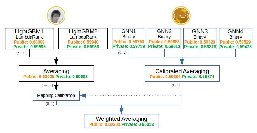\n\n## 2. LightGBM part (by Jack)\n\n### 2.1 Candidate Generation\n\nBefore I go into details, let me just say that the method described here is my own, but when I optimized Recall@20, there was little difference of performance between it and the [Chris's Public Notebook](https://www.kaggle.com/code/cdeotte/compute-validation-score-cv-565) on validation. Thus, it is unclear how much of an advantage it may have.\n\nThe basic idea is to approximate a kind of posterior probability (let's call it a candidate score) of aids based on the co-visitation matrix, and the candidates were selected from the top ones. These candidates are common to all three action types.\n\nThe last 10 aids and action types of the session were used to calculate the candidate score. That is, the score can be calculated as follows:\n\n$$Score(aid) = P(aid | (aid_1, type_1), (aid_2, type_2), ..., (aid_{10}, type_{10}))$$\n\nHere, we forcibly assume independence and conditional independence of each action, similar in concept to Naive Bayes,\n\n$$\\begin{eqnarray}\nScore(aid)\n&=& P(aid) \\cdot \\frac{P((aid_1, type_1), ..., (aid_{10}, type_{10}) | aid)}{P((aid_1, type_1), ..., (aid_{10}, type_{10}))} \\\\\\\\\n&\\approx& P(aid) \\cdot \\prod_{i=1}^{10} \\frac{P((aid_i, type_i) | aid)}{P(aid_i, type_i)} \\\\\\\\\n&=& P(aid) \\cdot \\prod_{i=1}^{10} \\frac{P((aid_i, type_i), aid)}{P(aid_i, type_i) P(aid)}\n\\end{eqnarray}$$\n\nThe term inside the product is the ratio of the joint probability to the product of individual probability, that represents the extent to which P(aid) is enhanced by the observation of (aid_i, type_i). It is quite impossible to assume the above independence with this data, and therefore this value can exceed 1 and is no longer a probability. However, I expected it to work reasonably well in prioritizing candidates.\n\nEach term in the above equation is obtained by counting the frequency of each aid and co-visitation of aid pairs and dividing by the total number of sessions. In calculating the co-visitation matrix, only interactions within a 24-hour period are counted, and no multiple counts are made within the same session. The period of calculation was the entire period including test data (in inference phase), and co-visitation in both directions was to be counted.\n\nThe co-visitation matrix does not hold for all pairs of aids, but only those that have many co-visitation for each aid. For aid pairs that are not in the co-visitation matrix, the ratio of the joint probability on the right side of the above formula is set to 1, so that they do not affect the score calculation.\n\nIn the actual calculation, the logarithm is taken and further weighted to the most recent action, as follows:\n$$Score(aid) = \\log(P(aid)) + \\sum_{i=1}^{10} \\frac{11-i}{10} \\cdot \\log \\left( \\frac{P((aid_i, type_i), aid)}{P(aid_i, type_i) P(aid)} \\right)$$\n\nMany other heuristics, such as adding pseudo counts and adjusting by action type, have been incorporated, but they are too complicated to mention here.\n\nStarting with those with the highest candidate score, the top 200 were taken for training data, the top 300 for inference of test data, and then the already visited aids were added to make the final candidates.\n\nThe recall on validation of the top 200 candidates thus obtained was as follows:\n- clicks: 0.697\n- carts: 0.559\n- orders: 0.736\n\n### 2.2 LightGBM Rerank Model\n\nThis part is not much different from the methods already shared by others. The rerank model was trained by LightGBM (LamabdaRank), and separate models were built for each action type.\n\nOn validation, the second last week of train set (truncated) was used as training data and the last week of train set (truncated) as validation data.\nWhen inference was made on the test data, a model trained on the last week's data (LightGBM1) and a model trained on the second last week's data (LightGBM2) were built, and their outputs were ensembled by simple average. Since the training data were completely swapped, I expected a reasonable ensemble effect, but in fact it seems that the effect was only slight.\n\nMost of the features are based on co-visitation matrix, but each aggregation period is separate for training, validation, and test. That is, the co-visitation matrix is created for each of the three different periods, and the features are created, so they are leakage free.\n\nThe total number of features in the final model is 344, as follows:\n- session features (32)\n - the number of all actions (1)\n - the number of each action (3)\n - the number of unique aids in the session (1)\n - the number of unique aids of (carts/orders) and the ratio to the above (4)\n - the last action type (1)\n - the last relative timestamp from the start of the test period (1)\n - the number of actions from the last of each action type to the last action of the session (3)\n - elapsed time from i-th last action (i=2, ..., 10) to the last action of the session (9)\n - revisit ratio of all aids by pair of action types (9)\n- aid features (50)\n - count of (any/buy/click/cart/order) (5)\n - exponential decay count of (any/buy/order) (3)\n - count of (any/buy/order) in last n days (n=1~7) (21)\n - count of (any/buy/order) in last n weeks (n=1~4) (12)\n - revisit count in all sessions by pair of action types (9)\n- session*aid features (12)\n - the latest action of that aid (1)\n - the number of each action of that aid (3)\n - the number of actions from last visit to that aid to the last action of the session (1)\n - elapsed time from last visit to that aid to the last action of the session (1)\n - the above two features for each action type (6)\n- co-visitation features (250)\n - the number of co-visitation of aid with aid_i (i=1, ..., 10) devided by the global count of aid_i\n - any to any (both direction/oneway) (20)\n - any to buy (both direction/oneway) (20)\n - buy to any (both direction/oneway) (20)\n - buy to buy (both direction/oneway) (20)\n - type_i to any (both direction/oneway) (20)\n - type_i to buy (both direction/oneway) (20)\n - click to click (both direction) (10)\n - click to cart (both direction) (10)\n - cart to click (both direction) (10)\n - cart to cart (both direction) (10)\n - the rank of co-visitation of aid with aid_i (i=1, ..., 10)\n - any to any (both direction) (10)\n - any to buy (both direction) (10)\n - buy to any (both direction) (10)\n - buy to buy (both direction) (10)\n - global count of aid_i (any/buy/click/cart/type_i) (50)\n\n\\* \"any\" means the action clicks or carts or orders, and \"buy\" means the action carts or orders.\n\n## 3. GNN part (by toshi_k)\n\n### 3.1 Basic Idea\n\nI considered using DL (Deep Learning) in this competition. Since the datasets are relatively simple, E2E approach of DL seemed like a desirable solution for me. Another advantage is that multi-dimensional interactions and outputs for clicks/carts/orders are easily designed as a DL model architecture.\n\nDL based recommendation was initially proposed as a kind of non-linear collaborative filtering. The typical one is training AutoEncoder model and using the reconstruction methodology to evaluate missing ratings.\n\n- Training Deep AutoEncoders for Collaborative Filtering\n - https://arxiv.org/abs/1708.01715\n\nAlthough I implemented this type of method as a prototype, it didn't work well. The number of items was so large that it made input vectors ultra sparse. It also yielded the heavy requirements of GPU memory for FC (Fully Connected) layers and made hidden layers shallower and thinner.\n\nThe disadvantage of FC layers is having weights between all combinations of aids even if most of them have nothing to do with each other. After some considerations, I figured out GNN (Graph Neural Networks) can solve this issue. The graph for GNN can represents aid relations and GNN can predict attributions of aids based on the nearly connected aids.\n\nUsing GNN for session based recommendation is also reported in the below study. According to the paper, their method is developed to explore rich transitions among items and generate accurate latent vectors of items. Their experiments on two datasets including thousands of items show that their method outperforms the state-of-the-art methods.\n\n- Session-based Recommendation with Graph Neural Networks\n - https://arxiv.org/abs/1811.00855v4\n\nMy approach is similar to the previous study. One of the biggest differences of problem setting is the number of items. In this competition, the datasets contain millions of items. To handle all items, I built a simpler workflow and installed the subgraph extraction from the global session graph.\n\nBasically, my approach has 3 steps.\n1. Construct the global graph that represents aid relations\n2. Extract the subgraph from the global graph for each session\n3. Use GNN to predict which aid will be taken\n\nThe conceptual diagram is as below.\n\n\n\nIn the first step, the global graph that represents aid relations is constructed. A subset of training data is used to create this graph. All transitions in this data are counted up and top P transitions (P=20, 30 or 40) from each aid are adopted as the edges of the graph. This graph is roughly corresponding to the co-visitation matrix that other participants call.\n\nSecondly, the subgraph is extracted from the global graph for each session. The history of each session is traced and nearly connected nodes (=aids) are listed up. Closer nodes and major transitions are prioritised and hundreds aids are filtered for extraction. This process is roughly corresponding to the candidates generation other participants call.\n\nThirdly, subgraphs are used to train and test GNN. The last layer of GNN has three channels. They predict if clicks/carts/orders will be taken in the future of each session. The inputs of GNN are the structures of subgraphs and features of nodes and edges. More details of features and GNN model are described in the next two subsections.\n\n### 3.2 Features\n\nThe input features for my GNN consist of \"node features\" and \"edge features\". Node features represent the characteristics of each aid. Edge features represent the relations between each pair of aids.\n\nBasically the total number of node features is 18. Nine of them is the global characteristics of aids. These features are shared among all sessions. The other nine features represent the history of sessions. These features are calculated on the session history and different for every sessions. The list of node features is as below.\n\n- Node features (18)\n - Global aid features (9)\n - Popularity counts (3)\n - Repeat counts (3)\n - Type transition counts (3)\n - Session history features (9)\n - Distance from the session history (2)\n - Number of counts in the session history (3)\n - Visited order features (2)\n - Visited time features (2)\n\nTotal number of edge features is 14. Twelve of them is the global characteristics of transitions. These features are shared among all sessions. The other two features represent the history of sessions. These features are calculated on the session history and different for every sessions. The list of edge features is as below.\n\n- Edge features (14)\n - Global transition features (12)\n - Transition count not considering types (2)\n - Transition rank not considering types (2)\n - Cart-to-cart transition count (2)\n - Cart-to-cart transition rank (2)\n - Order-to-order transition count (2)\n - Order-to-order transition rank (2)\n - Session history features (2)\n - Self loop or not (1)\n - Stepped in session history or not (1)\n\nAny combinations of multiple features and higher dimension features are not added. It was expected that such complex features were automatically captured by the representation capability of GNN.\n\nAll missing values are filled with zero and logarithmic transformation (log1p) is applied to most features for the stability of GNN.\n\n### 3.3 Model and Loss function\n\nMy GNN has 8 GCN (Graph Convolution) layers. This implies GNN model can consider aids located within 8 steps from the history aids for prediction. In some trial experiments, 8 layers model was better than 4 layers one a little, but it was unclear more layers helped or not. \n\nAside from GCN layers, my model employs non linear activation functions, skip connections, and normalization layers. These component made training faster and yielded less training loss.\n\nAs mentioned above, the last layer has three channels for clicks/carts/orders. The channels for carts and orders are connected with sigmoid functions and trained by binary cross entropy loss. The channel for clicks is connected with softmax function and trained by softmax cross entropy loss.\n\n### 3.4 Performance boosting\n\nI noticed that increasing the number of candidates for inference boosted the LB score. For example, my best model improved from 0.59474 to 0.59750 on public LB by increasing the candidates from 384 to 1024.\n\n| Model | num of candidates | Public LB | Private LB |\n| --- | --- | --- | --- |\n| Model1 | 384 | 0.59474 | 0.59451 | \n| Model1 | 1024 | 0.59750 | 0.59719 |\n\nUnfortunately, more candidates required more computational calculation, 1024 candidates took several days for inference. I increased candidates as much as possible and save the outputs of several models.\n\nAs the final stage of the competition, ensemble of multiple predictions is attempted. Four GNN models are used for this ensemble. Although they were trained with slightly different setting, their basic approaches were the same. Ensemble of 4 models achieved 0.59894 on public LB and 0.59874 on private LB.\n\n| Model | num of candidates | Public LB | Private LB |\n| --- | --- | --- | --- |\n| Model1 | 1024 | 0.59750 | 0.59719 | \n| Model2 | 1024 | 0.59653 | 0.59613 |\n| Model3 | 512 | 0.59320 | 0.59318 |\n| Model4 | 768 | 0.59529 | 0.59478 |\n| Ensemble of 4 models | - | 0.59894 | 0.59874 |\n\n## 4. Team Ensemble (by toshi_k)\n\nAfter we made up a team, we tried several ways to merge our predictions. We started from the simple rerank by arithmetic mean of ranks in submission files. It improved the public score 0.597→0.600 then.\n\nThe next attempt was using raw prediction to boost LB score more. We saved the raw prediction of top 50 aids of each part. The biggest issue was the outputs from LambdaRank range in any real number while the output of GNN range in (0, 1).\n\nSince we didn't have enough time to lead the best theoretical way, we tried some ensemble method experimentally. One interesting finding was the logit transformed value of GNN seemed to have the proportional relationship with LambdaRank with constant shift.\n\n$$ \\mathrm{logit}(p^\\text{Binary Prediction}) \\propto v^\\text{LambdaRank prediction} + C $$\n\nThe value of constant shift is different on every session_types. This may be just a brute force approximation, we estimate C for each session_type and mapped the output of LambdaRank to 0-to-1 value.\n\n$$\\begin{eqnarray}\n\\hat{C} &=& \\arg \\min_C \\\\{ \\frac{1}{R} \\sum_r^R {^Gp_r} - \\frac{1}{R} \\sum_r^R \\sigma(^Lv_r + C) \\\\}^2 \\\\\\\\\n^Lp_r &=& \\sigma (v^L_r + \\hat{C}) \\\\\\\\\n\\mathrm{where:} \\\\\\\\\n^Gp_r &=& \\text{rth output of GNN} \\in (0, 1) \\\\\\\\\\\\\n^Lv_r &=& \\text{rth output of LambdaRank LGBM } \\in \\mathbb{R} \\\\\\\\\\\\\n^Lp_r &=& \\text{0-1 calibrated value of } ^Lv_r \\in (0, 1)\n\\end{eqnarray}$$\n\nAfter this transformation, simple weighted averaging was calculated. Since LightGBM part achieved better score on PublicLB, the weight of LightGBM is set to be larger than GNN part. We tried two patterns of weight settings and chose both of them as final submissions.\n\n| | weight | Public LB | Private LB |\n| --- | --- | --- | --- |\n| LightGBM Part | 1.000 (LightGBM) : 0.000 (GNN) | 0.60025 | 0.60008 | \n| GNN part | 0.000 (LightGBM) : 1.000 (GNN) | 0.59894 | 0.59874 | \n| Final Submission 1 | 0.600 (LightGBM) : 0.400 (GNN) | 0.60311 | 0.60307 | \n| Final Submission 2 | 0.525 (LightGBM) : 0.475 (GNN) | 0.60302 | 0.60313 |\n\nBoth of final submissions improved LB score from the best of two parts. While Final Submission 1 was the best on public LB, Final Submission 2 was the best on private LB. Even though all single models got worse on private LB, the score of Final Submission 2 on private LB is better than public LB. Out team merge and ensemble was successful in this sense.\n\n## 5. Conclusion\n\nOur team employed LightGBM and GNN for this competition. Each approach took different way for candidate generation, feature engineering and model design. Ensemble of two types of approaches boosted our team score a lot.\n\nThis competition gave 6th gold model to toshi_k and 7th gold to Jack. It motivate us for the further success. What we learn in this competition can be applied to not only future competitions but real world projects. It was confirmed that Kaggle is the practical platform of data science again.\n\nThank you for reading this to the end!", "votes": null }, { "id": "2130095", "postDate": "02/05/2023 06:16:01", "content": "Fantastic result and great approach note @rsakata! All the best and best regards!
", "rawMarkdown": "Fantastic result and great approach note @rsakata! All the best and best regards!", "votes": null }, { "id": "2130310", "postDate": "02/05/2023 11:03:35", "content": "@toshik Congratulation for gold medals. I think gold medals of this tough competition has special values.
\nI have a question, about ensemble of each single GNN models, what “calibrated average” actually calculates?
\nAlso, since I’m not familiar with this technique, I will appreciate if you share some references if any.
Thank you for sharing this unique & special approach. Although I don’t understand all the specifics, I guess utilizing GNN as such extent requires deep understanding of this literature.
", "rawMarkdown": "toshik Congratulation for gold medals. I think gold medals of this tough competition has special values.\n\nI have a question, about ensemble of each single GNN models, what “calibrated average” actually calculates?\nAlso, since I’m not familiar with this technique, I will appreciate if you share some references if any.\n\nThank you for sharing this unique & special approach. Although I don’t understand all the specifics, I guess utilizing GNN as such extent requires deep understanding of this literature.", "votes": null }, { "id": "2130516", "postDate": "02/05/2023 14:00:24", "content": "@tatamikenn Thank you for your comment. I'm not ready to share details of that part, but It was just a trivial technique. When some of my models output confident values (e.g. 0.4-1.0) and the others output less confident values (e.g. 0.0-0.6), they are calibrated to the same range (e.g 0.2-0.8) before averaging.
", "rawMarkdown": "tatamikenn Thank you for your comment. I'm not ready to share details of that part, but It was just a trivial technique. When some of my models output confident values (e.g. 0.4-1.0) and the others output less confident values (e.g. 0.0-0.6), they are calibrated to the same range (e.g 0.2-0.8) before averaging.", "votes": null }, { "id": "2130675", "postDate": "02/05/2023 16:08:29", "content": "Thank you for sharing very useful content.
", "rawMarkdown": "Thank you for sharing very useful content.", "votes": null }, { "id": "2130798", "postDate": "02/05/2023 17:35:26", "content": "Great ! What did you use to train the GNN ? I thought it requires a lot of resources and should be slower to train. I personally used an heterogenous graph but I could use only kaggle kernels. I build a kind of GCN Autoencoder by reconstructing the adjacency matrix and then:
\nNow I think that I should used it to extract other candidates ( another matrix ) to improve my classifications k by providing potential more true positives.
\nThanks for your great topic !
", "rawMarkdown": "Great ! What did you use to train the GNN ? I thought it requires a lot of resources and should be slower to train. I personally used an heterogenous graph but I could use only kaggle kernels. I build a kind of GCN Autoencoder by reconstructing the adjacency matrix and then:\n- use the encoding of both entities as features.\n- apply a KNN Graph on the Users Embeddings to extract the nearest K AIDs.\n\nNow I think that I should used it to extract other candidates ( another matrix ) to improve my classifications k by providing potential more true positives.\n\nThanks for your great topic !", "votes": null }, { "id": "2130866", "postDate": "02/05/2023 18:31:38", "content": "This is brilliant - congratulations both of you! 🎉 It's so interesting to see such an in-depth explanation of a GNN approach to this competition, and great to see the boost in performance you got from ensembling the two methods together :)
", "rawMarkdown": "This is brilliant - congratulations both of you! 🎉 It's so interesting to see such an in-depth explanation of a GNN approach to this competition, and great to see the boost in performance you got from ensembling the two methods together :)", "votes": null }, { "id": "2132075", "postDate": "02/06/2023 15:35:33", "content": "Thats amazing. Using GNN approach to solve this !!
", "rawMarkdown": "Thats amazing. Using GNN approach to solve this !!", "votes": null }, { "id": "2132671", "postDate": "02/07/2023 01:26:00", "content": "@rayanaay My machine has Core-i9 10980XE and RTX A6000. It was actually resource consuming to train models. Although using GCN autoencoder may be a possible approach, extract candidates and ML based reranking would be important regardless of whether it is used.
", "rawMarkdown": "rayanaay My machine has Core-i9 10980XE and RTX A6000. It was actually resource consuming to train models. Although using GCN autoencoder may be a possible approach, extract candidates and ML based reranking would be important regardless of whether it is used.", "votes": null }, { "id": "2134525", "postDate": "02/08/2023 03:56:22", "content": "Amazing result!!
\n@toshik Could you share your gnn training/inference code?
Your solution is quite unique and well thought out, combining the strengths of both LightGBM and GNN. @rsakata your candidate generation approach is quite impressive, utilizing the co-visitation matrix and a posterior probability approximation to prioritize the candidate aids. And @toshik your use of GNN to handle the large number of items in the datasets is very clever and effective, especially with the added step of subgraph extraction from the global session graph.
\n@toshik @rsakata I have a few questions regarding your solution:
\n@giranntu The subgraph extraction step helps the model to focus on prospective items. While processing whole graph on GPU is impossible due to the memory limitation, subgraphs can be processed on GPU.
\nI tuned hyperparameters manually. Hyperparameters tuning for GNN is so severe that defining search configuration is still difficult.
Fantastic result and great approach note @rsakata! All the best and best regards!
", "votes": null, "replies": [] }, { "id": 2130310, "author_name": "tatamikenn", "author_url": "", "post_date": "02/05/2023 11:03:35", "content": "@toshik Congratulation for gold medals. I think gold medals of this tough competition has special values.
\nI have a question, about ensemble of each single GNN models, what “calibrated average” actually calculates?
\nAlso, since I’m not familiar with this technique, I will appreciate if you share some references if any.
Thank you for sharing this unique & special approach. Although I don’t understand all the specifics, I guess utilizing GNN as such extent requires deep understanding of this literature.
", "votes": null, "replies": [ { "id": 2130516, "author_name": "toshik", "author_url": "", "post_date": "02/05/2023 14:00:24", "content": "@tatamikenn Thank you for your comment. I'm not ready to share details of that part, but It was just a trivial technique. When some of my models output confident values (e.g. 0.4-1.0) and the others output less confident values (e.g. 0.0-0.6), they are calibrated to the same range (e.g 0.2-0.8) before averaging.
", "votes": null, "replies": [] } ] }, { "id": 2130675, "author_name": "ibrahimkaratas", "author_url": "", "post_date": "02/05/2023 16:08:29", "content": "Thank you for sharing very useful content.
", "votes": null, "replies": [] }, { "id": 2130798, "author_name": "rayanaay", "author_url": "", "post_date": "02/05/2023 17:35:26", "content": "Great ! What did you use to train the GNN ? I thought it requires a lot of resources and should be slower to train. I personally used an heterogenous graph but I could use only kaggle kernels. I build a kind of GCN Autoencoder by reconstructing the adjacency matrix and then:
\nNow I think that I should used it to extract other candidates ( another matrix ) to improve my classifications k by providing potential more true positives.
\nThanks for your great topic !
", "votes": null, "replies": [ { "id": 2132671, "author_name": "toshik", "author_url": "", "post_date": "02/07/2023 01:26:00", "content": "@rayanaay My machine has Core-i9 10980XE and RTX A6000. It was actually resource consuming to train models. Although using GCN autoencoder may be a possible approach, extract candidates and ML based reranking would be important regardless of whether it is used.
", "votes": null, "replies": [] } ] }, { "id": 2130866, "author_name": "judehunt23", "author_url": "", "post_date": "02/05/2023 18:31:38", "content": "This is brilliant - congratulations both of you! 🎉 It's so interesting to see such an in-depth explanation of a GNN approach to this competition, and great to see the boost in performance you got from ensembling the two methods together :)
", "votes": null, "replies": [] }, { "id": 2132075, "author_name": "sohilsharma1996", "author_url": "", "post_date": "02/06/2023 15:35:33", "content": "Thats amazing. Using GNN approach to solve this !!
", "votes": null, "replies": [] }, { "id": 2134525, "author_name": "no9more9ria10", "author_url": "", "post_date": "02/08/2023 03:56:22", "content": "Amazing result!!
\n@toshik Could you share your gnn training/inference code?
Your solution is quite unique and well thought out, combining the strengths of both LightGBM and GNN. @rsakata your candidate generation approach is quite impressive, utilizing the co-visitation matrix and a posterior probability approximation to prioritize the candidate aids. And @toshik your use of GNN to handle the large number of items in the datasets is very clever and effective, especially with the added step of subgraph extraction from the global session graph.
\n@toshik @rsakata I have a few questions regarding your solution:
\n@giranntu The subgraph extraction step helps the model to focus on prospective items. While processing whole graph on GPU is impossible due to the memory limitation, subgraphs can be processed on GPU.
\nI tuned hyperparameters manually. Hyperparameters tuning for GNN is so severe that defining search configuration is still difficult.