{"cells":[{"metadata":{},"cell_type":"markdown","source":"## Introduction\n\n### [What is Pulmonary Fibrosis?](https://www.mayoclinic.org/diseases-conditions/pulmonary-fibrosis/symptoms-causes/syc-20353690)\n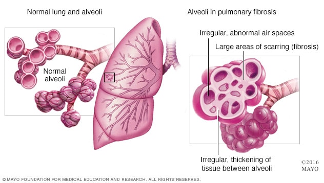\n* Pulmonary fibrosis is lung disease that occurs when the lung tissues become thick ans scarred. As a result, breathing becomes progressively more difficult for the patient suffering from the disease.\n* The disease may be progressing a someone's body for a long time without any warning. And then suddenly symptoms show up and can make a patient much worse.\n\n### [Causes](https://en.wikipedia.org/wiki/Pulmonary_fibrosis#Cause)\n* Most of the time, it is difficult to find the cause. And in such cases it is termed as idiopathic pulmonary fibrosis.\n* Pulmonary fibrosis can be a secondary effect to other diseases as well. Examples include autoimmune disorders, viral infections and bacterial infection like tuberculosis which may cause fibrotic changes in both lung's upper or lower lobes and other microscopic injuries to the lung ([Source](https://en.wikipedia.org/wiki/Pulmonary_fibrosis#Cause)).\n* The following image shows an chest x-ray with pulmonary fibrosis ([Source](https://en.wikipedia.org/wiki/Pulmonary_fibrosis#Cause)).\n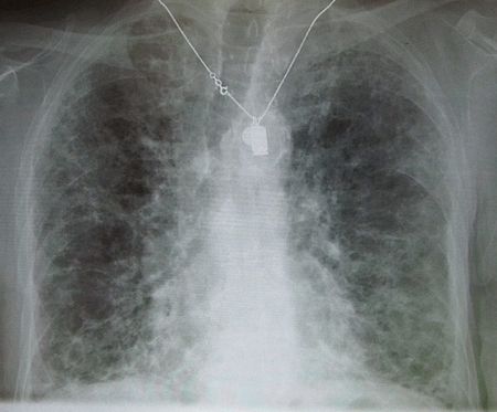\n* The following image is an HRCT of lung showing extensive fibrosis ([Source](https://en.wikipedia.org/wiki/File:Pulmon_fibrosis.PNG))\n\n\n### Symptoms\n* The following are the symptoms of pulmoary fibrosis ([Source](https://en.wikipedia.org/wiki/Pulmonary_fibrosis#Signs_and_symptoms)).\n * Shortness of breath, particularly with exertion.\n * Chronic dry, hacking coughing.\n * Fatigue and weakness.\n * Chest discomfort including chest pain.\n * Loss of appetite and rapid weight loss.","execution_count":null},{"metadata":{},"cell_type":"markdown","source":"## The Aim of This Competition\nIn this competition, we’ll predict a patient’s severity of decline in lung function based on a CT scan of their lungs. We’ll determine lung function based on output from a spirometer, which measures the volume of air inhaled and exhaled. The challenge is to use machine learning techniques to make a prediction with the image, metadata, and baseline FVC as input.\n\n* **Now let's move ahead and explore the data that is given to us in this competition**.\n\n### Evaluation Metric\nThis competition is evaluated on a modified version of the Laplace Log Likelihood. In medical applications, it is useful to evaluate a model's confidence in its decisions. Accordingly, the metric is designed to reflect both the accuracy and certainty of each prediction.\n\n#### What is FVC?\nLung function is assessed based on output from a spirometer, which measures the forced vital capacity (FVC), i.e. the volume of air exhaled.\n\n\nFor each true FVC measurement, we will predict both an FVC and a confidence measure (standard deviation σ). The metric is computed as:\n\n$$\\sigma_{clipped} = max(\\sigma, 70)$$\n$$\\Delta = min ( |FVC_{true} - FVC_{predicted}|, 1000 )$$\n$$metric = - \\frac{\\sqrt{2} \\Delta}{\\sigma_{clipped}} - \\ln ( \\sqrt{2} \\sigma_{clipped} )$$","execution_count":null},{"metadata":{"_uuid":"8f2839f25d086af736a60e9eeb907d3b93b6e0e5","_cell_guid":"b1076dfc-b9ad-4769-8c92-a6c4dae69d19","trusted":true},"cell_type":"code","source":"import pydicom\nimport pandas as pd\nimport matplotlib.pyplot as plt\nimport matplotlib\nimport seaborn as sns\n\nmatplotlib.style.use('ggplot')","execution_count":null,"outputs":[]},{"metadata":{"_uuid":"d629ff2d2480ee46fbb7e2d37f6b5fab8052498a","_cell_guid":"79c7e3d0-c299-4dcb-8224-4455121ee9b0","trusted":true},"cell_type":"code","source":"DIR_ROOT = '../input/osic-pulmonary-fibrosis-progression'\n\ntrain_csv = pd.read_csv(f\"{DIR_ROOT}/train.csv\")","execution_count":null,"outputs":[]},{"metadata":{},"cell_type":"markdown","source":"## Taking a Look at Patient Data","execution_count":null},{"metadata":{"trusted":true},"cell_type":"code","source":"train_csv.head()","execution_count":null,"outputs":[]},{"metadata":{"trusted":true},"cell_type":"code","source":"print(f\"Total number of patient IDs: {len(train_csv)}\")","execution_count":null,"outputs":[]},{"metadata":{"trusted":true},"cell_type":"code","source":"train_csv.info()","execution_count":null,"outputs":[]},{"metadata":{"trusted":true},"cell_type":"code","source":"train_csv.describe()","execution_count":null,"outputs":[]},{"metadata":{"trusted":true},"cell_type":"code","source":"train_csv.isnull().values.any()","execution_count":null,"outputs":[]},{"metadata":{},"cell_type":"markdown","source":"So, we do not have any NaN values in the dataset. That means, we can peacefully move on to the EDA part of this notebook.","execution_count":null},{"metadata":{},"cell_type":"markdown","source":"There are 1549 patient IDs in the CSV file. But all the IDs are not unique. This means that a patient might have returned after 2 years of the first scan and then may been given a new unique ID.","execution_count":null},{"metadata":{"trusted":true},"cell_type":"code","source":"print(train_csv.Patient.value_counts())\nprint(train_csv.Patient.value_counts().keys())\npatient_id_keys = [train_csv.Patient.value_counts()]\n# print(patient_id_keys)","execution_count":null,"outputs":[]},{"metadata":{},"cell_type":"markdown","source":"So, there are 176 unique patent IDs. Let's plot these out.","execution_count":null},{"metadata":{"trusted":true},"cell_type":"code","source":"patient_id_dict = {'id': [], 'num': []}\npatient_keys = train_csv.Patient.value_counts().keys()\nfor i, data in enumerate(train_csv.Patient.value_counts()):\n patient_id_dict['id'].append(patient_keys[i])\n patient_id_dict['num'].append(data)","execution_count":null,"outputs":[]},{"metadata":{"trusted":true},"cell_type":"code","source":"plt.figure(figsize=(20, 17))\nplt.bar(patient_id_dict['id'], patient_id_dict['num'], color='orange')\nplt.tick_params(\n axis='x', \n which='both', \n bottom=False, \n top=False, \n labelbottom=False) \nplt.show()","execution_count":null,"outputs":[]},{"metadata":{},"cell_type":"markdown","source":"The above plot does not look very clean. Now we know that the highest of times a patient has visited according to the dataset is 10, and the lowest number of 6. What we can do is visualize how many patients visited a particualr number of time starting from 10 to 6.","execution_count":null},{"metadata":{"trusted":true},"cell_type":"code","source":"num_patients_list = []\nnum_visits = []\nfor i in range(10, 5, -1):\n num_visits.append(i)\n num_patients_counter = 0\n for j in range(len(train_csv.Patient.value_counts())):\n if i == patient_id_dict['num'][j]:\n num_patients_counter += 1\n num_patients_list.append(num_patients_counter)","execution_count":null,"outputs":[]},{"metadata":{"trusted":true},"cell_type":"code","source":"plt.figure(figsize=(10, 7))\nplt.bar(num_patients_list, num_visits, color='orange', width=1)\nplt.xlabel('Number of patients')\nplt.ylabel('Number of times visited')\nplt.show()","execution_count":null,"outputs":[]},{"metadata":{},"cell_type":"markdown","source":"So, it looks like 10 patients visited the most number of times, that is 10 times. And around 150 patients visited 9 times. ","execution_count":null},{"metadata":{},"cell_type":"markdown","source":"### Grouping by Patient ID\nWe already know that we have 176 patients. So, we can group by patient ID and check all the valuable information. Maybe that will lead to some useful information and visualtion.","execution_count":null},{"metadata":{"trusted":true},"cell_type":"code","source":"mean_csv = train_csv.groupby(['Patient']).mean()\nprint(mean_csv.head())\nprint(mean_csv.columns)","execution_count":null,"outputs":[]},{"metadata":{},"cell_type":"markdown","source":"From the above information, we plot a lot of things inlcuding:\n* Mean number of weeks a patient has visited.\n* Mean FVC of each patient.\n* Mean FVC percentage in accordance with other patients with similar symptoms.\n* The age of each patient.","execution_count":null},{"metadata":{},"cell_type":"markdown","source":"#### Number of Weeks Visited by The Patients","execution_count":null},{"metadata":{"trusted":true},"cell_type":"code","source":"plt.figure(figsize=(15, 12))\nsns.scatterplot(patient_id_dict['id'], mean_csv['Weeks'], \n hue=mean_csv['Weeks'], size=mean_csv['Weeks'], \n sizes=(10, 200))\nplt.tick_params(\n axis='x', \n which='both', \n bottom=False, \n top=False, \n labelbottom=False) ","execution_count":null,"outputs":[]},{"metadata":{},"cell_type":"markdown","source":"From the above plot we can easily infer that most patients visited somewhere within 20 to 30 weeks. There are a few outliers and only one patients visited more than 80 times for the Pulmonary Fibrosis treatment.","execution_count":null},{"metadata":{},"cell_type":"markdown","source":"#### Mean FVC of Each Patient","execution_count":null},{"metadata":{"trusted":true},"cell_type":"code","source":"plt.figure(figsize=(18, 15))\nsns.barplot(patient_id_dict['id'], mean_csv['FVC'])\nplt.ylabel('Mean FVC (in ml)')\nplt.tick_params(\n axis='x', \n which='both', \n bottom=False, \n top=False, \n labelbottom=False) ","execution_count":null,"outputs":[]},{"metadata":{},"cell_type":"markdown","source":"#### Mean FVC Percentage of Each Patient","execution_count":null},{"metadata":{"trusted":true},"cell_type":"code","source":"plt.figure(figsize=(18, 15))\nsns.barplot(patient_id_dict['id'], mean_csv['Percent'], \n palette=\"rocket\")\nplt.ylabel('FVC Perncentage')\nplt.tick_params(\n axis='x', \n which='both', \n bottom=False, \n top=False, \n labelbottom=False) ","execution_count":null,"outputs":[]},{"metadata":{},"cell_type":"markdown","source":"#### Age of Each Patient","execution_count":null},{"metadata":{"trusted":true},"cell_type":"code","source":"plt.figure(figsize=(15, 12))\nsns.swarmplot(patient_id_dict['id'], mean_csv['Age'])\nplt.ylabel('Age')\nplt.tick_params(\n axis='x', \n which='both', \n bottom=False, \n top=False, \n labelbottom=False) ","execution_count":null,"outputs":[]},{"metadata":{},"cell_type":"markdown","source":"The above swarm plot shows that most of the people are aged between 63 and 73. Few people below the age of 60 are suffering from Pulomonaru Fibrosis. The same is true for peole above the age of 80 as well.","execution_count":null},{"metadata":{},"cell_type":"markdown","source":"**I hope that you liked this basic EDA. A lot more can be done with the data that we have at hand. But for now, it's time to build some deep learning models.**","execution_count":null},{"metadata":{"trusted":true},"cell_type":"code","source":"","execution_count":null,"outputs":[]}],"metadata":{"kernelspec":{"language":"python","display_name":"Python 3","name":"python3"},"language_info":{"pygments_lexer":"ipython3","nbconvert_exporter":"python","version":"3.6.4","file_extension":".py","codemirror_mode":{"name":"ipython","version":3},"name":"python","mimetype":"text/x-python"}},"nbformat":4,"nbformat_minor":4}