{"cells":[{"metadata":{},"cell_type":"markdown","source":"#      👨‍⚕️ _OSIC Pulmonary Fibrosis Progression_ 👩‍⚕️ ","execution_count":null},{"metadata":{},"cell_type":"markdown","source":"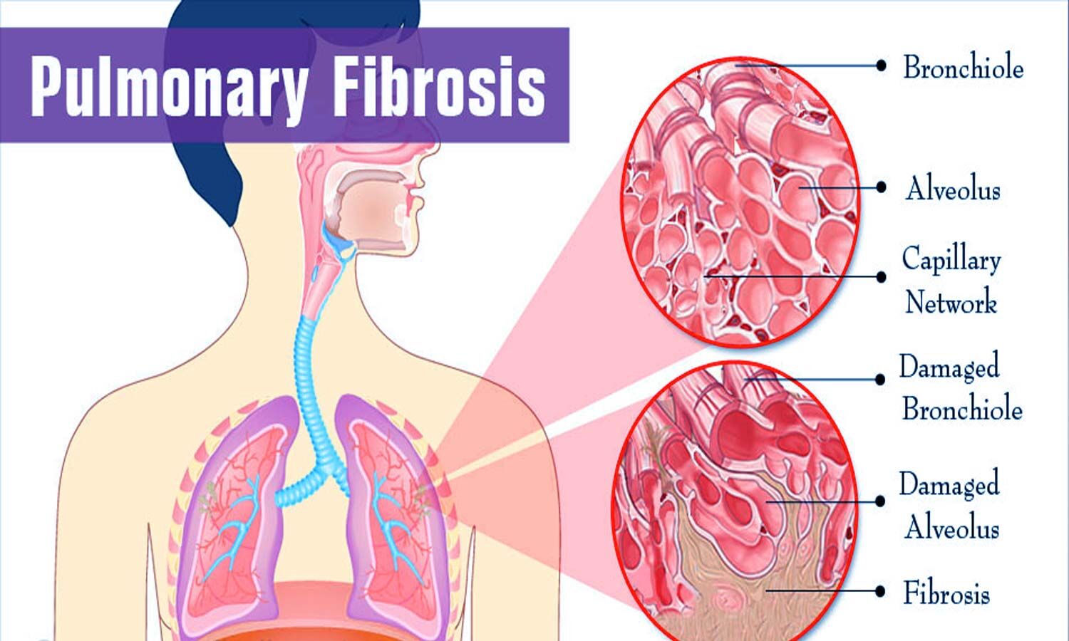![](https://medicaldialogues.in/h-upload/2020/05/18/128958-idiopathic-pulmonary-fibrosis.jpg)","execution_count":null},{"metadata":{},"cell_type":"markdown","source":"# <font color='red'>1. Introduction</font> 👨🏻‍💻\n## _1.1 What is Pulmonary Fibrosis ?_","execution_count":null},{"metadata":{},"cell_type":"markdown","source":"Pulmonary fibrosis is a lung disease that occurs when lung tissue becomes damaged and scarred. This thickened, stiff tissue makes it more difficult for your lungs to work properly. As pulmonary fibrosis worsens, you become progressively more short of breath.","execution_count":null},{"metadata":{},"cell_type":"markdown","source":"## _1.2 About OSIC :_ \n***Open Source Imaging Consortium*** (OSIC) is a not-for-profit, co-operative effort between academia, industry and philanthropy. The group enables rapid advances in the fight against Idiopathic Pulmonary Fibrosis (IPF), fibrosing interstitial lung diseases (ILDs), and other respiratory diseases, including emphysematous conditions.","execution_count":null},{"metadata":{},"cell_type":"markdown","source":"## _1.3 Competition Objective :_\n\nIn this competition, you’ll predict a patient’s severity of decline in lung function based on a CT scan of their lungs. You’ll determine lung function based on output from a spirometer, which measures the volume of air inhaled and exhaled. The challenge is to use machine learning techniques to make a prediction with the image, metadata, and baseline FVC as input.","execution_count":null},{"metadata":{},"cell_type":"markdown","source":"## _1.4 Evaluation Metric :_\n**Laplace Log Likelihood (modified version)**: useful to evaluate a model's confidence in its decisions. Accordingly, the metric is designed to reflect both the accuracy and certainty of each prediction.\n\n\nThe error is thresholded at 1000 ml to avoid large errors adversely penalizing results, while the confidence values are clipped at 70 ml to reflect the approximate measurement uncertainty in FVC. \n\n<font color='red'>Note : The metric values will be negative and higher is better.</font>","execution_count":null},{"metadata":{},"cell_type":"markdown","source":"## _1.5 Importing relevant packages_ 📦","execution_count":null},{"metadata":{"_uuid":"8f2839f25d086af736a60e9eeb907d3b93b6e0e5","_cell_guid":"b1076dfc-b9ad-4769-8c92-a6c4dae69d19","trusted":true},"cell_type":"code","source":"import os\nimport cv2\nimport plotly\nimport pydicom\nimport numpy as np\nimport pandas as pd\nimport seaborn as sns\nimport plotly.express as px\nimport matplotlib.pyplot as plt\nimport plotly.graph_objects as go\nimport plotly.figure_factory as ff\nimport plotly.graph_objs as go\nfrom plotly.subplots import make_subplots\nfrom plotly.offline import init_notebook_mode, iplot\ninit_notebook_mode(connected = True)\n\nfrom IPython.display import display_html\nfrom PIL import Image\nimport gc\nfrom scipy.stats import pearsonr\nimport pydicom # for DICOM images\nfrom skimage.transform import resize\nimport copy\nimport re\n\n# Segmentation\nfrom glob import glob\nfrom mpl_toolkits.mplot3d.art3d import Poly3DCollection\nimport scipy.ndimage\nfrom skimage import morphology\nfrom skimage import measure\nfrom skimage.transform import resize\nfrom sklearn.cluster import KMeans\nfrom plotly import __version__\nfrom plotly.offline import download_plotlyjs, init_notebook_mode, plot, iplot\nfrom plotly.tools import FigureFactory as FF\nfrom plotly.graph_objs import *\ninit_notebook_mode(connected=True) \n\nimport warnings\nwarnings.filterwarnings(\"ignore\")\n\n# Set Color Palettes for the notebook\ncustom_colors = ['#74a09e','#86c1b2','#98e2c6','#f3c969','#f2a553', '#d96548', '#c14953']","execution_count":null,"outputs":[]},{"metadata":{},"cell_type":"markdown","source":"## _1.6 Importing the train and test set ..._ 🧪","execution_count":null},{"metadata":{"_uuid":"d629ff2d2480ee46fbb7e2d37f6b5fab8052498a","_cell_guid":"79c7e3d0-c299-4dcb-8224-4455121ee9b0","trusted":true},"cell_type":"code","source":"train = pd.read_csv('../input/osic-pulmonary-fibrosis-progression/train.csv')\ntrain.head()","execution_count":null,"outputs":[]},{"metadata":{"trusted":true},"cell_type":"code","source":"test = pd.read_csv('../input/osic-pulmonary-fibrosis-progression/test.csv')\ntest.head()","execution_count":null,"outputs":[]},{"metadata":{},"cell_type":"markdown","source":"#### **We see that there are 7 features in each train and test sets. Let's look at what each feature means :**\n- **Patient** - a unique Id for each patient (also the name of the patient's DICOM folder)\n- **Weeks** - the relative number of weeks pre/post the baseline CT (may be negative)\n- **FVC** - the recorded lung capacity in ml (Forced vital capacity)\n- **Percent** - a computed field which approximates the patient's FVC as a percent of the typical FVC for a person of similar characteristics\n- **Age** - Age of person\n- **Sex** - Sex of person (Male/Female)\n- **SmokingStatus** - Whether the patient is a smoker/non-smoker/ex-smoker","execution_count":null},{"metadata":{},"cell_type":"markdown","source":"### _1.6.1 Dimensions of our dataset_","execution_count":null},{"metadata":{"trusted":true},"cell_type":"code","source":"print(\"Shape of training set : {}\".format(train.shape))\nprint(\"Shape of testing set : {}\".format(test.shape))","execution_count":null,"outputs":[]},{"metadata":{},"cell_type":"markdown","source":"# _<font color='red'>2. Exploratory Data Analysis (EDA)</font>_ 📊","execution_count":null},{"metadata":{"trusted":true},"cell_type":"code","source":"train.info()","execution_count":null,"outputs":[]},{"metadata":{},"cell_type":"markdown","source":"The above block tells us that there are:\n- 1 float64 feature.\n- 3 int64 features.\n- 3 object type features.\n\n**It also tells us the there is no missing data from the train set as the shape of dataset is equal to the count of non-null values present in each feature.** ","execution_count":null},{"metadata":{},"cell_type":"markdown","source":"### But just to make sure, let's check if there is any missing data...","execution_count":null},{"metadata":{"trusted":true},"cell_type":"code","source":"print(\"*** Train set ***\")\nprint(train.isnull().sum())\nprint(\"--------------\")\nprint(\"*** Test set ***\")\nprint(test.isnull().sum())","execution_count":null,"outputs":[]},{"metadata":{},"cell_type":"markdown","source":"**Thus, no missing data throughout our train and test set**","execution_count":null},{"metadata":{},"cell_type":"markdown","source":"### _2.1 Descriptive Statistics_","execution_count":null},{"metadata":{"trusted":true},"cell_type":"code","source":"train.describe()","execution_count":null,"outputs":[]},{"metadata":{},"cell_type":"markdown","source":"### _2.2 No. of unique patients, Age and Smoking Status_","execution_count":null},{"metadata":{"trusted":true},"cell_type":"code","source":"print(\"Q. How many patients are present in train set ?\")\nprint(\"A.\",train['Patient'].nunique())\nprint(\"------------\")\nprint(\"Q. How many unique ages are present in train set ?\")\nprint(\"A.\",train['Age'].nunique())\nprint(\"------------\")\nprint(\"Q. How many smoking statuses are present in train set ?\")\nprint(\"A.\",train['SmokingStatus'].nunique())","execution_count":null,"outputs":[]},{"metadata":{"trusted":true},"cell_type":"markdown","source":"### _2.3 How 'FVC', 'Percent' and 'Age' are distributed_","execution_count":null},{"metadata":{"trusted":true},"cell_type":"code","source":"fig, axes = plt.subplots(1, 3, figsize=(17,5))\nfig.suptitle('Distribution of different features')\n\nsns.distplot(train['FVC'], color='blue', ax=axes[0])\nsns.distplot(train['Percent'], color='orange', ax=axes[1])\nsns.distplot(train['Age'],color='green', ax=axes[2])\n\nplt.show()","execution_count":null,"outputs":[]},{"metadata":{},"cell_type":"markdown","source":"**It is good to see that the distribution is somewhat normally distributed with a little bit of skewness for the 3 features.**","execution_count":null},{"metadata":{},"cell_type":"markdown","source":"### _2.4 Let's now have a look at the count and percentage of each - 'Sex' and 'SmokingStatus'_","execution_count":null},{"metadata":{"trusted":true},"cell_type":"code","source":"# Count of unique entities in both 'Sex' and 'SmokingStatus'\n\nsex_count = train['Sex'].value_counts()\nprint('*** Sex Count ***\\n')\nprint(\"No. of records for males in train set : {}\".format(sex_count[0]))\nprint(\"No. of records for females in train set : {}\".format(sex_count[1]))\n\nsmoker_count = train['SmokingStatus'].value_counts()\nprint(\"\\n*** Smoker's Count ***\\n\")\nprint(\"No. of records for ex-smokers in train set : {}\".format(smoker_count[0]))\nprint(\"No. of records for non-smokers in train set : {}\".format(smoker_count[1]))\nprint(\"No. of records for current smokers in train set : {}\".format(smoker_count[2]))","execution_count":null,"outputs":[]},{"metadata":{"trusted":true},"cell_type":"code","source":"fig, axes = plt.subplots(1, 2, figsize=(15,5))\nfig.suptitle(\"Count Plots\")\nsns.countplot(x='Sex', data=train, ax=axes[0])\nsns.countplot(x='SmokingStatus', data=train, ax=axes[1])\nplt.show()","execution_count":null,"outputs":[]},{"metadata":{"trusted":true},"cell_type":"code","source":"# Percentage of unique entities in both 'Sex' and 'SmokingStatus'\n\nsex_count = train['Sex'].value_counts()\nprint('*** Sex Percentage ***\\n')\nprint(\"Percentage of males in train set : {:.2f}%\".format((sex_count[0] / sex_count.sum()) * 100))\nprint(\"Percentage of females in train set : {:.2f}%\".format((sex_count[1] / sex_count.sum()) * 100))\n\nsmoker_count = train['SmokingStatus'].value_counts()\nprint(\"\\n*** Smoker's Percentage ***\\n\")\nprint(\"Percentage of ex-smokers in train set : {:.2f}%\".format((smoker_count[0] / smoker_count.sum()) * 100))\nprint(\"Percentage of non-smokers in train set : {:.2f}%\".format((smoker_count[1] / smoker_count.sum()) * 100))\nprint(\"Percentage of current smokers in train set : {:.2f}%\".format((smoker_count[2] / smoker_count.sum()) * 100))","execution_count":null,"outputs":[]},{"metadata":{"trusted":true},"cell_type":"code","source":"labels1 = ['Male', 'Female']\nvalues1 = [sex_count[0], sex_count[1]]\nlabels2 = ['Ex-smokers', 'Never Smoked', 'Current Smokers']\nvalues2 = [smoker_count[0], smoker_count[1], smoker_count[2]]\n\nfig1 = go.Figure(data=[go.Pie(labels=labels1, values=values1)])\nfig1.update_layout(\n    title={\n        'text': \"Percentage of Males and Females\",\n        'y':0.9,\n        'x':0.5,\n        'xanchor': 'center',\n        'yanchor': 'top'})\n\nfig2 = go.Figure(data=[go.Pie(labels=labels2, values=values2)])\nfig2.update_layout(\n    title={\n        'text': \"Percentage of smokers, non-smokers and ex-smokers\",\n        'y':0.9,\n        'x':0.5,\n        'xanchor': 'center',\n        'yanchor': 'top'})\n\nfig1.show()\nfig2.show()","execution_count":null,"outputs":[]},{"metadata":{"trusted":true},"cell_type":"markdown","source":"## _2.5 It's time now to get a bit deeper into the feature 'FVC' (Forced Vital Capacity) as it is the main feature of this competition_\n\n<font color='blue'>Question 1.</font> <font color='red'>So What is FVC ?</font><br><br>\n<font color='blue'>Answer 1.</font> <font color='red'> Forced vital capacity (FVC) is the amount of air that can be forcibly exhaled from your lungs after taking the deepest breath possible, as measured by spirometry. This test may help distinguish obstructive lung diseases, such as asthma and COPD, from restrictive lung diseases, such as pulmonary fibrosis and sarcoidosis.</font>\n\n<font color='red'>FVC can also help doctors assess the progression of lung disease and evaluate the effectiveness of treatment. An abnormal FVC value may be chronic, but sometimes the problem is reversible and the FVC can be corrected.</font><br><br>\n\n<font color='blue'>Question 2.</font> <font color='red'>What is the normal FVC range in males and females ?</font><br><br>\n<font color='blue'>Answer 2.</font> <font color='red'>  Normal values in healthy males aged 20-60 range from 3500 to 4500 ml, and normal values for females aged 20-60 range from 2500 to 3500 ml.</font>\n\n\n### _2.5.1 First, we will have a look at the regplot of 'FVC' just to get a fair idea of how FVC trends over time for first 6 patients_","execution_count":null},{"metadata":{"trusted":true},"cell_type":"code","source":"print(train.Patient.unique()[:6])","execution_count":null,"outputs":[]},{"metadata":{"trusted":true},"cell_type":"code","source":"patient1_df = train[train['Patient']=='ID00007637202177411956430']\npatient2_df = train[train['Patient']=='ID00009637202177434476278']\npatient3_df = train[train['Patient']=='ID00010637202177584971671']\npatient4_df = train[train['Patient']=='ID00011637202177653955184']\npatient5_df = train[train['Patient']=='ID00012637202177665765362']\npatient6_df = train[train['Patient']=='ID00014637202177757139317']","execution_count":null,"outputs":[]},{"metadata":{"trusted":true},"cell_type":"code","source":"fig, axes = plt.subplots(3, 2, figsize = (15,12))\nfig.suptitle(\"Trends of FVC over time for 6 different patients\")\n\n\nsns.regplot(patient1_df['Weeks'], patient1_df['FVC'], \n            data=patient1_df, ax=axes[0,0]).set_title(\"Patient 1\")\nsns.regplot(patient2_df['Weeks'], patient2_df['FVC'], \n            data=patient2_df, ax=axes[0,1]).set_title(\"Patient 2\")\nsns.regplot(patient3_df['Weeks'], patient3_df['FVC'], \n            data=patient3_df, ax=axes[1,0]).set_title(\"Patient 3\")\nsns.regplot(patient4_df['Weeks'], patient4_df['FVC'], \n            data=patient4_df, ax=axes[1,1]).set_title(\"Patient 4\")\nsns.regplot(patient5_df['Weeks'], patient5_df['FVC'], \n            data=patient5_df, ax=axes[2,0]).set_title(\"Patient 5\")\nsns.regplot(patient6_df['Weeks'], patient6_df['FVC'], \n            data=patient6_df, ax=axes[2,1]).set_title(\"Patient 6\")\n\nplt.show()","execution_count":null,"outputs":[]},{"metadata":{},"cell_type":"markdown","source":"### It is clear from the plot that the general trend of FVC is downwards, which means it is decreasing over time. This is *bad* because Forced vital capacity (FVC) is the amount of air that can be forcibly exhaled from your lungs after taking the deepest breath possible and a reducing FVC value indicates deteorating condition of lungs and ultimately the deteorating condition of patient.","execution_count":null},{"metadata":{},"cell_type":"markdown","source":"### _<font color='gray'> Let's now have a look at relation of 'FVC' with other features as well...</font>_\n\n### _2.5.2 First we will analyze 'FVC' and 'SmokingStatus'_","execution_count":null},{"metadata":{"trusted":true},"cell_type":"code","source":"# Segregate train set according to Smoking status into 3 dataframes\nex_smoker_df = train[train['SmokingStatus'] == 'Ex-smoker']\nnon_smoker_df = train[train['SmokingStatus'] == 'Never smoked']\ncurrent_smoker_df = train[train['SmokingStatus'] == 'Currently smokes']","execution_count":null,"outputs":[]},{"metadata":{"trusted":true},"cell_type":"code","source":"import plotly.express as px\nfig = px.histogram(train, x=\"FVC\",\n                   title='How FVC is distributed among each Smoker type',\n                   opacity=0.7,\n                   color='SmokingStatus'\n                  )\nfig.show()","execution_count":null,"outputs":[]},{"metadata":{},"cell_type":"markdown","source":"A lot of patients with this disease were Ex-smokers. Also, this disease seems to be more prominent in an Ex smoker than in other two categories.","execution_count":null},{"metadata":{},"cell_type":"markdown","source":"**Let's have a look at the KDE plots to have a more clear picture**","execution_count":null},{"metadata":{"trusted":true},"cell_type":"code","source":"fig_dims = (17, 8)\nfig, ax = plt.subplots(figsize=fig_dims)\nx1 = ex_smoker_df['FVC']\nx2 = non_smoker_df['FVC']\nx3 = current_smoker_df['FVC']\nsns.kdeplot(x1, label=\"Ex-Smoker\", shade=True, ax=ax)\nsns.kdeplot(x2, label=\"Non-Smoker\", shade=True, ax=ax)\nsns.kdeplot(x3, label=\"Current Smoker\", shade=True, ax=ax)\nplt.legend();","execution_count":null,"outputs":[]},{"metadata":{},"cell_type":"markdown","source":"All there curves for all three smoking categories is somewhat normally distributed with skewness in each category curve.\n\n\n- An FVC value of approx. 3000 seems to be more prominent in patients who currently smoke. This is a bit of concern as a healhty male shoul have an FVC value of 3500 - 4500.\n- Patients who are non smokers have a much flattened curve indicating that such patients varying range of FVC from 1000 to 4000.\n- Patients who were ex-smoker have a range of aprrox. 2000-3500. This is a thing of concern as such patients have already damaged their lungs from smoking and there FVC value is also low. The skewness in the curve depicts that a few patients have an increased level of FVC (~5500-7000).","execution_count":null},{"metadata":{},"cell_type":"markdown","source":"### _2.5.3 Let's see if we can find anything between 'FVC' and 'Sex'_","execution_count":null},{"metadata":{"trusted":true},"cell_type":"code","source":"male_df = train[train['Sex'] == 'Male']\nfemale_df = train[train['Sex'] == 'Female']","execution_count":null,"outputs":[]},{"metadata":{"trusted":true},"cell_type":"code","source":"fig, axes = plt.subplots(1, 2, figsize=(15,5))\nfig.suptitle(\"'FVC' v/s 'Sex'\")\nsns.swarmplot(x=\"Sex\", y=\"FVC\", data=train, ax=axes[0])\nsns.violinplot(x=\"Sex\", y=\"FVC\", data=train, ax=axes[1])\nplt.show()","execution_count":null,"outputs":[]},{"metadata":{},"cell_type":"markdown","source":"### FVC values are greater in males as compared to females. This is fine because the normal range of females is less as compared to males.","execution_count":null},{"metadata":{"trusted":true},"cell_type":"markdown","source":"###  _2.5.4 What about 'FVC' and 'Age'???_","execution_count":null},{"metadata":{"trusted":true},"cell_type":"code","source":"fig, axes = plt.subplots(1, 2, figsize=(16,8))\nfig.suptitle(\"'FVC' v/s 'Age'\")\nsns.scatterplot(x='Age', y='FVC', hue='Sex', data=train, ax=axes[0])\nsns.scatterplot(x='Age', y='FVC', hue='SmokingStatus', data=train, ax=axes[1])\nplt.show()","execution_count":null,"outputs":[]},{"metadata":{"trusted":true},"cell_type":"markdown","source":"### _2.5.5 How many males and females are there across different ages ?_","execution_count":null},{"metadata":{"trusted":true},"cell_type":"code","source":"import plotly.express as px\nfig = px.histogram(train, x=\"Age\",\n                   title=\"How many males and females are there across different ages\",\n                   color='Sex'\n                  )\nfig.show()","execution_count":null,"outputs":[]},{"metadata":{},"cell_type":"markdown","source":"It is clear from the plot that pulmonary fibrosis is more prominent across 'Males' than in 'Females' across all age groups. This thing is clear from the data itself as there are only 325 records who are female and 1224 records who are Male. ","execution_count":null},{"metadata":{"trusted":true},"cell_type":"markdown","source":"### _2.5.6 'Age' and 'Smoking' -_","execution_count":null},{"metadata":{"trusted":true},"cell_type":"code","source":"import plotly.express as px\nfig = px.histogram(train, x=\"Age\",\n                   title=\"Relationship b/w 'Age' and 'SmokingStatus'\",\n                   color='SmokingStatus'\n                  )\nfig.show()","execution_count":null,"outputs":[]},{"metadata":{},"cell_type":"markdown","source":"### Most of the patients who have been diagnoed with this disease were Ex-Smokers throughout all ages.","execution_count":null},{"metadata":{},"cell_type":"markdown","source":"### _2.5.7 'Sex' and 'SmokingStatus'_","execution_count":null},{"metadata":{"trusted":true},"cell_type":"code","source":"import plotly.express as px\nfig = px.histogram(train, x=\"SmokingStatus\",\n                   title=\"Count of males and females in each smoking category\",\n                   color='Sex'\n                  )\nfig.show()","execution_count":null,"outputs":[]},{"metadata":{"trusted":true},"cell_type":"markdown","source":"### Let's wrap up the EDA part here and move on to DICOM visualization and Analysis part","execution_count":null},{"metadata":{},"cell_type":"markdown","source":"# _<font color='red'> 3. DICOM Viz. + Analysis</font>_ 📸","execution_count":null},{"metadata":{},"cell_type":"markdown","source":"#### **Disclaimer :** *A major part of this section is taken from [Andrada Olteanu's Notebook](https://www.kaggle.com/andradaolteanu/pulmonary-fibrosis-competition-eda-dicom-prep). Do check out her [notebook](https://www.kaggle.com/andradaolteanu/pulmonary-fibrosis-competition-eda-dicom-prep).*","execution_count":null},{"metadata":{"trusted":true},"cell_type":"code","source":"# Create base director for Train .dcm files\ndirector = \"../input/osic-pulmonary-fibrosis-progression/train\"\n\n# Create path column with the path to each patient's CT\ntrain[\"Path\"] = director + \"/\" + train[\"Patient\"]\n\n# Create variable that shows how many CT scans each patient has\ntrain[\"CT_number\"] = 0\n\nfor k, path in enumerate(train[\"Path\"]):\n    train[\"CT_number\"][k] = len(os.listdir(path))","execution_count":null,"outputs":[]},{"metadata":{},"cell_type":"markdown","source":"## _3.1 Number of CT scans per patient_\nHuge imbalance in the number of CT scans: half of the patients have less that 100 photos registered.","execution_count":null},{"metadata":{"trusted":true},"cell_type":"code","source":"print(\"Minimum number of CT scans: {}\".format(train[\"CT_number\"].min()), \"\\n\" +\n      \"Maximum number of CT scans: {:,}\".format(train[\"CT_number\"].max()))\n\n# Scans per Patient\ndata = train.groupby(by=\"Patient\")[\"CT_number\"].first().reset_index(drop=False)\n# Sort by Weeks\ndata = data.sort_values(['CT_number']).reset_index(drop=True)\n\n# Plot\nplt.figure(figsize = (16, 6))\np = sns.barplot(data[\"Patient\"], data[\"CT_number\"], color=custom_colors[5])\nplt.axvline(x=85, color=custom_colors[2], linestyle='--', lw=3)\n\nplt.title(\"Number of CT Scans per Patient\", fontsize = 17)\nplt.xlabel('Patient', fontsize=14)\nplt.ylabel('Frequency', fontsize=14)\n\nplt.text(86, 850, \"Median=94\", fontsize=13)\n\np.axes.get_xaxis().set_visible(False);","execution_count":null,"outputs":[]},{"metadata":{},"cell_type":"markdown","source":"## _3.2 Visualize the DICOM Info and Image_\n\nDICOM data can be extracted by using pydicom.dcmread()","execution_count":null},{"metadata":{"trusted":true},"cell_type":"code","source":"class bcolors:\n    OKBLUE = '\\033[96m'\n    OKGREEN = '\\033[92m'","execution_count":null,"outputs":[]},{"metadata":{"trusted":true},"cell_type":"code","source":"path = \"../input/osic-pulmonary-fibrosis-progression/train/ID00007637202177411956430/19.dcm\"\ndataset = pydicom.dcmread(path)\n\nprint(bcolors.OKBLUE + \"Patient id.......:\", dataset.PatientID, \"\\n\" +\n      \"Modality.........:\", dataset.Modality, \"\\n\" +\n      \"Rows.............:\", dataset.Rows, \"\\n\" +\n      \"Columns..........:\", dataset.Columns)\n\nplt.figure(figsize = (7, 7))\nplt.imshow(dataset.pixel_array, cmap=\"gray\")\nplt.axis('off');","execution_count":null,"outputs":[]},{"metadata":{},"cell_type":"markdown","source":"## _3.3 An inhale for the Patient_\nYou can see how the lungs expand image by image.","execution_count":null},{"metadata":{"trusted":true},"cell_type":"code","source":"patient_dir = \"../input/osic-pulmonary-fibrosis-progression/train/ID00007637202177411956430\"\ndatasets = []\n\n# First Order the files in the dataset\nfiles = []\nfor dcm in list(os.listdir(patient_dir)):\n    files.append(dcm) \nfiles.sort(key=lambda f: int(re.sub('\\D', '', f)))\n\n# Read in the Dataset\nfor dcm in files:\n    path = patient_dir + \"/\" + dcm\n    datasets.append(pydicom.dcmread(path))\n\n# Plot the images\nfig=plt.figure(figsize=(16, 6))\ncolumns = 10\nrows = 3\n\nfor i in range(1, columns*rows +1):\n    img = datasets[i-1].pixel_array\n    fig.add_subplot(rows, columns, i)\n    plt.imshow(img, cmap=\"gray\")\n    plt.title(i, fontsize = 9)\n    plt.axis('off');","execution_count":null,"outputs":[]},{"metadata":{},"cell_type":"markdown","source":"## _3.4 GIF from Images_ 🌔🌕🌖\nPatients have various number of CT scans: the more scans/patient, the more information we have about well ... their lungs. Here we can see that when patients have low number of scans (~ 12) only an \"inhale\"? is observed, whereas when we have 80+ scans the details are much more enhanced.","execution_count":null},{"metadata":{"trusted":true},"cell_type":"code","source":"from PIL import Image\nfrom IPython.display import Image as show_gif\nimport scipy.misc\nimport matplotlib","execution_count":null,"outputs":[]},{"metadata":{"trusted":true},"cell_type":"code","source":"def create_gif(number_of_CT = 87):\n    \"\"\"Picks a patient at random and creates a GIF with their CT scans.\"\"\"\n    \n    # Select one of the patients\n    # patient = \"ID00007637202177411956430\"\n    patient = train[train[\"CT_number\"] == number_of_CT].sample(random_state=1)[\"Patient\"].values[0]\n    \n    # === READ IN .dcm FILES ===\n    patient_dir = \"../input/osic-pulmonary-fibrosis-progression/train/\" + patient\n    datasets = []\n\n    # First Order the files in the dataset\n    files = []\n    for dcm in list(os.listdir(patient_dir)):\n        files.append(dcm) \n    files.sort(key=lambda f: int(re.sub('\\D', '', f)))\n\n    # Read in the Dataset from the Patient path\n    for dcm in files:\n        path = patient_dir + \"/\" + dcm\n        datasets.append(pydicom.dcmread(path))\n        \n        \n    # === SAVE AS .png ===\n    # Create directory to save the png files\n    if os.path.isdir(f\"png_{patient}\") == False:\n        os.mkdir(f\"png_{patient}\")\n\n    # Save images to PNG\n    for i in range(len(datasets)):\n        img = datasets[i].pixel_array\n        matplotlib.image.imsave(f'png_{patient}/img_{i}.png', img)\n        \n        \n    # === CREATE GIF ===\n    # First Order the files in the dataset (again)\n    files = []\n    for png in list(os.listdir(f\"../working/png_{patient}\")):\n        files.append(png) \n    files.sort(key=lambda f: int(re.sub('\\D', '', f)))\n\n    # Create the frames\n    frames = []\n\n    # Create frames\n    for file in files:\n    #     print(\"../working/png_images/\" + name)\n        new_frame = Image.open(f\"../working/png_{patient}/\" + file)\n        frames.append(new_frame)\n\n    # Save into a GIF file that loops forever\n    frames[0].save(f'gif_{patient}.gif', format='GIF',\n                   append_images=frames[1:],\n                   save_all=True,\n                   duration=200, loop=0)","execution_count":null,"outputs":[]},{"metadata":{},"cell_type":"markdown","source":"### _3.4.1 Create and compare GIFs_","execution_count":null},{"metadata":{"trusted":true},"cell_type":"code","source":"create_gif(number_of_CT=12)\n# create_gif(number_of_CT=30)\n# create_gif(number_of_CT=87)\n\n# print(\"First file len:\", len(os.listdir(\"../working/png_ID00165637202237320314458\")), \"\\n\" +\n#       \"Second file len:\", len(os.listdir(\"../working/png_ID00199637202248141386743\")), \"\\n\" +\n#       \"Third file len:\", len(os.listdir(\"../working/png_ID00340637202287399835821\")))","execution_count":null,"outputs":[]},{"metadata":{},"cell_type":"markdown","source":"### _3.4.2 12 CT Scans GIF_","execution_count":null},{"metadata":{"trusted":true},"cell_type":"code","source":"show_gif(filename=\"./gif_ID00165637202237320314458.gif\", format='png', width=400, height=400)","execution_count":null,"outputs":[]},{"metadata":{},"cell_type":"markdown","source":"## _3.5 DICOM Lung Mask_\n- Segmentation is part of the preprocessing method\n- Has the purpose of auto-detecting the boundaries surrounding a volume of interest (our case is the lungs)\n- Drawbacks: be sure you don't exclude important parts (like lesions)","execution_count":null},{"metadata":{"trusted":true},"cell_type":"code","source":"# https://www.raddq.com/dicom-processing-segmentation-visualization-in-python/\n\ndef make_lungmask(img, display=False):\n    row_size= img.shape[0]\n    col_size = img.shape[1]\n    \n    mean = np.mean(img)\n    std = np.std(img)\n    img = img-mean\n    img = img/std\n    \n    # Find the average pixel value near the lungs\n        # to renormalize washed out images\n    middle = img[int(col_size/5):int(col_size/5*4),int(row_size/5):int(row_size/5*4)] \n    mean = np.mean(middle)  \n    max = np.max(img)\n    min = np.min(img)\n    \n    # To improve threshold finding, I'm moving the \n    # underflow and overflow on the pixel spectrum\n    img[img==max]=mean\n    img[img==min]=mean\n    \n    # Using Kmeans to separate foreground (soft tissue / bone) and background (lung/air)\n    \n    kmeans = KMeans(n_clusters=2).fit(np.reshape(middle,[np.prod(middle.shape),1]))\n    centers = sorted(kmeans.cluster_centers_.flatten())\n    threshold = np.mean(centers)\n    thresh_img = np.where(img<threshold,1.0,0.0)  # threshold the image\n\n    # First erode away the finer elements, then dilate to include some of the pixels surrounding the lung.  \n    # We don't want to accidentally clip the lung.\n\n    eroded = morphology.erosion(thresh_img,np.ones([3,3]))\n    dilation = morphology.dilation(eroded,np.ones([8,8]))\n\n    labels = measure.label(dilation) # Different labels are displayed in different colors\n    label_vals = np.unique(labels)\n    regions = measure.regionprops(labels)\n    good_labels = []\n    for prop in regions:\n        B = prop.bbox\n        if B[2]-B[0]<row_size/10*9 and B[3]-B[1]<col_size/10*9 and B[0]>row_size/5 and B[2]<col_size/5*4:\n            good_labels.append(prop.label)\n    mask = np.ndarray([row_size,col_size],dtype=np.int8)\n    mask[:] = 0\n\n\n    #  After just the lungs are left, we do another large dilation\n    #  in order to fill in and out the lung mask \n    \n    for N in good_labels:\n        mask = mask + np.where(labels==N,1,0)\n    mask = morphology.dilation(mask,np.ones([10,10])) # one last dilation\n\n    if (display):\n        fig, ax = plt.subplots(3, 2, figsize=[12, 12])\n        ax[0, 0].set_title(\"Original\")\n        ax[0, 0].imshow(img, cmap='gray')\n        ax[0, 0].axis('off')\n        ax[0, 1].set_title(\"Threshold\")\n        ax[0, 1].imshow(thresh_img, cmap='gray')\n        ax[0, 1].axis('off')\n        ax[1, 0].set_title(\"After Erosion and Dilation\")\n        ax[1, 0].imshow(dilation, cmap='gray')\n        ax[1, 0].axis('off')\n        ax[1, 1].set_title(\"Color Labels\")\n        ax[1, 1].imshow(labels)\n        ax[1, 1].axis('off')\n        ax[2, 0].set_title(\"Final Mask\")\n        ax[2, 0].imshow(mask, cmap='gray')\n        ax[2, 0].axis('off')\n        ax[2, 1].set_title(\"Apply Mask on Original\")\n        ax[2, 1].imshow(mask*img, cmap='gray')\n        ax[2, 1].axis('off')\n        \n        plt.show()\n    return mask*img","execution_count":null,"outputs":[]},{"metadata":{},"cell_type":"markdown","source":"### _3.5.1 How does the mask work?_","execution_count":null},{"metadata":{"trusted":true},"cell_type":"code","source":"# Select a sample\npath = \"../input/osic-pulmonary-fibrosis-progression/train/ID00007637202177411956430/19.dcm\"\ndataset = pydicom.dcmread(path)\nimg = dataset.pixel_array\n\n# Masked image\nmask_img = make_lungmask(img, display=True)","execution_count":null,"outputs":[]},{"metadata":{},"cell_type":"markdown","source":"# _Next Up : Baseline model. Stay Tuned..._","execution_count":null},{"metadata":{},"cell_type":"markdown","source":"# _<font color='red'>4. References</font>_\n- https://www.kaggle.com/andradaolteanu/pulmonary-fibrosis-competition-eda-dicom-prep\n- https://medium.com/@hengloose/a-comprehensive-starter-guide-to-visualizing-and-analyzing-dicom-images-in-python-7a8430fcb7ed","execution_count":null},{"metadata":{},"cell_type":"markdown","source":"### <font color='orange'>If you find this kernel useful, please **UPVOTE** it 😊 which keeps me motivated to do more hard work and produce more quality content.</font>","execution_count":null}],"metadata":{"kernelspec":{"language":"python","display_name":"Python 3","name":"python3"},"language_info":{"pygments_lexer":"ipython3","nbconvert_exporter":"python","version":"3.6.4","file_extension":".py","codemirror_mode":{"name":"ipython","version":3},"name":"python","mimetype":"text/x-python"}},"nbformat":4,"nbformat_minor":4}