{"cells":[{"metadata":{"_kg_hide-input":true,"trusted":true,"scrolled":false},"cell_type":"code","source":"# FROM https://gist.github.com/FedeMiorelli/640bbc66b2038a14802729e609abfe89\nimport numpy as np\nimport matplotlib.pyplot as plt\n\nturbo_colormap_data = np.array(\n [[0.18995,0.07176,0.23217],\n [0.19483,0.08339,0.26149],\n [0.19956,0.09498,0.29024],\n [0.20415,0.10652,0.31844],\n [0.20860,0.11802,0.34607],\n [0.21291,0.12947,0.37314],\n [0.21708,0.14087,0.39964],\n [0.22111,0.15223,0.42558],\n [0.22500,0.16354,0.45096],\n [0.22875,0.17481,0.47578],\n [0.23236,0.18603,0.50004],\n [0.23582,0.19720,0.52373],\n [0.23915,0.20833,0.54686],\n [0.24234,0.21941,0.56942],\n [0.24539,0.23044,0.59142],\n [0.24830,0.24143,0.61286],\n [0.25107,0.25237,0.63374],\n [0.25369,0.26327,0.65406],\n [0.25618,0.27412,0.67381],\n [0.25853,0.28492,0.69300],\n [0.26074,0.29568,0.71162],\n [0.26280,0.30639,0.72968],\n [0.26473,0.31706,0.74718],\n [0.26652,0.32768,0.76412],\n [0.26816,0.33825,0.78050],\n [0.26967,0.34878,0.79631],\n [0.27103,0.35926,0.81156],\n [0.27226,0.36970,0.82624],\n [0.27334,0.38008,0.84037],\n [0.27429,0.39043,0.85393],\n [0.27509,0.40072,0.86692],\n [0.27576,0.41097,0.87936],\n [0.27628,0.42118,0.89123],\n [0.27667,0.43134,0.90254],\n [0.27691,0.44145,0.91328],\n [0.27701,0.45152,0.92347],\n [0.27698,0.46153,0.93309],\n [0.27680,0.47151,0.94214],\n [0.27648,0.48144,0.95064],\n [0.27603,0.49132,0.95857],\n [0.27543,0.50115,0.96594],\n [0.27469,0.51094,0.97275],\n [0.27381,0.52069,0.97899],\n [0.27273,0.53040,0.98461],\n [0.27106,0.54015,0.98930],\n [0.26878,0.54995,0.99303],\n [0.26592,0.55979,0.99583],\n [0.26252,0.56967,0.99773],\n [0.25862,0.57958,0.99876],\n [0.25425,0.58950,0.99896],\n [0.24946,0.59943,0.99835],\n [0.24427,0.60937,0.99697],\n [0.23874,0.61931,0.99485],\n [0.23288,0.62923,0.99202],\n [0.22676,0.63913,0.98851],\n [0.22039,0.64901,0.98436],\n [0.21382,0.65886,0.97959],\n [0.20708,0.66866,0.97423],\n [0.20021,0.67842,0.96833],\n [0.19326,0.68812,0.96190],\n [0.18625,0.69775,0.95498],\n [0.17923,0.70732,0.94761],\n [0.17223,0.71680,0.93981],\n [0.16529,0.72620,0.93161],\n [0.15844,0.73551,0.92305],\n [0.15173,0.74472,0.91416],\n [0.14519,0.75381,0.90496],\n [0.13886,0.76279,0.89550],\n [0.13278,0.77165,0.88580],\n [0.12698,0.78037,0.87590],\n [0.12151,0.78896,0.86581],\n [0.11639,0.79740,0.85559],\n [0.11167,0.80569,0.84525],\n [0.10738,0.81381,0.83484],\n [0.10357,0.82177,0.82437],\n [0.10026,0.82955,0.81389],\n [0.09750,0.83714,0.80342],\n [0.09532,0.84455,0.79299],\n [0.09377,0.85175,0.78264],\n [0.09287,0.85875,0.77240],\n [0.09267,0.86554,0.76230],\n [0.09320,0.87211,0.75237],\n [0.09451,0.87844,0.74265],\n [0.09662,0.88454,0.73316],\n [0.09958,0.89040,0.72393],\n [0.10342,0.89600,0.71500],\n [0.10815,0.90142,0.70599],\n [0.11374,0.90673,0.69651],\n [0.12014,0.91193,0.68660],\n [0.12733,0.91701,0.67627],\n [0.13526,0.92197,0.66556],\n [0.14391,0.92680,0.65448],\n [0.15323,0.93151,0.64308],\n [0.16319,0.93609,0.63137],\n [0.17377,0.94053,0.61938],\n [0.18491,0.94484,0.60713],\n [0.19659,0.94901,0.59466],\n [0.20877,0.95304,0.58199],\n [0.22142,0.95692,0.56914],\n [0.23449,0.96065,0.55614],\n [0.24797,0.96423,0.54303],\n [0.26180,0.96765,0.52981],\n [0.27597,0.97092,0.51653],\n [0.29042,0.97403,0.50321],\n [0.30513,0.97697,0.48987],\n [0.32006,0.97974,0.47654],\n [0.33517,0.98234,0.46325],\n [0.35043,0.98477,0.45002],\n [0.36581,0.98702,0.43688],\n [0.38127,0.98909,0.42386],\n [0.39678,0.99098,0.41098],\n [0.41229,0.99268,0.39826],\n [0.42778,0.99419,0.38575],\n [0.44321,0.99551,0.37345],\n [0.45854,0.99663,0.36140],\n [0.47375,0.99755,0.34963],\n [0.48879,0.99828,0.33816],\n [0.50362,0.99879,0.32701],\n [0.51822,0.99910,0.31622],\n [0.53255,0.99919,0.30581],\n [0.54658,0.99907,0.29581],\n [0.56026,0.99873,0.28623],\n [0.57357,0.99817,0.27712],\n [0.58646,0.99739,0.26849],\n [0.59891,0.99638,0.26038],\n [0.61088,0.99514,0.25280],\n [0.62233,0.99366,0.24579],\n [0.63323,0.99195,0.23937],\n [0.64362,0.98999,0.23356],\n [0.65394,0.98775,0.22835],\n [0.66428,0.98524,0.22370],\n [0.67462,0.98246,0.21960],\n [0.68494,0.97941,0.21602],\n [0.69525,0.97610,0.21294],\n [0.70553,0.97255,0.21032],\n [0.71577,0.96875,0.20815],\n [0.72596,0.96470,0.20640],\n [0.73610,0.96043,0.20504],\n [0.74617,0.95593,0.20406],\n [0.75617,0.95121,0.20343],\n [0.76608,0.94627,0.20311],\n [0.77591,0.94113,0.20310],\n [0.78563,0.93579,0.20336],\n [0.79524,0.93025,0.20386],\n [0.80473,0.92452,0.20459],\n [0.81410,0.91861,0.20552],\n [0.82333,0.91253,0.20663],\n [0.83241,0.90627,0.20788],\n [0.84133,0.89986,0.20926],\n [0.85010,0.89328,0.21074],\n [0.85868,0.88655,0.21230],\n [0.86709,0.87968,0.21391],\n [0.87530,0.87267,0.21555],\n [0.88331,0.86553,0.21719],\n [0.89112,0.85826,0.21880],\n [0.89870,0.85087,0.22038],\n [0.90605,0.84337,0.22188],\n [0.91317,0.83576,0.22328],\n [0.92004,0.82806,0.22456],\n [0.92666,0.82025,0.22570],\n [0.93301,0.81236,0.22667],\n [0.93909,0.80439,0.22744],\n [0.94489,0.79634,0.22800],\n [0.95039,0.78823,0.22831],\n [0.95560,0.78005,0.22836],\n [0.96049,0.77181,0.22811],\n [0.96507,0.76352,0.22754],\n [0.96931,0.75519,0.22663],\n [0.97323,0.74682,0.22536],\n [0.97679,0.73842,0.22369],\n [0.98000,0.73000,0.22161],\n [0.98289,0.72140,0.21918],\n [0.98549,0.71250,0.21650],\n [0.98781,0.70330,0.21358],\n [0.98986,0.69382,0.21043],\n [0.99163,0.68408,0.20706],\n [0.99314,0.67408,0.20348],\n [0.99438,0.66386,0.19971],\n [0.99535,0.65341,0.19577],\n [0.99607,0.64277,0.19165],\n [0.99654,0.63193,0.18738],\n [0.99675,0.62093,0.18297],\n [0.99672,0.60977,0.17842],\n [0.99644,0.59846,0.17376],\n [0.99593,0.58703,0.16899],\n [0.99517,0.57549,0.16412],\n [0.99419,0.56386,0.15918],\n [0.99297,0.55214,0.15417],\n [0.99153,0.54036,0.14910],\n [0.98987,0.52854,0.14398],\n [0.98799,0.51667,0.13883],\n [0.98590,0.50479,0.13367],\n [0.98360,0.49291,0.12849],\n [0.98108,0.48104,0.12332],\n [0.97837,0.46920,0.11817],\n [0.97545,0.45740,0.11305],\n [0.97234,0.44565,0.10797],\n [0.96904,0.43399,0.10294],\n [0.96555,0.42241,0.09798],\n [0.96187,0.41093,0.09310],\n [0.95801,0.39958,0.08831],\n [0.95398,0.38836,0.08362],\n [0.94977,0.37729,0.07905],\n [0.94538,0.36638,0.07461],\n [0.94084,0.35566,0.07031],\n [0.93612,0.34513,0.06616],\n [0.93125,0.33482,0.06218],\n [0.92623,0.32473,0.05837],\n [0.92105,0.31489,0.05475],\n [0.91572,0.30530,0.05134],\n [0.91024,0.29599,0.04814],\n [0.90463,0.28696,0.04516],\n [0.89888,0.27824,0.04243],\n [0.89298,0.26981,0.03993],\n [0.88691,0.26152,0.03753],\n [0.88066,0.25334,0.03521],\n [0.87422,0.24526,0.03297],\n [0.86760,0.23730,0.03082],\n [0.86079,0.22945,0.02875],\n [0.85380,0.22170,0.02677],\n [0.84662,0.21407,0.02487],\n [0.83926,0.20654,0.02305],\n [0.83172,0.19912,0.02131],\n [0.82399,0.19182,0.01966],\n [0.81608,0.18462,0.01809],\n [0.80799,0.17753,0.01660],\n [0.79971,0.17055,0.01520],\n [0.79125,0.16368,0.01387],\n [0.78260,0.15693,0.01264],\n [0.77377,0.15028,0.01148],\n [0.76476,0.14374,0.01041],\n [0.75556,0.13731,0.00942],\n [0.74617,0.13098,0.00851],\n [0.73661,0.12477,0.00769],\n [0.72686,0.11867,0.00695],\n [0.71692,0.11268,0.00629],\n [0.70680,0.10680,0.00571],\n [0.69650,0.10102,0.00522],\n [0.68602,0.09536,0.00481],\n [0.67535,0.08980,0.00449],\n [0.66449,0.08436,0.00424],\n [0.65345,0.07902,0.00408],\n [0.64223,0.07380,0.00401],\n [0.63082,0.06868,0.00401],\n [0.61923,0.06367,0.00410],\n [0.60746,0.05878,0.00427],\n [0.59550,0.05399,0.00453],\n [0.58336,0.04931,0.00486],\n [0.57103,0.04474,0.00529],\n [0.55852,0.04028,0.00579],\n [0.54583,0.03593,0.00638],\n [0.53295,0.03169,0.00705],\n [0.51989,0.02756,0.00780],\n [0.50664,0.02354,0.00863],\n [0.49321,0.01963,0.00955],\n [0.47960,0.01583,0.01055]])\n\n\n\n\ndef RGBToPyCmap(rgbdata):\n nsteps = rgbdata.shape[0]\n stepaxis = np.linspace(0, 1, nsteps)\n\n rdata=[]; gdata=[]; bdata=[]\n for istep in range(nsteps):\n r = rgbdata[istep,0]\n g = rgbdata[istep,1]\n b = rgbdata[istep,2]\n rdata.append((stepaxis[istep], r, r))\n gdata.append((stepaxis[istep], g, g))\n bdata.append((stepaxis[istep], b, b))\n\n mpl_data = {'red': rdata,\n 'green': gdata,\n 'blue': bdata}\n\n return mpl_data\n\n\nmpl_data = RGBToPyCmap(turbo_colormap_data)\nplt.register_cmap(name='turbo', data=mpl_data, lut=turbo_colormap_data.shape[0])\n\nmpl_data_r = RGBToPyCmap(turbo_colormap_data[::-1,:])\nplt.register_cmap(name='turbo_r', data=mpl_data_r, lut=turbo_colormap_data.shape[0])\n# FROM https://gist.github.com/FedeMiorelli/640bbc66b2038a14802729e609abfe89\nimport numpy as np\nimport matplotlib.pyplot as plt\n\nturbo_colormap_data = np.array(\n [[0.18995,0.07176,0.23217],\n [0.19483,0.08339,0.26149],\n [0.19956,0.09498,0.29024],\n [0.20415,0.10652,0.31844],\n [0.20860,0.11802,0.34607],\n [0.21291,0.12947,0.37314],\n [0.21708,0.14087,0.39964],\n [0.22111,0.15223,0.42558],\n [0.22500,0.16354,0.45096],\n [0.22875,0.17481,0.47578],\n [0.23236,0.18603,0.50004],\n [0.23582,0.19720,0.52373],\n [0.23915,0.20833,0.54686],\n [0.24234,0.21941,0.56942],\n [0.24539,0.23044,0.59142],\n [0.24830,0.24143,0.61286],\n [0.25107,0.25237,0.63374],\n [0.25369,0.26327,0.65406],\n [0.25618,0.27412,0.67381],\n [0.25853,0.28492,0.69300],\n [0.26074,0.29568,0.71162],\n [0.26280,0.30639,0.72968],\n [0.26473,0.31706,0.74718],\n [0.26652,0.32768,0.76412],\n [0.26816,0.33825,0.78050],\n [0.26967,0.34878,0.79631],\n [0.27103,0.35926,0.81156],\n [0.27226,0.36970,0.82624],\n [0.27334,0.38008,0.84037],\n [0.27429,0.39043,0.85393],\n [0.27509,0.40072,0.86692],\n [0.27576,0.41097,0.87936],\n [0.27628,0.42118,0.89123],\n [0.27667,0.43134,0.90254],\n [0.27691,0.44145,0.91328],\n [0.27701,0.45152,0.92347],\n [0.27698,0.46153,0.93309],\n [0.27680,0.47151,0.94214],\n [0.27648,0.48144,0.95064],\n [0.27603,0.49132,0.95857],\n [0.27543,0.50115,0.96594],\n [0.27469,0.51094,0.97275],\n [0.27381,0.52069,0.97899],\n [0.27273,0.53040,0.98461],\n [0.27106,0.54015,0.98930],\n [0.26878,0.54995,0.99303],\n [0.26592,0.55979,0.99583],\n [0.26252,0.56967,0.99773],\n [0.25862,0.57958,0.99876],\n [0.25425,0.58950,0.99896],\n [0.24946,0.59943,0.99835],\n [0.24427,0.60937,0.99697],\n [0.23874,0.61931,0.99485],\n [0.23288,0.62923,0.99202],\n [0.22676,0.63913,0.98851],\n [0.22039,0.64901,0.98436],\n [0.21382,0.65886,0.97959],\n [0.20708,0.66866,0.97423],\n [0.20021,0.67842,0.96833],\n [0.19326,0.68812,0.96190],\n [0.18625,0.69775,0.95498],\n [0.17923,0.70732,0.94761],\n [0.17223,0.71680,0.93981],\n [0.16529,0.72620,0.93161],\n [0.15844,0.73551,0.92305],\n [0.15173,0.74472,0.91416],\n [0.14519,0.75381,0.90496],\n [0.13886,0.76279,0.89550],\n [0.13278,0.77165,0.88580],\n [0.12698,0.78037,0.87590],\n [0.12151,0.78896,0.86581],\n [0.11639,0.79740,0.85559],\n [0.11167,0.80569,0.84525],\n [0.10738,0.81381,0.83484],\n [0.10357,0.82177,0.82437],\n [0.10026,0.82955,0.81389],\n [0.09750,0.83714,0.80342],\n [0.09532,0.84455,0.79299],\n [0.09377,0.85175,0.78264],\n [0.09287,0.85875,0.77240],\n [0.09267,0.86554,0.76230],\n [0.09320,0.87211,0.75237],\n [0.09451,0.87844,0.74265],\n [0.09662,0.88454,0.73316],\n [0.09958,0.89040,0.72393],\n [0.10342,0.89600,0.71500],\n [0.10815,0.90142,0.70599],\n [0.11374,0.90673,0.69651],\n [0.12014,0.91193,0.68660],\n [0.12733,0.91701,0.67627],\n [0.13526,0.92197,0.66556],\n [0.14391,0.92680,0.65448],\n [0.15323,0.93151,0.64308],\n [0.16319,0.93609,0.63137],\n [0.17377,0.94053,0.61938],\n [0.18491,0.94484,0.60713],\n [0.19659,0.94901,0.59466],\n [0.20877,0.95304,0.58199],\n [0.22142,0.95692,0.56914],\n [0.23449,0.96065,0.55614],\n [0.24797,0.96423,0.54303],\n [0.26180,0.96765,0.52981],\n [0.27597,0.97092,0.51653],\n [0.29042,0.97403,0.50321],\n [0.30513,0.97697,0.48987],\n [0.32006,0.97974,0.47654],\n [0.33517,0.98234,0.46325],\n [0.35043,0.98477,0.45002],\n [0.36581,0.98702,0.43688],\n [0.38127,0.98909,0.42386],\n [0.39678,0.99098,0.41098],\n [0.41229,0.99268,0.39826],\n [0.42778,0.99419,0.38575],\n [0.44321,0.99551,0.37345],\n [0.45854,0.99663,0.36140],\n [0.47375,0.99755,0.34963],\n [0.48879,0.99828,0.33816],\n [0.50362,0.99879,0.32701],\n [0.51822,0.99910,0.31622],\n [0.53255,0.99919,0.30581],\n [0.54658,0.99907,0.29581],\n [0.56026,0.99873,0.28623],\n [0.57357,0.99817,0.27712],\n [0.58646,0.99739,0.26849],\n [0.59891,0.99638,0.26038],\n [0.61088,0.99514,0.25280],\n [0.62233,0.99366,0.24579],\n [0.63323,0.99195,0.23937],\n [0.64362,0.98999,0.23356],\n [0.65394,0.98775,0.22835],\n [0.66428,0.98524,0.22370],\n [0.67462,0.98246,0.21960],\n [0.68494,0.97941,0.21602],\n [0.69525,0.97610,0.21294],\n [0.70553,0.97255,0.21032],\n [0.71577,0.96875,0.20815],\n [0.72596,0.96470,0.20640],\n [0.73610,0.96043,0.20504],\n [0.74617,0.95593,0.20406],\n [0.75617,0.95121,0.20343],\n [0.76608,0.94627,0.20311],\n [0.77591,0.94113,0.20310],\n [0.78563,0.93579,0.20336],\n [0.79524,0.93025,0.20386],\n [0.80473,0.92452,0.20459],\n [0.81410,0.91861,0.20552],\n [0.82333,0.91253,0.20663],\n [0.83241,0.90627,0.20788],\n [0.84133,0.89986,0.20926],\n [0.85010,0.89328,0.21074],\n [0.85868,0.88655,0.21230],\n [0.86709,0.87968,0.21391],\n [0.87530,0.87267,0.21555],\n [0.88331,0.86553,0.21719],\n [0.89112,0.85826,0.21880],\n [0.89870,0.85087,0.22038],\n [0.90605,0.84337,0.22188],\n [0.91317,0.83576,0.22328],\n [0.92004,0.82806,0.22456],\n [0.92666,0.82025,0.22570],\n [0.93301,0.81236,0.22667],\n [0.93909,0.80439,0.22744],\n [0.94489,0.79634,0.22800],\n [0.95039,0.78823,0.22831],\n [0.95560,0.78005,0.22836],\n [0.96049,0.77181,0.22811],\n [0.96507,0.76352,0.22754],\n [0.96931,0.75519,0.22663],\n [0.97323,0.74682,0.22536],\n [0.97679,0.73842,0.22369],\n [0.98000,0.73000,0.22161],\n [0.98289,0.72140,0.21918],\n [0.98549,0.71250,0.21650],\n [0.98781,0.70330,0.21358],\n [0.98986,0.69382,0.21043],\n [0.99163,0.68408,0.20706],\n [0.99314,0.67408,0.20348],\n [0.99438,0.66386,0.19971],\n [0.99535,0.65341,0.19577],\n [0.99607,0.64277,0.19165],\n [0.99654,0.63193,0.18738],\n [0.99675,0.62093,0.18297],\n [0.99672,0.60977,0.17842],\n [0.99644,0.59846,0.17376],\n [0.99593,0.58703,0.16899],\n [0.99517,0.57549,0.16412],\n [0.99419,0.56386,0.15918],\n [0.99297,0.55214,0.15417],\n [0.99153,0.54036,0.14910],\n [0.98987,0.52854,0.14398],\n [0.98799,0.51667,0.13883],\n [0.98590,0.50479,0.13367],\n [0.98360,0.49291,0.12849],\n [0.98108,0.48104,0.12332],\n [0.97837,0.46920,0.11817],\n [0.97545,0.45740,0.11305],\n [0.97234,0.44565,0.10797],\n [0.96904,0.43399,0.10294],\n [0.96555,0.42241,0.09798],\n [0.96187,0.41093,0.09310],\n [0.95801,0.39958,0.08831],\n [0.95398,0.38836,0.08362],\n [0.94977,0.37729,0.07905],\n [0.94538,0.36638,0.07461],\n [0.94084,0.35566,0.07031],\n [0.93612,0.34513,0.06616],\n [0.93125,0.33482,0.06218],\n [0.92623,0.32473,0.05837],\n [0.92105,0.31489,0.05475],\n [0.91572,0.30530,0.05134],\n [0.91024,0.29599,0.04814],\n [0.90463,0.28696,0.04516],\n [0.89888,0.27824,0.04243],\n [0.89298,0.26981,0.03993],\n [0.88691,0.26152,0.03753],\n [0.88066,0.25334,0.03521],\n [0.87422,0.24526,0.03297],\n [0.86760,0.23730,0.03082],\n [0.86079,0.22945,0.02875],\n [0.85380,0.22170,0.02677],\n [0.84662,0.21407,0.02487],\n [0.83926,0.20654,0.02305],\n [0.83172,0.19912,0.02131],\n [0.82399,0.19182,0.01966],\n [0.81608,0.18462,0.01809],\n [0.80799,0.17753,0.01660],\n [0.79971,0.17055,0.01520],\n [0.79125,0.16368,0.01387],\n [0.78260,0.15693,0.01264],\n [0.77377,0.15028,0.01148],\n [0.76476,0.14374,0.01041],\n [0.75556,0.13731,0.00942],\n [0.74617,0.13098,0.00851],\n [0.73661,0.12477,0.00769],\n [0.72686,0.11867,0.00695],\n [0.71692,0.11268,0.00629],\n [0.70680,0.10680,0.00571],\n [0.69650,0.10102,0.00522],\n [0.68602,0.09536,0.00481],\n [0.67535,0.08980,0.00449],\n [0.66449,0.08436,0.00424],\n [0.65345,0.07902,0.00408],\n [0.64223,0.07380,0.00401],\n [0.63082,0.06868,0.00401],\n [0.61923,0.06367,0.00410],\n [0.60746,0.05878,0.00427],\n [0.59550,0.05399,0.00453],\n [0.58336,0.04931,0.00486],\n [0.57103,0.04474,0.00529],\n [0.55852,0.04028,0.00579],\n [0.54583,0.03593,0.00638],\n [0.53295,0.03169,0.00705],\n [0.51989,0.02756,0.00780],\n [0.50664,0.02354,0.00863],\n [0.49321,0.01963,0.00955],\n [0.47960,0.01583,0.01055]])\n\n\n\n\ndef RGBToPyCmap(rgbdata):\n nsteps = rgbdata.shape[0]\n stepaxis = np.linspace(0, 1, nsteps)\n\n rdata=[]; gdata=[]; bdata=[]\n for istep in range(nsteps):\n r = rgbdata[istep,0]\n g = rgbdata[istep,1]\n b = rgbdata[istep,2]\n rdata.append((stepaxis[istep], r, r))\n gdata.append((stepaxis[istep], g, g))\n bdata.append((stepaxis[istep], b, b))\n\n mpl_data = {'red': rdata,\n 'green': gdata,\n 'blue': bdata}\n\n return mpl_data\n\n\nmpl_data = RGBToPyCmap(turbo_colormap_data)\nplt.register_cmap(name='turbo', data=mpl_data, lut=turbo_colormap_data.shape[0])\n\nmpl_data_r = RGBToPyCmap(turbo_colormap_data[::-1,:])\nplt.register_cmap(name='turbo_r', data=mpl_data_r, lut=turbo_colormap_data.shape[0])\n","execution_count":null,"outputs":[]},{"metadata":{},"cell_type":"markdown","source":"# Pulmonary Fibrosis EDA\n\nAnother image competition goes by, and this is rather interesting. I will be interested to see how well people can create their own solutions or apply solutions from Pneumothorax Segmentation competition or, if you really want to go down memory lane, perhaps Data Science Bowl 2017.","execution_count":null},{"metadata":{},"cell_type":"markdown","source":"---\n\n## What to expect in this kernel\n\n+ Fast.ai demo\n+ Simple image feats EDA\n+ Image-based EDA\n\nand more to come...\n\n---\n\n## Changelogs\n\n**Versions 1 - 6: Added structural baseline with fastai**
\n**Versions 7 - 13: Messed with Turbo cmap**
\n**Versions 14 - 47: Messed with DICOM viz and turbo cmap**
\n**Versions 47+: decided to add some more augs, added the hair augs for future reference, added and removed a Plotly lung visualization**
\n**Version 51: Added these changelogs**
\n**Version 52: Domain knowledge**","execution_count":null},{"metadata":{},"cell_type":"markdown","source":"# Domain Knowledge\n\n\n**Pulmonary fibrosis is basically the scarring of the lungs, to keep it as simple as possible.**\n\nNow however, I won't write in detail about most of the common conventions (there are forum posts on the subject), but rather, I'll write about what you should look for in your images that can provide an indicator.\n\n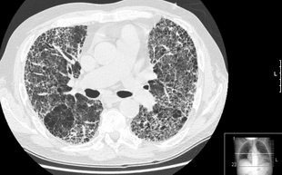\n*Source: Wikipedia*\n\nThis is a prime example of a lung affected with pulmonary fibrosis. Wikipedia describes it as:\n> HRCT of lung showing extensive fibrosis possibly from usual interstitial pneumonitis. There is also a large emphysematous bulla.\n\nTrying to decipher this, I was able to gather that this \"emphysematous bulla\" is always an indicator of pulmonary fibrosis. Here's a more detailed lung with this bulla:\n\n\nSo the bulla is a \"noise\" all over the lungs. However once again, I learnt never to take an assumption for granted by reading through even more:\n\n> Misdiagnosis is common because, while overall pulmonary fibrosis is not rare, each individual type of pulmonary fibrosis is uncommon and the evaluation of patients with these diseases is complex and requires a multidisciplinary approach.\n\nSo with these multiple types of pulmonary fibrosis, it would be difficult to accurately find some underlying factors from the provided data that can easily summarize pulmonary fibrosis from a CT scan. This is the Wikipedia description for the formation of the scar tissue that the scarring causes:\n\n> Pulmonary fibrosis involves gradual exchange of normal lung parenchyma with fibrotic tissue. The replacement of normal lung with scar tissue causes irreversible decrease in oxygen diffusion capacity, and the resulting stiffness or decreased compliance makes pulmonary fibrosis a restrictive lung disease.[13] Pulmonary fibrosis is perpetuated by aberrant wound healing, rather than chronic inflammation.[14] \n\nHere are some key points:\n+ Normal lung becoming scar tissue stifles oxygen diffusion.\n+ It's as effective a disease as it is due to the fact the wound healing is random, and it's aberrant. ","execution_count":null},{"metadata":{"_kg_hide-output":true,"_kg_hide-input":true,"trusted":true,"scrolled":false},"cell_type":"code","source":"!pip install fastai2 -q\n!pip install efficientnet_pytorch -q\n!conda install -c conda-forge gdcm -y\n","execution_count":null,"outputs":[]},{"metadata":{"trusted":true,"scrolled":false},"cell_type":"code","source":"from fastai2.basics import *\nfrom fastai2.medical.imaging import *","execution_count":null,"outputs":[]},{"metadata":{"_uuid":"8f2839f25d086af736a60e9eeb907d3b93b6e0e5","_cell_guid":"b1076dfc-b9ad-4769-8c92-a6c4dae69d19","trusted":true,"_kg_hide-input":true,"scrolled":false},"cell_type":"code","source":"# This Python 3 environment comes with many helpful analytics libraries installed\n# It is defined by the kaggle/python Docker image: https://github.com/kaggle/docker-python\n# For example, here's several helpful packages to load\n\nimport numpy as np # linear algebra\nimport pandas as pd # data processing, CSV file I/O (e.g. pd.read_csv)\nimport pydicom as dcm\nimport os\nimport glob\nimport matplotlib.pyplot as plt\nimport seaborn as sns\np = sns.color_palette()\nimport plotly.offline as py\npy.init_notebook_mode(connected=True)\nimport plotly.graph_objs as go\nimport plotly.tools as tls\nimport cv2","execution_count":null,"outputs":[]},{"metadata":{"_kg_hide-input":true,"trusted":true,"scrolled":false},"cell_type":"code","source":"patient_sizes = [len(os.listdir('../input/osic-pulmonary-fibrosis-progression/train/' + d)) for d in os.listdir('../input/osic-pulmonary-fibrosis-progression/train/')]\nplt.hist(patient_sizes, color=p[2])\nplt.ylabel('Number of patients')\nplt.xlabel('DICOM files')\nplt.title('Histogram of DICOM count per patient');","execution_count":null,"outputs":[]},{"metadata":{},"cell_type":"markdown","source":"As we can see here, we have a lot of patients (subdirectories) with <100 counts being the norm for (most) of the patients. We also have a few patients breaching the 200s and making their way to the 400s or 500s. Could there be any underlying factor?","execution_count":null},{"metadata":{"_kg_hide-input":true,"trusted":true,"scrolled":false},"cell_type":"code","source":"df_train = pd.read_csv('../input/osic-pulmonary-fibrosis-progression/train.csv')\ndf_test = pd.read_csv('../input/osic-pulmonary-fibrosis-progression/test.csv')","execution_count":null,"outputs":[]},{"metadata":{},"cell_type":"markdown","source":"# Train files","execution_count":null},{"metadata":{},"cell_type":"markdown","source":"With DICOM files, we can retrieve the information as a numpy array with the DICOM attribute `ds.pixel_array` from the file which is relatively simple to use. We can invert the colors by adding a `-` before it.","execution_count":null},{"metadata":{"trusted":true,"scrolled":false},"cell_type":"code","source":"r = dcm.dcmread('../input/osic-pulmonary-fibrosis-progression/train/ID00007637202177411956430/11.dcm')\nimg = r.pixel_array\nimg[img == -2000] = 0\n\nplt.axis('off')\nplt.imshow(img)\nplt.show()\n\nplt.axis('off')\nplt.imshow(-img) # Invert colors with -\nplt.show()","execution_count":null,"outputs":[]},{"metadata":{},"cell_type":"markdown","source":"What we can do is **visualize** the DICOM files with a simple glob.glob for the train and test set. It is remarkable that we can extract this information from a DICOM.","execution_count":null},{"metadata":{"_kg_hide-input":true,"trusted":true,"scrolled":false},"cell_type":"code","source":"def show_dcm_info(dataset):\n print(\"Filename.........:\", file_path)\n print()\n\n pat_name = dataset.PatientName\n display_name = pat_name.family_name + \", \" + pat_name.given_name\n print(\"Patient's name......:\", display_name)\n print(\"Patient id..........:\", dataset.PatientID)\n print(\"Patient's Sex.......:\", dataset.PatientSex)\n print(\"Modality............:\", dataset.Modality)\n print(\"Body Part Examined..:\", dataset.BodyPartExamined)\n \n if 'PixelData' in dataset:\n rows = int(dataset.Rows)\n cols = int(dataset.Columns)\n print(\"Image size.......: {rows:d} x {cols:d}, {size:d} bytes\".format(\n rows=rows, cols=cols, size=len(dataset.PixelData)))\n if 'PixelSpacing' in dataset:\n print(\"Pixel spacing....:\", dataset.PixelSpacing)\n dataset.PixelSpacing = [1, 1]\n plt.figure(figsize=(10, 10))\n plt.imshow(dataset.pixel_array, cmap=plt.cm.bone)\n plt.show()\nfor file_path in glob.glob('../input/osic-pulmonary-fibrosis-progression/train/*/*.dcm'):\n dataset = dcm.dcmread(file_path)\n show_dcm_info(dataset)\n break # Comment this out to see all","execution_count":null,"outputs":[]},{"metadata":{},"cell_type":"markdown","source":"This lung image looks very similar to the Data Science Bowl 2017 and it also looks like we have quite a bit of metadata coming with each DICOM file. Now let's examine a couple of images at a glance:","execution_count":null},{"metadata":{"_uuid":"d629ff2d2480ee46fbb7e2d37f6b5fab8052498a","_cell_guid":"79c7e3d0-c299-4dcb-8224-4455121ee9b0","trusted":true,"_kg_hide-input":true,"scrolled":false},"cell_type":"code","source":"files = glob.glob('../input/osic-pulmonary-fibrosis-progression/train/*/*.dcm')\ndef dicom_to_image(filename):\n im = dcm.dcmread(filename)\n img = im.pixel_array\n img[img == -2000] = 0\n return img\nf, plots = plt.subplots(4, 5, sharex='col', sharey='row', figsize=(10, 8))\nfor i in range(20):\n plots[i // 5, i % 5].axis('off')\n plots[i // 5, i % 5].imshow(dicom_to_image(files[i]), cmap=plt.cm.bone)","execution_count":null,"outputs":[]},{"metadata":{},"cell_type":"markdown","source":"All the images look fairly uniform - how about taking into account randomness?","execution_count":null},{"metadata":{"trusted":true,"scrolled":false},"cell_type":"code","source":"files = glob.glob('../input/osic-pulmonary-fibrosis-progression/train/*/*.dcm')\ndef dicom_to_image(filename):\n im = dcm.dcmread(filename)\n img = im.pixel_array\n img[img == -2000] = 0\n return img\nf, plots = plt.subplots(4, 5, sharex='col', sharey='row', figsize=(10, 8))\nfor i in range(20):\n plots[i // 5, i % 5].axis('off')\n plots[i // 5, i % 5].imshow(dicom_to_image(np.random.choice(files)), cmap=plt.cm.bone)","execution_count":null,"outputs":[]},{"metadata":{},"cell_type":"markdown","source":"So some images are uniform but others are not.","execution_count":null},{"metadata":{},"cell_type":"markdown","source":"# Train CSV exploration","execution_count":null},{"metadata":{},"cell_type":"markdown","source":"Let's look at the CSV metadata now.","execution_count":null},{"metadata":{"trusted":true,"_kg_hide-input":true,"scrolled":false},"cell_type":"code","source":"import plotly.io as pio\npio.templates.default = \"ggplot2\"\nxcoord = df_train[\"Age\"].value_counts().keys()\ny1 = df_train[\"Age\"].value_counts().values\n\n\nannotationsList = [dict(\n x=xi,\n y=yi,\n text=str(yi),\n xanchor='right',\n yanchor='bottom',\n showarrow=False,\n ) for xi, yi in zip(xcoord, y1)]\n\n\nannotations = annotationsList\ndata=[go.Bar(\n x=list(df_train['Age'].value_counts().keys()), \n y=list(df_train['Age'].value_counts().values)\n\n)]\nlayout=go.Layout(height=800, width=800, title='Distribution of training labels', annotations=annotations)\nfig=dict(data=data, layout=layout)\npy.iplot(fig, filename='train-label-dist')","execution_count":null,"outputs":[]},{"metadata":{},"cell_type":"markdown","source":"How about the duration? HMMMMM....","execution_count":null},{"metadata":{"trusted":true,"scrolled":false},"cell_type":"code","source":"import plotly.express as px\ndata=px.bar(x=list(df_train['Weeks'].value_counts().keys()), y=list(df_train['Weeks'].value_counts().values))\ndata","execution_count":null,"outputs":[]},{"metadata":{},"cell_type":"markdown","source":"So it seems like we have a rather lackadaisical distribution of Age in the data which is interesting to consider. How about the target distribution in the data? (FVC)","execution_count":null},{"metadata":{"trusted":true,"scrolled":false},"cell_type":"code","source":"plt.style.use('seaborn-darkgrid')\ndata=plt.scatter(x=list(df_train['FVC'].value_counts().keys()), y=list(df_train['FVC'].value_counts().values))\ndata;","execution_count":null,"outputs":[]},{"metadata":{},"cell_type":"markdown","source":"So as of now, let's take a look at smoking status of each affected person (i.e whether the person is a former smoker, whether the person never smoked, or whether the person currently smokes) for perspective.","execution_count":null},{"metadata":{"_kg_hide-input":true,"trusted":true,"scrolled":false},"cell_type":"code","source":"cnts = df_train['SmokingStatus'].value_counts()\ncnts = cnts/cnts.sum() # convert to percentage\n\n\n# Plot\n# Set order and colors\nsns.set()\npref_order = ['Ex-smoker', 'Never smoked', 'Currently smokes']\npref_color = ['#F7819F', '#F5A9BC', '#E6E6E6']\n\n# matplotlib general settings\nfig, ax = plt.subplots(figsize=(20,1))\nplt.title('Smoking Status', fontsize=18, loc='left')\nax.get_xaxis().set_visible(False)\nax.tick_params(axis='y', labelsize=16, labelcolor='grey') \nax.set_facecolor('white')\n\n# Draw each bar and text separately with appropriate offset\nbar_start = 0\nfor i in pref_order:\n ax.barh(y=[3], width=cnts[i], height=0.1, left=bar_start, color=pref_color[pref_order.index(i)])\n #plt.text(bar_start + (cnts[i])/2 - 0.015, 0.4, \"{:.0%}\".format(cnts[i]), fontsize=16, transform=ax.transAxes)\n bar_start += cnts[i]\n\n# Draw legend and set color of its text\nleg = ax.legend(pref_order, loc=(0.18,-0.5), ncol=5, fontsize=14, frameon=True, facecolor='white');\nfor txt in leg.get_texts():\n plt.setp(txt, color='grey')","execution_count":null,"outputs":[]},{"metadata":{},"cell_type":"markdown","source":"The majority of people here are ex-smokers (approximately a third of people) and as such, we can explore further based on gender (i.e. percentage of each per male and female).","execution_count":null},{"metadata":{"_kg_hide-input":true,"trusted":true,"scrolled":false},"cell_type":"code","source":"categories = ['Male', 'Female']\n\n# Empty df to be built out\ncnts = pd.DataFrame(columns = categories)\n\n# Loop over all age categories and get distribution of responses \nfor cat in categories:\n cnts[cat] = df_train.loc[df_train['Sex'] == cat, 'SmokingStatus'].value_counts()\n\n# Drop those with no opinion\ncnts = cnts/cnts.sum() # convert to percentage\n\n\n# Plot\n\n# matplotlib settings\nfig, ax = plt.subplots(figsize=(20,3))\nplt.title('Smoking status per gender', fontsize=18, loc='left')\nax.get_xaxis().set_visible(False)\nax.tick_params(axis='y', labelsize=16, labelcolor='grey') \nax.set_facecolor('white')\n\n# Draw each bar and text separately with appropriate offset\nfor cat in categories:\n bar_start = 0\n for i in pref_order:\n ax.barh(y=[cat], width=cnts.loc[i,cat], height=0.6, left=bar_start, color=pref_color[pref_order.index(i)])\n bar_start += cnts.loc[i,cat]\n\n# Draw legend and set color of its text\nleg = ax.legend(pref_order, loc=(0.18,-0.2), ncol=5, fontsize=14, frameon=True, facecolor='white');\nfor txt in leg.get_texts():\n plt.setp(txt, color='grey')","execution_count":null,"outputs":[]},{"metadata":{},"cell_type":"markdown","source":"There's a huge difference between male and female over here in that the majority of males affected are former smokers and the majority of females affected have never smoked.","execution_count":null},{"metadata":{},"cell_type":"markdown","source":"# Fast.ai! (yay :3)","execution_count":null},{"metadata":{},"cell_type":"markdown","source":"Now with Fast.ai, it becomes a lot easier for us to try and handle the data. We can work with something called \"systematic windowing\" which was previously used by radiologists with regards to the brain (see the excellent notebook by Jemery Howard here: https://www.kaggle.com/jhoward/don-t-see-like-a-radiologist-fastai ) and we can easily view the details of the lungs with systematic windowing.","execution_count":null},{"metadata":{"trusted":true,"scrolled":false},"cell_type":"code","source":"fn = Path('../input/osic-pulmonary-fibrosis-progression/train/ID00026637202179561894768')\nfname = Path('../input/osic-pulmonary-fibrosis-progression/train/ID00007637202177411956430/13.dcm')\ndcom = fname.dcmread()\ndcom.show(scale=dicom_windows.lungs)","execution_count":null,"outputs":[]},{"metadata":{},"cell_type":"markdown","source":"Well, windowing works particularly well for computers (because us humans require a lot more than simple black, white and grey) so we can try some sort of \"better\" windowing in a rainbow colormap. The background ought to be black instead of a weird psychedelic *Neon Genesis Evangelion* style but it works well. A warning is due: it is shockingly bright.","execution_count":null},{"metadata":{"trusted":true,"scrolled":false},"cell_type":"code","source":"dcom.show(cmap='turbo', figsize=(6,6))","execution_count":null,"outputs":[]},{"metadata":{},"cell_type":"markdown","source":"The turbo colormap which I have copy-pasted at the top of this notebook is shockingly bright, but it exposes the amount of empty space that we have in the image.","execution_count":null},{"metadata":{"trusted":true,"scrolled":false},"cell_type":"code","source":"mask = dcom.mask_from_blur(dicom_windows.lungs)\nwind = dcom.windowed(*dicom_windows.lungs)\n\n_,ax = subplots(1,1)\nshow_image(wind, ax=ax[0])\nshow_image(mask, alpha=0.5, cmap=plt.cm.Reds, ax=ax[0]);","execution_count":null,"outputs":[]},{"metadata":{},"cell_type":"markdown","source":"Here we can see the distinctions.","execution_count":null},{"metadata":{"trusted":true,"scrolled":false},"cell_type":"code","source":"bbs = mask2bbox(mask)\nlo,hi = bbs\nshow_image(wind[lo[0]:hi[0],lo[1]:hi[1]]);","execution_count":null,"outputs":[]},{"metadata":{},"cell_type":"markdown","source":"Now we can isolate the lungs from the empty space.","execution_count":null},{"metadata":{},"cell_type":"markdown","source":"Now that you have got over your eyes going kaboom, let us proceed to a more, shall I say, medical, view of things with the courtesy of fast.ai and Jeremy Howard.","execution_count":null},{"metadata":{"trusted":true,"scrolled":false},"cell_type":"code","source":"path = Path('../input/osic-pulmonary-fibrosis-progression/train/ID00007637202177411956430/')\ndef fix_pxrepr(dcm):\n if dcm.PixelRepresentation != 0 or dcm.RescaleIntercept<-100: return\n x = dcm.pixel_array + 1000\n px_mode = 4096\n x[x>=px_mode] = x[x>=px_mode] - px_mode\n dcm.PixelData = x.tobytes()\n dcm.RescaleIntercept = -1000","execution_count":null,"outputs":[]},{"metadata":{},"cell_type":"markdown","source":"The above basically just fixes up the pixel representation attribute of the DICOM file for us to use.","execution_count":null},{"metadata":{"trusted":true,"scrolled":false},"cell_type":"code","source":"def dcm_tfm(fn): \n fn = (path/fn).with_suffix('.dcm')\n try:\n x = fn.dcmread()\n fix_pxrepr(x)\n except Exception as e:\n pass\n if x.Rows != 512 or x.Columns != 512: x.zoom_to((512,512))\n px = x.scaled_px\n return TensorImage(px.to_3chan(dicom_windows.lungs,dicom_windows.subdural, bins=None))","execution_count":null,"outputs":[]},{"metadata":{},"cell_type":"markdown","source":"This basically reads in a DICOM file, fixes up its pixel representation attribute (as I have displayed earlier with the previous one) and it then returns a Tensor image. It fixes up our files for a neat data loader in case we ever want to use it in our modeling pipelines. This also belongs to Jeremy Howard: https://www.kaggle.com/jhoward/cleaning-the-data-for-rapid-prototyping-fastai ).","execution_count":null},{"metadata":{"trusted":true,"scrolled":false},"cell_type":"code","source":"show_images(dcm_tfm('1'))","execution_count":null,"outputs":[]},{"metadata":{},"cell_type":"markdown","source":"The above is basically just our earlier image in Tensor format for a neural network to utilize.","execution_count":null},{"metadata":{"trusted":true,"scrolled":false},"cell_type":"code","source":"px = dcom.windowed(*dicom_windows.lungs)\nshow_image(px);","execution_count":null,"outputs":[]},{"metadata":{},"cell_type":"markdown","source":"This crops out the above neatly to leave just the lungs remaining right where we want them. However, we must be careful with loss of information as not even a robot would be willing to waste its valuable time examining miniscule patches on digital DICOM images.","execution_count":null},{"metadata":{"trusted":true,"scrolled":false},"cell_type":"code","source":"_,axs = subplots(1,2)\ndcom.show(ax=axs[0]); dcom.show(dicom_windows.lungs, ax=axs[1])","execution_count":null,"outputs":[]},{"metadata":{},"cell_type":"markdown","source":"This function however, has a rather unique purpose which is to display our DICOM files but with a twist: it first displays the normal image and then it displays our windowed image (scroll up to check what is windowing or go to the RSNA comp and look at a couple of notebooks). We can try a gaussian blur to smooth out the bad parts here.","execution_count":null},{"metadata":{"trusted":true,"scrolled":false},"cell_type":"code","source":"gdcm = gauss_blur2d(dcom.windowed(*dicom_windows.brain), 100) # using the brain for visualization purposes\nshow_image(gdcm);","execution_count":null,"outputs":[]},{"metadata":{},"cell_type":"markdown","source":"..and now to shamelessly use an idea from Jeremy (again) and select the areas bright enough in the picture (segment it)","execution_count":null},{"metadata":{"trusted":true,"scrolled":false},"cell_type":"code","source":"show_image(gdcm>0.3);","execution_count":null,"outputs":[]},{"metadata":{},"cell_type":"markdown","source":"Now create a simple mask for our image which (albeit looks weird without the main image) will serve certain purposes for us when it comes to modeling.","execution_count":null},{"metadata":{"_kg_hide-input":true,"trusted":true,"scrolled":false},"cell_type":"code","source":"show_image(dcom.mask_from_blur(dicom_windows.lungs), cmap=plt.cm.Reds, alpha=0.6);","execution_count":null,"outputs":[]},{"metadata":{},"cell_type":"markdown","source":"All this does is reduce the image to a smaller one *without* the unnecessary area at the bottom of the image.","execution_count":null},{"metadata":{"_kg_hide-input":true,"trusted":true,"scrolled":false},"cell_type":"code","source":"def pad_square(x):\n r,c = x.shape\n d = (c-r)/2\n pl,pr,pt,pb = 0,0,0,0\n if d>0: pt,pd = int(math.floor( d)),int(math.ceil( d)) \n else: pl,pr = int(math.floor(-d)),int(math.ceil(-d))\n return np.pad(x, ((pt,pb),(pl,pr)), 'minimum')\n\ndef crop_mask(x):\n mask = x.mask_from_blur(dicom_windows.lungs)\n bb = mask2bbox(mask)\n if bb is None: return\n lo,hi = bb\n cropped = x.pixel_array[lo[0]:hi[0],lo[1]:hi[1]]\n x.pixel_array = pad_square(cropped)\n_,axs = subplots(1,2)\ndcom.show(ax=axs[0])\ncrop_mask(dcom)\ndcom.show(ax=axs[1]);","execution_count":null,"outputs":[]},{"metadata":{},"cell_type":"markdown","source":"As we have seen, it is possible to toy with DICOM files. However, now we can convert a DICOM to a data frmae.","execution_count":null},{"metadata":{"trusted":true,"scrolled":false},"cell_type":"code","source":"df = pd.DataFrame.from_dicoms(fn.ls())\ndf.head()","execution_count":null,"outputs":[]},{"metadata":{},"cell_type":"markdown","source":"And toy with the data (again)","execution_count":null},{"metadata":{"trusted":true,"_kg_hide-input":true,"scrolled":false},"cell_type":"code","source":"import plotly.express as px\nselected_data = df\nN = len(df.img_mean)\ntrace1 = go.Scatter3d(\n x=selected_data.img_mean.values[0:N], \n y=selected_data.img_std.values[0:N],\n z=selected_data.img_pct_window.values[0:N],\n mode='markers',\n marker=dict(\n colorscale = \"Jet\",\n colorbar=dict(thickness=10, title=\"image columns\", len=0.8),\n opacity=0.4,\n size=2\n )\n)\n\nfigure_data = [trace1]\nlayout = go.Layout(\n title = \"Visualizing Mean, Stddev and Window values\",\n scene = dict(\n xaxis = dict(title=\"Image mean\"),\n yaxis = dict(title=\"Image standard deviation\"),\n zaxis = dict(title=\"Image window values\"),\n ),\n margin=dict(\n l=0,\n r=0,\n b=0,\n t=0\n ),\n showlegend=True\n)\n\nfig = go.Figure(data=figure_data, layout=layout)\npy.iplot(fig, filename='simple-3d-scatter')","execution_count":null,"outputs":[]},{"metadata":{},"cell_type":"markdown","source":"Now that it is possible for us to visualize the distribution, it's actually possible for us to view it as a correlation matrix with Plot.ly of course (I am bored of Seaborn :p).","execution_count":null},{"metadata":{},"cell_type":"markdown","source":"Now we can view the distributions of image statistics one-by-one:","execution_count":null},{"metadata":{"trusted":true},"cell_type":"code","source":"def distrib_summ(t):\n plt.hist(t,40)\n return array([t.min(),*np.percentile(t,[0.1,1,5,50,95,99,99.9]),t.max()], dtype=np.int)\ndistrib_summ(df.img_max.values)","execution_count":null,"outputs":[]},{"metadata":{},"cell_type":"markdown","source":"Not such a comfortable distribution to be working with....","execution_count":null},{"metadata":{"trusted":true},"cell_type":"code","source":"distrib_summ(df.img_std.values)","execution_count":null,"outputs":[]},{"metadata":{},"cell_type":"markdown","source":"Rather odd distribution over here too.","execution_count":null},{"metadata":{"trusted":true},"cell_type":"code","source":"distrib_summ(df.img_pct_window.values)","execution_count":null,"outputs":[]},{"metadata":{},"cell_type":"markdown","source":"Now to move on to preprocessing.","execution_count":null},{"metadata":{},"cell_type":"markdown","source":"# Preprocessing (credits to Guido Zuidhof)","execution_count":null},{"metadata":{},"cell_type":"markdown","source":"The functions and 3d plotting are from Guido's notebook: https://www.kaggle.com/gzuidhof/full-preprocessing-tutorial and I've tried to add clarity wherevr possible to whatever Guido has done here.","execution_count":null},{"metadata":{"trusted":true,"scrolled":false},"cell_type":"code","source":"import os\nimport pydicom as dicom, numpy as np\nfrom matplotlib import pyplot as plt\ndef load_scan(path):\n slices = [dicom.read_file(path + '/' + s) for s in os.listdir(path)]\n slices.sort(key = lambda x: float(x.ImagePositionPatient[2]))\n try:\n slice_thickness = np.abs(slices[0].ImagePositionPatient[2] - slices[1].ImagePositionPatient[2])\n except:\n slice_thickness = np.abs(slices[0].SliceLocation - slices[1].SliceLocation)\n \n for s in slices:\n s.SliceThickness = slice_thickness\n \n return slices","execution_count":null,"outputs":[]},{"metadata":{},"cell_type":"markdown","source":"So what this does is basically get the dicom files, sort the files and get slice thickness and make it a file property (or modify the SliceThickness attribute if the attribute exists).","execution_count":null},{"metadata":{"trusted":true,"scrolled":false},"cell_type":"code","source":"def get_pixels_hu(slices):\n image = np.stack([s.pixel_array for s in slices])\n # Convert to int16 (from sometimes int16), \n # should be possible as values should always be low enough (<32k)\n image = image.astype(np.int16)\n\n # Set outside-of-scan pixels to 0\n # The intercept is usually -1024, so air is approximately 0\n image[image == -2000] = 0\n \n # Convert to Hounsfield units (HU)\n for slice_number in range(len(slices)):\n \n intercept = slices[slice_number].RescaleIntercept\n slope = slices[slice_number].RescaleSlope\n \n if slope != 1:\n image[slice_number] = slope * image[slice_number].astype(np.float64)\n image[slice_number] = image[slice_number].astype(np.int16)\n \n image[slice_number] += np.int16(intercept)\n \n return np.array(image, dtype=np.int16)","execution_count":null,"outputs":[]},{"metadata":{},"cell_type":"markdown","source":"This gets the Hounsfield Units (a measurement to which the CT scanners are delicately calibrated to) and Guido calls it:\n> a measure of radiodensity\n\nSo for those of you unenlightened on the subject of radiodensity, I looked it up quickly, and to quote Wikipedia:\n> Radiodensity (or radiopacity) is opacity to the radio wave and X-ray portion of the electromagnetic spectrum: that is, the relative inability of those kinds of electromagnetic radiation to pass through a particular material.\n\nIn layman's terms, it's the ability of a certain kind of material to prevent radio waves or X-rays to pass through them.","execution_count":null},{"metadata":{"trusted":true,"scrolled":false},"cell_type":"code","source":"first_patient = load_scan('../input/osic-pulmonary-fibrosis-progression/train/ID00007637202177411956430/')\nfirst_patient_pixels = get_pixels_hu(first_patient)\nfig, ax = plt.subplots()\nplt.hist(first_patient_pixels.flatten(), bins=80, color='c')\nplt.xlabel(\"Hounsfield Units (HU)\")\nplt.ylabel(\"Frequency\")\n\nplt.show()","execution_count":null,"outputs":[]},{"metadata":{},"cell_type":"markdown","source":"We also can visualize convolution filters:","execution_count":null},{"metadata":{"trusted":true,"scrolled":false},"cell_type":"code","source":"import cv2\nimg = dicom.dcmread('../input/osic-pulmonary-fibrosis-progression/test/ID00419637202311204720264/1.dcm')\ndef conv(img):\n fig, ax = plt.subplots(nrows=1, ncols=2, figsize=(20, 20))\n kernel = np.ones((7, 7), np.float32)/25\n conv = cv2.filter2D(img, -1, kernel)\n ax[0].imshow(img)\n ax[0].set_title('Original Image', fontsize=24)\n ax[1].imshow(conv)\n ax[1].set_title('Convolved Image', fontsize=24)\n plt.show()\nconv(img.pixel_array)","execution_count":null,"outputs":[]},{"metadata":{},"cell_type":"markdown","source":"This is now our fully preprocessed image, in full 3d glory.","execution_count":null},{"metadata":{"trusted":true},"cell_type":"code","source":"from skimage import measure, morphology\nfrom mpl_toolkits.mplot3d.art3d import Poly3DCollection\ndef plot_3d(image, threshold=700):\n \n # Position the scan upright, \n # so the head of the patient would be at the top facing the camera\n p = image.transpose(2,1,0)\n \n verts, faces,_,_ = measure.marching_cubes_lewiner(p, threshold)\n\n fig = plt.figure(figsize=(10, 10))\n ax = fig.add_subplot(111, projection='3d')\n\n # Fancy indexing: `verts[faces]` to generate a collection of triangles\n mesh = Poly3DCollection(verts[faces])\n mesh.set_edgecolor('b')\n ax.add_collection3d(mesh)\n\n ax.set_xlim(0, p.shape[0])\n ax.set_ylim(0, p.shape[1])\n ax.set_zlim(0, p.shape[2])\n\n plt.show()\nplot_3d(first_patient_pixels)","execution_count":null,"outputs":[]},{"metadata":{},"cell_type":"markdown","source":"Beautiful! Now we can attempt to segment the lungs. This thresholds the image, adds the connected components, and within the filled segmented lungs attempts to create some bronchiole-like structure.","execution_count":null},{"metadata":{"_kg_hide-input":true,"trusted":true},"cell_type":"code","source":"def largest_label_volume(im, bg=-1):\n vals, counts = np.unique(im, return_counts=True)\n\n counts = counts[vals != bg]\n vals = vals[vals != bg]\n\n if len(counts) > 0:\n return vals[np.argmax(counts)]\n else:\n return None\n\ndef segment_lung_mask(image, fill_lung_structures=True):\n \n # not actually binary, but 1 and 2. \n # 0 is treated as background, which we do not want\n binary_image = np.array(image > -320, dtype=np.int8)+1\n labels = measure.label(binary_image)\n \n # Pick the pixel in the very corner to determine which label is air.\n # Improvement: Pick multiple background labels from around the patient\n # More resistant to \"trays\" on which the patient lays cutting the air \n # around the person in half\n background_label = labels[0,0,0]\n \n #Fill the air around the person\n binary_image[background_label == labels] = 2\n \n \n # Method of filling the lung structures (that is superior to something like \n # morphological closing)\n if fill_lung_structures:\n # For every slice we determine the largest solid structure\n for i, axial_slice in enumerate(binary_image):\n axial_slice = axial_slice - 1\n labeling = measure.label(axial_slice)\n l_max = largest_label_volume(labeling, bg=0)\n \n if l_max is not None: #This slice contains some lung\n binary_image[i][labeling != l_max] = 1\n\n \n binary_image -= 1 #Make the image actual binary\n binary_image = 1-binary_image # Invert it, lungs are now 1\n \n # Remove other air pockets insided body\n labels = measure.label(binary_image, background=0)\n l_max = largest_label_volume(labels, bg=0)\n if l_max is not None: # There are air pockets\n binary_image[labels != l_max] = 0\n \n return binary_image\nsegmented_lungs = segment_lung_mask(first_patient_pixels, False)\nsegmented_lungs_fill = segment_lung_mask(first_patient_pixels, True)\nplot_3d(segmented_lungs, 0)","execution_count":null,"outputs":[]},{"metadata":{},"cell_type":"markdown","source":"This is a very naive form of preprocessing, as it primarily only segments a part of the lungs and leaves the rest up for grabs. However, checking the filling in the lungs could perhaps serve us better...","execution_count":null},{"metadata":{"trusted":true},"cell_type":"code","source":"plot_3d(segmented_lungs_fill, 0)","execution_count":null,"outputs":[]},{"metadata":{},"cell_type":"markdown","source":"Let's check the difference to see whether this method is actually feasible.","execution_count":null},{"metadata":{"trusted":true},"cell_type":"code","source":"plot_3d(segmented_lungs_fill - segmented_lungs, 0)","execution_count":null,"outputs":[]},{"metadata":{},"cell_type":"markdown","source":"It seems like this method is a dead end for now....","execution_count":null},{"metadata":{},"cell_type":"markdown","source":"# Afterword: a better preprocessing?\n\nSo yes, we do need to preprocess a load of images, considering the discrepancies between most of our train images, especially with regards to the border (which is either circular or nonexistent in most cases). We might need to even this out, so in that case I'll be taking the aid of Roman's microscope augmentation (again another idea from SIIM-ISIC competition) over here: https://www.kaggle.com/c/siim-isic-melanoma-classification/discussion/159476 .\n\nAs you can see in the following image from the notebook [Your Starter Notebook for OSIC!](https://www.kaggle.com/twinkle0705/your-starter-notebook-for-osic) we have the circular/nonexistent border discrepancy. So again, we can treat this with Roman's microscope augmentation, as in the SIIM-ISIC competition the same thing existed.","execution_count":null},{"metadata":{"trusted":true,"scrolled":false},"cell_type":"code","source":"import random\nclass Microscope:\n def __init__(self, p: float = 0.5):\n self.p = p\n\n def __call__(self, img):\n if random.random() < self.p:\n circle = cv2.circle((np.ones(img.shape) * 255).astype(np.uint8),\n (img.shape[0]//2, img.shape[1]//2),\n random.randint(img.shape[0]//2 - 3, img.shape[0]//2 + 15),\n (0, 0, 0),\n -1)\n\n mask = circle - 255\n img = np.multiply(img, mask)\n\n return img\n \nimport pydicom\ndcom_file = pydicom.dcmread('../input/osic-pulmonary-fibrosis-progression/train/ID00009637202177434476278/100.dcm')\nfig, ax = plt.subplots(1, 2, figsize=(10, 10))\nax[0].set_title('Before the Aug')\nax[0].imshow(dcom_file.pixel_array, cmap='turbo')\nax[1].set_title('After the Aug')\nmicro = Microscope(p=0.5)\nax[1].imshow(micro(dcom_file.pixel_array), cmap='turbo')\nax[0].axis('off')\nax[1].axis('off')","execution_count":null,"outputs":[]},{"metadata":{},"cell_type":"markdown","source":"Now, however, we have normalized the images and found a pretty good colormap to use. So that takes care of our first problem. The second problem however is to see how we can improve on Roman's work. Now we can turn to the methods of Neuron Engineer, whose preprocessing methods have been enumerated on many times previously by other notebooks, including mine on SIIM-ISIC. \n\nHe's using Ben Graham's technique (which won a first place in the diabetic retinopathy competition) and if you want to look deeper in the preprocessing methods, refer to the following link: https://www.kaggle.com/ratthachat/aptos-eye-preprocessing-in-diabetic-retinopathy\n\nNow here we can use both Ben Graham's and Roman's techniques in conjunction with each other, by performing the microscope augmentation technique and then adding a gaussian blur from Ben's work. Normally, adding a Gaussian blur would be much more difficult - if not for fast.ai and the magic of its medical imaging module.","execution_count":null},{"metadata":{"_kg_hide-input":true,"trusted":true,"scrolled":false},"cell_type":"code","source":"import tempfile\nimport datetime\n\nimport pydicom\nfrom pydicom.dataset import Dataset, FileDataset, FileMetaDataset\n\n# Create some temporary filenames\nsuffix = '.dcm'\nfilename_little_endian = tempfile.NamedTemporaryFile(suffix=suffix).name\nfilename_big_endian = tempfile.NamedTemporaryFile(suffix=suffix).name\n\nprint(\"Setting file meta information...\")\n# Populate required values for file meta information\nfile_meta = FileMetaDataset()\nfile_meta.MediaStorageSOPClassUID = '1.2.840.10008.5.1.4.1.1.2'\nfile_meta.MediaStorageSOPInstanceUID = \"1.2.3\"\nfile_meta.ImplementationClassUID = \"1.2.3.4\"\n\nprint(\"Setting dataset values...\")\n# Create the FileDataset instance (initially no data elements, but file_meta\n# supplied)\nds = FileDataset(filename_little_endian, {},\n file_meta=file_meta, preamble=b\"\\0\" * 128)\n\n# Add the data elements -- not trying to set all required here. Check DICOM\n# standard\nds.PatientName = \"Test^Firstname\"\nds.PatientID = \"123456\"\n\n# Set the transfer syntax\nds.is_little_endian = True\nds.is_implicit_VR = True\n\n# Set creation date/time\ndt = datetime.datetime.now()\nds.ContentDate = dt.strftime('%Y%m%d')\ntimeStr = dt.strftime('%H%M%S.%f') # long format with micro seconds\nds.ContentTime = timeStr\n\nprint(\"Writing test file\", filename_little_endian)\nds.save_as(filename_little_endian)\nprint(\"File saved.\")\nds.PhotometricInterpretation = 'MONOCHROME2'\nds.PixelRepresentation = 0\nds.SamplesPerPixel = 1\n# Write as a different transfer syntax XXX shouldn't need this but pydicom\n# 0.9.5 bug not recognizing transfer syntax\nds.file_meta.TransferSyntaxUID = pydicom.uid.ExplicitVRBigEndian\nds.is_little_endian = False\nds.is_implicit_VR = False\nds.pixel_array = micro(dcom_file.pixel_array)\nds.BitsAllocated = len(micro(dcom_file.pixel_array))\nprint(\"Writing test file as Big Endian Explicit VR\", filename_big_endian)\nds.save_as(filename_big_endian)\nfn = Path('../input/osic-pulmonary-fibrosis-progression/train/ID00007637202177411956430/')\nfname = Path(filename_big_endian)\ndcom = fname.dcmread()\ndcom.file_meta.TransferSyntaxUID = pydicom.uid.ExplicitVRBigEndian\ndcom.pixel_array = micro(dcom_file.pixel_array)\ndcom.BitsAllocated = 16\ndcom.PhotometricInterpretation = 'MONOCHROME2'\ndcom.PixelRepresentation = 0\ndcom.SamplesPerPixel = 1\ndcom.Modality = 'CT'\ndcom.RescaleSlope = \"1.0\"\ndcom.RescaleIntercept = \"-1024.0\"\ngdcm = gauss_blur2d(dcom.windowed(*dicom_windows.brain), 14) # using the brain for visualization purposes\nfig, ax = plt.subplots(1, 2, figsize=(10, 10))\nax[0].set_title('Before the Aug')\nax[0].imshow(dcom_file.pixel_array, cmap='turbo')\nax[1].set_title('After the Aug')\nmicro = Microscope(p=0.5)\nax[1].imshow(gdcm, cmap='turbo')\nax[0].axis('off')\nax[1].axis('off')","execution_count":null,"outputs":[]},{"metadata":{},"cell_type":"markdown","source":"So this is the complete merger of both Roman's and Ben's augmentations, you can use this \"slightly\" blurred image for your modeling purposes, and since it's been microscoped it would work pretty nicely.","execution_count":null},{"metadata":{"_kg_hide-input":true,"trusted":true,"scrolled":false},"cell_type":"code","source":"import gc;gc.collect()","execution_count":null,"outputs":[]},{"metadata":{},"cell_type":"markdown","source":"## Proposed aug: Roman's hair augs","execution_count":null},{"metadata":{"trusted":true},"cell_type":"code","source":"class AdvancedHairAugmentation:\n def __init__(self, hairs: int = 4, hairs_folder: str = \"\"):\n self.hairs = hairs\n self.hairs_folder = hairs_folder\n\n def __call__(self, img):\n n_hairs = random.randint(0, self.hairs)\n\n if not n_hairs:\n return img\n\n height, width, _ = img.shape # target image width and height\n hair_images = [im for im in os.listdir(self.hairs_folder) if 'png' in im]\n\n for _ in range(n_hairs):\n hair = cv2.imread(os.path.join(self.hairs_folder, random.choice(hair_images)))\n hair = cv2.flip(hair, random.choice([-1, 0, 1]))\n hair = cv2.rotate(hair, random.choice([0, 1, 2]))\n \n h_height, h_width, _ = hair.shape # hair image width and height\n roi_ho = random.randint(0, img.shape[0] - hair.shape[0])\n roi_wo = random.randint(0, img.shape[1] - hair.shape[1])\n roi = img[roi_ho:roi_ho + h_height, roi_wo:roi_wo + h_width]\n\n img2gray = cv2.cvtColor(hair, cv2.COLOR_BGR2GRAY)\n ret, mask = cv2.threshold(img2gray, 10, 255, cv2.THRESH_BINARY)\n mask_inv = cv2.bitwise_not(mask)\n img_bg = cv2.bitwise_and(roi, roi, mask=mask_inv)\n hair_fg = cv2.bitwise_and(hair, hair, mask=mask)\n\n dst = cv2.add(img_bg, hair_fg)\n img[roi_ho:roi_ho + h_height, roi_wo:roi_wo + h_width] = dst\n\n return img","execution_count":null,"outputs":[]},{"metadata":{},"cell_type":"markdown","source":"# Building a baseline model\n\n","execution_count":null},{"metadata":{},"cell_type":"markdown","source":"Here are some objectives of our *baseline* model that we will add to it:\n+ **Some basic transforms**: We can use some simple `torchvision` transforms w/ our model, such as ToTensor and torchvision normalization. This will help our model to potentially generalize well, what with the diversity we're adding to our trianing data and what not.\n+ **Simple CNN-based model**: This will be using a simple convolutional neural network-based model w/ the assistance of PyTorch, and I will also attempt clumsily to demonstrate each layer in detail using the torchsummary package.","execution_count":null},{"metadata":{"_kg_hide-input":true,"trusted":true,"scrolled":false},"cell_type":"code","source":"import torch\nimport torch.nn as nn\nimport torch.nn.functional as F\nfrom pathlib import Path","execution_count":null,"outputs":[]},{"metadata":{},"cell_type":"markdown","source":"I initially wanted to use [Carlos Souza's excellent End-to-end model notebook's data generator](https://www.kaggle.com/carlossouza/end-to-end-model-ct-scans-tabular) for the data preprocessing and generation part. However, I decided to use his preprocessed CT Scans in conjunction with his data loader for demo purposes.","execution_count":null},{"metadata":{"_kg_hide-input":true,"trusted":true,"scrolled":false},"cell_type":"code","source":"class CTTensorsDataset(torch.utils.data.Dataset):\n def __init__(self, root_dir, transform=None):\n self.root_dir = Path(root_dir)\n self.tensor_files = sorted([f for f in self.root_dir.glob('*.pt')])\n self.transform = transform\n\n def __len__(self):\n return len(self.tensor_files)\n\n def __getitem__(self, item):\n if torch.is_tensor(item):\n item = item.tolist()\n\n image = torch.load(self.tensor_files[item])\n if self.transform:\n image = self.transform(image)\n\n return {\n 'patient_id': self.tensor_files[item].stem,\n 'image': image\n }\n\n def mean(self):\n cum = 0\n for i in range(len(self)):\n sample = self[i]['image']\n cum += torch.mean(sample).item()\n\n return cum / len(self)\n\n def random_split(self, val_size: float):\n num_val = int(val_size * len(self))\n num_train = len(self) - num_val\n return random_split(self, [num_train, num_val])\n \ntrain = CTTensorsDataset(\n root_dir=Path('../input/osic-cached-dataset')\n)\ncum = 0\nfor i in range(len(train)):\n sample = train[i]['image']\n cum += torch.mean(sample).item()","execution_count":null,"outputs":[]},{"metadata":{},"cell_type":"markdown","source":"Now here are the transforms: random sized crop, random flipping, convert to tensor and normalization.","execution_count":null},{"metadata":{"trusted":true,"scrolled":false},"cell_type":"code","source":"dataloader = torch.utils.data.DataLoader(train, batch_size=4,\n shuffle=True, num_workers=4)","execution_count":null,"outputs":[]},{"metadata":{},"cell_type":"markdown","source":"Now we're going to define a Model class so that we're able to train this CNN based model on our input images.","execution_count":null},{"metadata":{"trusted":true,"scrolled":false},"cell_type":"code","source":"class depthwise_separable_conv(nn.Module):\n def __init__(self, nin, kernels_per_layer, nout):\n super(depthwise_separable_conv, self).__init__()\n self.depthwise = nn.Conv2d(nin, nin * kernels_per_layer, kernel_size=3, padding=1)\n self.pointwise = nn.Conv2d(nin * kernels_per_layer, nout, kernel_size=1)\n \n def forward(self, x):\n out = self.depthwise(x)\n out = self.pointwise(out)\n return out\n \nclass Model(nn.Module):\n def __init__(self):\n super(Model, self).__init__()\n self.dsconv1 = nn.Conv3d(1, 16, 3)\n self.dsconv2 = nn.Conv3d(16, 32, 3)\n self.d = nn.Dropout(p=0.2)\n self.m = nn.MaxPool3d((3, 3, 2), stride=(2, 2, 1))\n \n def forward(self, inputs):\n x = self.dsconv1(inputs)\n x = self.dsconv2(x)\n x = self.m(x)\n x = self.d(x)\n x = torch.flatten(x, 1)\n return x","execution_count":null,"outputs":[]},{"metadata":{},"cell_type":"markdown","source":"#### Explanation of model architecture\n\nFirst of all, I already said that depthwise-pointwise convolutions will be the main event in our model, so as such, allow me to present to you the formula for a simple convolution:\n\n$$out(N_i, C_{out_j}) = bias(C_{out_j}) +\n \\sum_{k = 0}^{C_{in} - 1} weight(C_{out_j}, k) \\star input(N_i, k)$$\n\nNow a depthwise convolution takes the `groups` parameter (and it declares the output shape as the input shape multiplied by kernels per layer) and defines it as the same as the input shape. The pointwise convolution does away wit the groups and then processes the depthwise convolution to return an output. \n\nDepthwise convolutions would be better suited for TensorFlow rather than PyTorch because of the way they are optimized in PyTorch rather than TF, however I'm solely writing this in PyTorch for learning purposes.","execution_count":null},{"metadata":{},"cell_type":"markdown","source":"# Metric learning","execution_count":null},{"metadata":{"trusted":true},"cell_type":"code","source":"class MetricOptimizer:\n \n def __init__(self, raw, labs, conf):\n self.raw = raw\n self.conf = conf\n self.labs = labs\n \n def lllloss(self, actual_fvc, predicted_fvc, confidence, return_values = False):\n \"\"\"\n Calculates the modified Laplace Log Likelihood score for this competition.\n \"\"\"\n sd_clipped = np.maximum(confidence, 70)\n delta = np.minimum(np.abs(actual_fvc - predicted_fvc), 1000)\n metric = - np.sqrt(2) * delta / sd_clipped - np.log(np.sqrt(2) * sd_clipped)\n\n if return_values:\n return metric\n else:\n return np.mean(metric)\n \n def fit(self):\n self.stddev = np.std(self.raw)\n self.loss = self.llloss(self.labs, self.raw, self.conf)\n \"\"\"\n \n WORK IN PROGRESS\n \n \"\"\"\n ","execution_count":null,"outputs":[]},{"metadata":{},"cell_type":"markdown","source":"# Todo:\n\n+ start training\n+ more detailed EDA on image features","execution_count":null},{"metadata":{},"cell_type":"markdown","source":"Again, cheerio for now, I'll be back with more fastai for you later.\n\n## Thank you to Jeremy Howard.","execution_count":null}],"metadata":{"kernelspec":{"language":"python","display_name":"Python 3","name":"python3"},"language_info":{"pygments_lexer":"ipython3","nbconvert_exporter":"python","version":"3.6.4","file_extension":".py","codemirror_mode":{"name":"ipython","version":3},"name":"python","mimetype":"text/x-python"}},"nbformat":4,"nbformat_minor":4}