
Thanks to Open Problems in Single-Cell Analysis and Kaggle for organizing this exciting competition. Ever since I was a little kid, I have had a passion for understanding how things worked. Three topics fascinate me the most: how the universe works (astrophysics and quantum mechanics), how the brain works (AI), and how life works (genetics and molecular biology). This competition was a wonderful opportunity to combine two of these topics. Unfortunately, I failed to live up to the expectations I had coming in. I was unable to come up with any good ideas with the potential to advance the field. Many years ago, I read a few books on genetics, starting with “Shadows of forgotten ancestors” (big Carl Sagan fan), but unfortunately, they are all very superficial on the science. I believe my illiteracy in the area was too big a handicap to overcome.
\nI’d like to congratulate the winners and thank everyone who shared their knowledge and ideas, particularly @ambrosm, @psilogram and @pourchot. I’d also like to thank and commend @alexandervc for his contributions and tireless effort to motivate others and advance the science around the competition.
\nUpon reading the competition description, looking at the data, reading some posts and browsing a couple of notebooks, I listed a set of ideas to try. At that stage, my hopes rested mainly on two of them: pseudo labeling unused test data and NLP transformer models. My plan was to build a strong model, generate pseudo labels, improve the model to get better labels, incorporate transformer models, gain a better understanding of the problem, come up with some breakthrough idea and have plenty of time to explore it. I knew that cite weighted more on the PB score, but I thought that multi’s low scores presented a better opportunity to differentiate. Despite having my sights on multi, I typically would build new code (create inputs, train, analyze results, predict, ensemble) first for cite and then adjust for multi. The thinking was that cite’s smaller data would make be easier to get the code right.
\nThe need for a strong model to produce pseudo labels led to a big focus on ensembling, which I believe was detrimental to my performance. Also, the size of the data proved to be a much bigger challenge than I anticipated. Easily more than 90% of the time I dedicated to this competition was spent on trying to make things work within the memory available in Kaggle. It took me a while to build my first ensemble and conduct training with pseudo labels. The results were very disappointing. I wondered if it was because the model was generalizing better to unseen data, or if pseudo labeling just didn’t work. I spent some more time improving the base models and gave it another try, but with the same poor results.
\nI then focused on a few other small improvements to my models, while building a more manageable overall pipeline (I broke processing in several pieces to deal with the memory and disk constraints). Then family demands and the need to revisit my analysis of several prospect investments during the recent stock market rout, ate away at my personal time. Before I knew it, the competition was over, and I hadn’t moved past the more fundamental stuff. If I were to do it again, I’d focus more on better understanding the science, better feature engineering and better individual models.
\nThe CV strategy was the first thing I defined. The way I understood the problem, we had to make two types of predictions for which I devised two different CV approaches:
\n| Prediction | \nCV method | \n
|---|---|
| Future day for 3 known donors | \nday (d): 3 folds based on day (4 for multi) | \n
| Future day for an unknown donor | \nday/donor (dd): 9 folds based on day/donor (12 for multi). Training data excludes any records for the donor or day in the validation fold. | \n
Although this strategy gave me confidence on the results, it had the downside of leaving a lot of data on the plate during training. I decided to edge this approach by using a variation of day/donor in which I would extend the training sample to any data that wasn’t for the same donor/day as the validation (dde). The downside of this approach is that it will overfit, and its results cannot be fully trusted. The upside is that it can lead to a better model as it uses more data. The following diagram illustrates the 3 methods, and how I used them for my two selected submissions.
\n
As you may notice, I didn’t bother about the LB range. I didn’t expect the absolute LB score to be of significance, so I only used it to check if CV improvements would translate to the LB. All methods provided good CV/LB correlation with one notable exception, which I suspected was caused by a bug.
\nI used combinations of the following input features in models optimized by Optuna:
\nContrary to my expectation, PCA input data performed better than raw data. It seems that it worked better to denoise data than other approaches I tried. After verifying that the public versions of important cite features helped training, I started using them, with the intention of conducting my own selection later. I never got to do it, though. Towards the end, I concluded I should have prioritized it.
\nI used the following targets:
\nI tried these approaches independently and in combination, using multiple heads and loss functions. I discarded the combination models because the added complexity didn’t seem to help CV.
\nI used the following types of models:
\nNNs covered a range of options: dropout, normalization, gaussian noise, activation and others. For loss I used correlation, mse and binary cross entropy (for binary targets). I tried incorporating autoencoders into the models to denoise data, but it didn’t help CV. Non NN models performed clearly worse and didn’t even help with ensembling. With better tunning they might have helped with ensembling, but I never made that a priority.
\nConceptually, this felt like a time series problem. However, as I understand it, the data collection process is intrusive and prevents us from having historical data for the same cell. I discarded using timeseries approaches given the small number of days we had and the risk of overfitting. In the last weekend, I tried enriching cell data with data from other cells for the same day/donor. This data was added as additional channels in a 3D input stream (batch, channel, features). I fed that to both LSTM and CNN models for a couple of dd folds with about the same results as my best existing models. With better tunning the results might have been different. Also, due to lack of time I only used the prediction of the first channel. I initially intended to ensemble the predictions from all channels as I theorized that the diversity would help. However, I wondered if it would offset the improvements of ensembling with other models, so I decided not to spend the time writing the corresponding code.
\nIn my mind this problem is a classic case of language translation: from DNA to RNA, and from RNA to proteins. Transcription errors occur all the time and the measurement also introduces errors, hence the data ends up being noisy. I envisioned the following approach when I started the competition:
\nLast Monday I finally gave it a go for multi. Given the limited time I had left, I went with a direct prediction of the target values using deberta. It didn’t take me long to write a draft version of the code, but I kept running into memory issues. I tried to work through them for a while, but it was late and after a week of not much sleep I sadly concluded that I had ran the clock. From the moment I started I was conscious that there wasn’t enough time left on that day to still use this approach in the competition, but I wanted to know if it would work.
\nI used linear regression on oof data for ensembling. I intended to use only the cells that better matched the PB sample but ended up discarding that idea, because the adversarial approach I used suggested that the vast majority of the training data was easily distinguishable from the PB data. To address the fact that the split of cells per day/donor was significantly different between training and LB, I balanced the oof data to have an equal number of cells per day/donor.
\nAs mentioned earlier, I produced three sets of ensembles based respectively on d, dd and dde models. In the latter case, I excluded any models that used feature combinations that performed poorly with d and dd models, especially in the last day of the training data. A notable example were models using only PCA and day, which were the best performers for dde, but did poorly on d or dd. That suggested overfitting that would not generalize well to unseen days.
\nThe following diagram summarizes the main characteristics of the models that compose my best solution (dde).
\n
My two final selections were an ensemble of dde models and an ensemble of merged d/dd models. The former performed better, but I suspect there is a problem with the merging of the d and dd ensembles. Out of curiosity, while writing this I submitted my best cite and multi models and got a 0.770982 PB score, which would rank 37th in the PB. Ensembling boosted it by +0.0012, which is consistent with what I measured with the CV. I should note though that the best cite model was not part of my selected ensemble. I’m pleased that I selected the ensemble with the highest PB score. I suspected there was going to be a big shakeup in the LB, except perhaps for the top positions, and for the most part that ended up happening. In the absence of any novel ideas, I credit my final position to strong fundamentals, particularly a solid CV strategy. That’s not what I expected to accomplish when I started, but I had a lot of fun participating in this competition and look forward to doing things differently, and hopefully better, next time.
", "messages": [ { "id": 2033231, "postDate": "2022-11-17T05:26:16.587Z", "content": "Thanks to Open Problems in Single-Cell Analysis and Kaggle for organizing this exciting competition. Ever since I was a little kid, I have had a passion for understanding how things worked. Three topics fascinate me the most: how the universe works (astrophysics and quantum mechanics), how the brain works (AI), and how life works (genetics and molecular biology). This competition was a wonderful opportunity to combine two of these topics. Unfortunately, I failed to live up to the expectations I had coming in. I was unable to come up with any good ideas with the potential to advance the field. Many years ago, I read a few books on genetics, starting with “Shadows of forgotten ancestors” (big Carl Sagan fan), but unfortunately, they are all very superficial on the science. I believe my illiteracy in the area was too big a handicap to overcome.
\nI’d like to congratulate the winners and thank everyone who shared their knowledge and ideas, particularly @ambrosm, @psilogram and @pourchot. I’d also like to thank and commend @alexandervc for his contributions and tireless effort to motivate others and advance the science around the competition.
\nUpon reading the competition description, looking at the data, reading some posts and browsing a couple of notebooks, I listed a set of ideas to try. At that stage, my hopes rested mainly on two of them: pseudo labeling unused test data and NLP transformer models. My plan was to build a strong model, generate pseudo labels, improve the model to get better labels, incorporate transformer models, gain a better understanding of the problem, come up with some breakthrough idea and have plenty of time to explore it. I knew that cite weighted more on the PB score, but I thought that multi’s low scores presented a better opportunity to differentiate. Despite having my sights on multi, I typically would build new code (create inputs, train, analyze results, predict, ensemble) first for cite and then adjust for multi. The thinking was that cite’s smaller data would make be easier to get the code right.
\nThe need for a strong model to produce pseudo labels led to a big focus on ensembling, which I believe was detrimental to my performance. Also, the size of the data proved to be a much bigger challenge than I anticipated. Easily more than 90% of the time I dedicated to this competition was spent on trying to make things work within the memory available in Kaggle. It took me a while to build my first ensemble and conduct training with pseudo labels. The results were very disappointing. I wondered if it was because the model was generalizing better to unseen data, or if pseudo labeling just didn’t work. I spent some more time improving the base models and gave it another try, but with the same poor results.
\nI then focused on a few other small improvements to my models, while building a more manageable overall pipeline (I broke processing in several pieces to deal with the memory and disk constraints). Then family demands and the need to revisit my analysis of several prospect investments during the recent stock market rout, ate away at my personal time. Before I knew it, the competition was over, and I hadn’t moved past the more fundamental stuff. If I were to do it again, I’d focus more on better understanding the science, better feature engineering and better individual models.
\nThe CV strategy was the first thing I defined. The way I understood the problem, we had to make two types of predictions for which I devised two different CV approaches:
\n| Prediction | \nCV method | \n
|---|---|
| Future day for 3 known donors | \nday (d): 3 folds based on day (4 for multi) | \n
| Future day for an unknown donor | \nday/donor (dd): 9 folds based on day/donor (12 for multi). Training data excludes any records for the donor or day in the validation fold. | \n
Although this strategy gave me confidence on the results, it had the downside of leaving a lot of data on the plate during training. I decided to edge this approach by using a variation of day/donor in which I would extend the training sample to any data that wasn’t for the same donor/day as the validation (dde). The downside of this approach is that it will overfit, and its results cannot be fully trusted. The upside is that it can lead to a better model as it uses more data. The following diagram illustrates the 3 methods, and how I used them for my two selected submissions.
\n
As you may notice, I didn’t bother about the LB range. I didn’t expect the absolute LB score to be of significance, so I only used it to check if CV improvements would translate to the LB. All methods provided good CV/LB correlation with one notable exception, which I suspected was caused by a bug.
\nI used combinations of the following input features in models optimized by Optuna:
\nContrary to my expectation, PCA input data performed better than raw data. It seems that it worked better to denoise data than other approaches I tried. After verifying that the public versions of important cite features helped training, I started using them, with the intention of conducting my own selection later. I never got to do it, though. Towards the end, I concluded I should have prioritized it.
\nI used the following targets:
\nI tried these approaches independently and in combination, using multiple heads and loss functions. I discarded the combination models because the added complexity didn’t seem to help CV.
\nI used the following types of models:
\nNNs covered a range of options: dropout, normalization, gaussian noise, activation and others. For loss I used correlation, mse and binary cross entropy (for binary targets). I tried incorporating autoencoders into the models to denoise data, but it didn’t help CV. Non NN models performed clearly worse and didn’t even help with ensembling. With better tunning they might have helped with ensembling, but I never made that a priority.
\nConceptually, this felt like a time series problem. However, as I understand it, the data collection process is intrusive and prevents us from having historical data for the same cell. I discarded using timeseries approaches given the small number of days we had and the risk of overfitting. In the last weekend, I tried enriching cell data with data from other cells for the same day/donor. This data was added as additional channels in a 3D input stream (batch, channel, features). I fed that to both LSTM and CNN models for a couple of dd folds with about the same results as my best existing models. With better tunning the results might have been different. Also, due to lack of time I only used the prediction of the first channel. I initially intended to ensemble the predictions from all channels as I theorized that the diversity would help. However, I wondered if it would offset the improvements of ensembling with other models, so I decided not to spend the time writing the corresponding code.
\nIn my mind this problem is a classic case of language translation: from DNA to RNA, and from RNA to proteins. Transcription errors occur all the time and the measurement also introduces errors, hence the data ends up being noisy. I envisioned the following approach when I started the competition:
\nLast Monday I finally gave it a go for multi. Given the limited time I had left, I went with a direct prediction of the target values using deberta. It didn’t take me long to write a draft version of the code, but I kept running into memory issues. I tried to work through them for a while, but it was late and after a week of not much sleep I sadly concluded that I had ran the clock. From the moment I started I was conscious that there wasn’t enough time left on that day to still use this approach in the competition, but I wanted to know if it would work.
\nI used linear regression on oof data for ensembling. I intended to use only the cells that better matched the PB sample but ended up discarding that idea, because the adversarial approach I used suggested that the vast majority of the training data was easily distinguishable from the PB data. To address the fact that the split of cells per day/donor was significantly different between training and LB, I balanced the oof data to have an equal number of cells per day/donor.
\nAs mentioned earlier, I produced three sets of ensembles based respectively on d, dd and dde models. In the latter case, I excluded any models that used feature combinations that performed poorly with d and dd models, especially in the last day of the training data. A notable example were models using only PCA and day, which were the best performers for dde, but did poorly on d or dd. That suggested overfitting that would not generalize well to unseen days.
\nThe following diagram summarizes the main characteristics of the models that compose my best solution (dde).
\n
My two final selections were an ensemble of dde models and an ensemble of merged d/dd models. The former performed better, but I suspect there is a problem with the merging of the d and dd ensembles. Out of curiosity, while writing this I submitted my best cite and multi models and got a 0.770982 PB score, which would rank 37th in the PB. Ensembling boosted it by +0.0012, which is consistent with what I measured with the CV. I should note though that the best cite model was not part of my selected ensemble. I’m pleased that I selected the ensemble with the highest PB score. I suspected there was going to be a big shakeup in the LB, except perhaps for the top positions, and for the most part that ended up happening. In the absence of any novel ideas, I credit my final position to strong fundamentals, particularly a solid CV strategy. That’s not what I expected to accomplish when I started, but I had a lot of fun participating in this competition and look forward to doing things differently, and hopefully better, next time.
", "rawMarkdown": "Thanks to Open Problems in Single-Cell Analysis and Kaggle for organizing this exciting competition. Ever since I was a little kid, I have had a passion for understanding how things worked. Three topics fascinate me the most: how the universe works (astrophysics and quantum mechanics), how the brain works (AI), and how life works (genetics and molecular biology). This competition was a wonderful opportunity to combine two of these topics. Unfortunately, I failed to live up to the expectations I had coming in. I was unable to come up with any good ideas with the potential to advance the field. Many years ago, I read a few books on genetics, starting with “Shadows of forgotten ancestors” (big Carl Sagan fan), but unfortunately, they are all very superficial on the science. I believe my illiteracy in the area was too big a handicap to overcome.\n\nI’d like to congratulate the winners and thank everyone who shared their knowledge and ideas, particularly @ambrosm, @psilogram and @pourchot. I’d also like to thank and commend @alexandervc for his contributions and tireless effort to motivate others and advance the science around the competition.\n\n# My journey\n\nUpon reading the competition description, looking at the data, reading some posts and browsing a couple of notebooks, I listed a set of ideas to try. At that stage, my hopes rested mainly on two of them: pseudo labeling unused test data and NLP transformer models. My plan was to build a strong model, generate pseudo labels, improve the model to get better labels, incorporate transformer models, gain a better understanding of the problem, come up with some breakthrough idea and have plenty of time to explore it. I knew that cite weighted more on the PB score, but I thought that multi’s low scores presented a better opportunity to differentiate. Despite having my sights on multi, I typically would build new code (create inputs, train, analyze results, predict, ensemble) first for cite and then adjust for multi. The thinking was that cite’s smaller data would make be easier to get the code right.\n\nThe need for a strong model to produce pseudo labels led to a big focus on ensembling, which I believe was detrimental to my performance. Also, the size of the data proved to be a much bigger challenge than I anticipated. Easily more than 90% of the time I dedicated to this competition was spent on trying to make things work within the memory available in Kaggle. It took me a while to build my first ensemble and conduct training with pseudo labels. The results were very disappointing. I wondered if it was because the model was generalizing better to unseen data, or if pseudo labeling just didn’t work. I spent some more time improving the base models and gave it another try, but with the same poor results.\n\nI then focused on a few other small improvements to my models, while building a more manageable overall pipeline (I broke processing in several pieces to deal with the memory and disk constraints). Then family demands and the need to revisit my analysis of several prospect investments during the recent stock market rout, ate away at my personal time. Before I knew it, the competition was over, and I hadn’t moved past the more fundamental stuff. If I were to do it again, I’d focus more on better understanding the science, better feature engineering and better individual models.\n\n# CV strategy\nThe CV strategy was the first thing I defined. The way I understood the problem, we had to make two types of predictions for which I devised two different CV approaches:\n\n| Prediction | CV method |\n| --- | --- |\n| Future day for 3 known donors | day (d): 3 folds based on day (4 for multi) |\n| Future day for an unknown donor | day/donor (dd): 9 folds based on day/donor (12 for multi). Training data excludes any records for the donor or day in the validation fold. |\n \nAlthough this strategy gave me confidence on the results, it had the downside of leaving a lot of data on the plate during training. I decided to edge this approach by using a variation of day/donor in which I would extend the training sample to any data that wasn’t for the same donor/day as the validation (dde). The downside of this approach is that it will overfit, and its results cannot be fully trusted. The upside is that it can lead to a better model as it uses more data. The following diagram illustrates the 3 methods, and how I used them for my two selected submissions.\n\n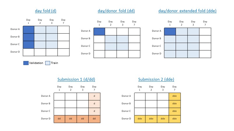\n\nAs you may notice, I didn’t bother about the LB range. I didn’t expect the absolute LB score to be of significance, so I only used it to check if CV improvements would translate to the LB. All methods provided good CV/LB correlation with one notable exception, which I suspected was caused by a bug.\n\n# Solution\n\n## Feature engineering\n\nI used combinations of the following input features in models optimized by Optuna:\n- Raw: This refers to the original input features. I noticed that several people asked for the actual raw data, which was made available at some point. I decided to forego using it, because my intuition was that it wouldn’t make a difference and it would save me precious time. Based on other writeups, my intuition might have been wrong.\n- PCA: input features reduced through PCA to up to 2048 principal components. Going beyond 2048 components didn’t seem to help. The PCA input was complemented by important features (borrowed from @ambrosm). I generated a version of PCA using all columns and another excluding important columns. I trained models using both the regular version of the PCA output and normalized versions. These latter versions didn’t seem to help, so I discarded them.\n- Type: cell type used only for cite. I theorized that I could build a good classification model to predict it for multi, but using the training data available didn’t seem to help CV.\n- Gender: donor gender\n- Day\n- KNN mean: mean value of input features for N nearest neighbors, reduced through PCA.\n- Mean: mean value of input features for donor/day, reduced through PCA. I used both the raw PCA and a normalized version.\n- Non-zero: mean number of non-zero features per cell for donor/day, reduced through PCA. Again, both the raw PCA and a normalized version.\n- Binary: input features converted to binary. My intuition was that the value matter less than whether the feature was present or not.\n\nContrary to my expectation, PCA input data performed better than raw data. It seems that it worked better to denoise data than other approaches I tried. After verifying that the public versions of important cite features helped training, I started using them, with the intention of conducting my own selection later. I never got to do it, though. Towards the end, I concluded I should have prioritized it.\n\nI used the following targets:\n- Raw: original targets\n- Binary: original targets converted to binary. I thought this would help denoise the target data without degrading performance (same intuition I applied to the input data). Although the correlation between the actual targets and the binary form was very high, this didn’t seem to help CV, so I discarded the approach.\n- PCA: original targets reduced through PCA to up to 2048 principal components. Training with a large number of components and using a smaller number for the prediction boosted the CV of individual models (up to 0.002, with the high end of the range seen in weaker models), but hindered ensembling.\n\nI tried these approaches independently and in combination, using multiple heads and loss functions. I discarded the combination models because the added complexity didn’t seem to help CV.\n\n# model architecture\n\nI used the following types of models:\n- NNs, mostly MLPs, residual networks, and 1dCNNs.\n- XGBD\n- ElasticNet\n\nNNs covered a range of options: dropout, normalization, gaussian noise, activation and others. For loss I used correlation, mse and binary cross entropy (for binary targets). I tried incorporating autoencoders into the models to denoise data, but it didn’t help CV. Non NN models performed clearly worse and didn’t even help with ensembling. With better tunning they might have helped with ensembling, but I never made that a priority.\n\nConceptually, this felt like a time series problem. However, as I understand it, the data collection process is intrusive and prevents us from having historical data for the same cell. I discarded using timeseries approaches given the small number of days we had and the risk of overfitting. In the last weekend, I tried enriching cell data with data from other cells for the same day/donor. This data was added as additional channels in a 3D input stream (batch, channel, features). I fed that to both LSTM and CNN models for a couple of dd folds with about the same results as my best existing models. With better tunning the results might have been different. Also, due to lack of time I only used the prediction of the first channel. I initially intended to ensemble the predictions from all channels as I theorized that the diversity would help. However, I wondered if it would offset the improvements of ensembling with other models, so I decided not to spend the time writing the corresponding code.\n\n# NLP Transformers\n\nIn my mind this problem is a classic case of language translation: from DNA to RNA, and from RNA to proteins. Transcription errors occur all the time and the measurement also introduces errors, hence the data ends up being noisy. I envisioned the following approach when I started the competition:\n- Assign a token to each input feature, to be defined as the column_number + a constant; build the input streams using the tokens of non zero features.\n- For multi, assign a token to each target column, to be defined as the column_number + a constant; build the target streams using the tokens of non zero columns.\n- Split the data in some way that makes sense to accommodate the maximum length limitations of the transformer. For example, for multi I intended to break data per chromosome and then merge the outputs. I had a few ideas for the merge, but wanted to see the output data before making a decision. My expectation was that each protein would be produced only by one of the chromosomes and that could facilitate the merging. In the cases in which the stream length for a chromosome was still too large, I'd further split it in partially overlapping segments, which the model would run through the transformer, to subsequently concatenate the outputs and run through the rest of the model;\n- Use any specific transformers for genetic data or regular ones for text (deberta, for example) and pretrain them with the competition data (e.g. MLM) or any other data publicly available (not needing tokens might facilitate that).\n- For multi, build both sequence-to-sequence models that take the binary input features and produce binary targets, and models that directly predict the value of each target column. For cite, use only the latter approach.\n- Depending on the performance of the transformer models, use their predictions directly in ensembling or to adjust the predictions of other models, e.g., merge both models and use the output of the transformer as a multiplier for the output of the other model, while also merging the losses of both models.\n\nLast Monday I finally gave it a go for multi. Given the limited time I had left, I went with a direct prediction of the target values using deberta. It didn’t take me long to write a draft version of the code, but I kept running into memory issues. I tried to work through them for a while, but it was late and after a week of not much sleep I sadly concluded that I had ran the clock. From the moment I started I was conscious that there wasn’t enough time left on that day to still use this approach in the competition, but I wanted to know if it would work.\n\n# ensembling\n\nI used linear regression on oof data for ensembling. I intended to use only the cells that better matched the PB sample but ended up discarding that idea, because the adversarial approach I used suggested that the vast majority of the training data was easily distinguishable from the PB data. To address the fact that the split of cells per day/donor was significantly different between training and LB, I balanced the oof data to have an equal number of cells per day/donor.\n\nAs mentioned earlier, I produced three sets of ensembles based respectively on d, dd and dde models. In the latter case, I excluded any models that used feature combinations that performed poorly with d and dd models, especially in the last day of the training data. A notable example were models using only PCA and day, which were the best performers for dde, but did poorly on d or dd. That suggested overfitting that would not generalize well to unseen days.\n\nThe following diagram summarizes the main characteristics of the models that compose my best solution (dde).\n\n\n\n# Final thoughts\n\nMy two final selections were an ensemble of dde models and an ensemble of merged d/dd models. The former performed better, but I suspect there is a problem with the merging of the d and dd ensembles. Out of curiosity, while writing this I submitted my best cite and multi models and got a 0.770982 PB score, which would rank 37th in the PB. Ensembling boosted it by +0.0012, which is consistent with what I measured with the CV. I should note though that the best cite model was not part of my selected ensemble. I’m pleased that I selected the ensemble with the highest PB score. I suspected there was going to be a big shakeup in the LB, except perhaps for the top positions, and for the most part that ended up happening. In the absence of any novel ideas, I credit my final position to strong fundamentals, particularly a solid CV strategy. That’s not what I expected to accomplish when I started, but I had a lot of fun participating in this competition and look forward to doing things differently, and hopefully better, next time.", "votes": 26 } ], "comments": [], "raw_markdown_by_id": { "2033231": "Thanks to Open Problems in Single-Cell Analysis and Kaggle for organizing this exciting competition. Ever since I was a little kid, I have had a passion for understanding how things worked. Three topics fascinate me the most: how the universe works (astrophysics and quantum mechanics), how the brain works (AI), and how life works (genetics and molecular biology). This competition was a wonderful opportunity to combine two of these topics. Unfortunately, I failed to live up to the expectations I had coming in. I was unable to come up with any good ideas with the potential to advance the field. Many years ago, I read a few books on genetics, starting with “Shadows of forgotten ancestors” (big Carl Sagan fan), but unfortunately, they are all very superficial on the science. I believe my illiteracy in the area was too big a handicap to overcome.\n\nI’d like to congratulate the winners and thank everyone who shared their knowledge and ideas, particularly @ambrosm, @psilogram and @pourchot. I’d also like to thank and commend @alexandervc for his contributions and tireless effort to motivate others and advance the science around the competition.\n\n# My journey\n\nUpon reading the competition description, looking at the data, reading some posts and browsing a couple of notebooks, I listed a set of ideas to try. At that stage, my hopes rested mainly on two of them: pseudo labeling unused test data and NLP transformer models. My plan was to build a strong model, generate pseudo labels, improve the model to get better labels, incorporate transformer models, gain a better understanding of the problem, come up with some breakthrough idea and have plenty of time to explore it. I knew that cite weighted more on the PB score, but I thought that multi’s low scores presented a better opportunity to differentiate. Despite having my sights on multi, I typically would build new code (create inputs, train, analyze results, predict, ensemble) first for cite and then adjust for multi. The thinking was that cite’s smaller data would make be easier to get the code right.\n\nThe need for a strong model to produce pseudo labels led to a big focus on ensembling, which I believe was detrimental to my performance. Also, the size of the data proved to be a much bigger challenge than I anticipated. Easily more than 90% of the time I dedicated to this competition was spent on trying to make things work within the memory available in Kaggle. It took me a while to build my first ensemble and conduct training with pseudo labels. The results were very disappointing. I wondered if it was because the model was generalizing better to unseen data, or if pseudo labeling just didn’t work. I spent some more time improving the base models and gave it another try, but with the same poor results.\n\nI then focused on a few other small improvements to my models, while building a more manageable overall pipeline (I broke processing in several pieces to deal with the memory and disk constraints). Then family demands and the need to revisit my analysis of several prospect investments during the recent stock market rout, ate away at my personal time. Before I knew it, the competition was over, and I hadn’t moved past the more fundamental stuff. If I were to do it again, I’d focus more on better understanding the science, better feature engineering and better individual models.\n\n# CV strategy\nThe CV strategy was the first thing I defined. The way I understood the problem, we had to make two types of predictions for which I devised two different CV approaches:\n\n| Prediction | CV method |\n| --- | --- |\n| Future day for 3 known donors | day (d): 3 folds based on day (4 for multi) |\n| Future day for an unknown donor | day/donor (dd): 9 folds based on day/donor (12 for multi). Training data excludes any records for the donor or day in the validation fold. |\n \nAlthough this strategy gave me confidence on the results, it had the downside of leaving a lot of data on the plate during training. I decided to edge this approach by using a variation of day/donor in which I would extend the training sample to any data that wasn’t for the same donor/day as the validation (dde). The downside of this approach is that it will overfit, and its results cannot be fully trusted. The upside is that it can lead to a better model as it uses more data. The following diagram illustrates the 3 methods, and how I used them for my two selected submissions.\n\n\n\nAs you may notice, I didn’t bother about the LB range. I didn’t expect the absolute LB score to be of significance, so I only used it to check if CV improvements would translate to the LB. All methods provided good CV/LB correlation with one notable exception, which I suspected was caused by a bug.\n\n# Solution\n\n## Feature engineering\n\nI used combinations of the following input features in models optimized by Optuna:\n- Raw: This refers to the original input features. I noticed that several people asked for the actual raw data, which was made available at some point. I decided to forego using it, because my intuition was that it wouldn’t make a difference and it would save me precious time. Based on other writeups, my intuition might have been wrong.\n- PCA: input features reduced through PCA to up to 2048 principal components. Going beyond 2048 components didn’t seem to help. The PCA input was complemented by important features (borrowed from @ambrosm). I generated a version of PCA using all columns and another excluding important columns. I trained models using both the regular version of the PCA output and normalized versions. These latter versions didn’t seem to help, so I discarded them.\n- Type: cell type used only for cite. I theorized that I could build a good classification model to predict it for multi, but using the training data available didn’t seem to help CV.\n- Gender: donor gender\n- Day\n- KNN mean: mean value of input features for N nearest neighbors, reduced through PCA.\n- Mean: mean value of input features for donor/day, reduced through PCA. I used both the raw PCA and a normalized version.\n- Non-zero: mean number of non-zero features per cell for donor/day, reduced through PCA. Again, both the raw PCA and a normalized version.\n- Binary: input features converted to binary. My intuition was that the value matter less than whether the feature was present or not.\n\nContrary to my expectation, PCA input data performed better than raw data. It seems that it worked better to denoise data than other approaches I tried. After verifying that the public versions of important cite features helped training, I started using them, with the intention of conducting my own selection later. I never got to do it, though. Towards the end, I concluded I should have prioritized it.\n\nI used the following targets:\n- Raw: original targets\n- Binary: original targets converted to binary. I thought this would help denoise the target data without degrading performance (same intuition I applied to the input data). Although the correlation between the actual targets and the binary form was very high, this didn’t seem to help CV, so I discarded the approach.\n- PCA: original targets reduced through PCA to up to 2048 principal components. Training with a large number of components and using a smaller number for the prediction boosted the CV of individual models (up to 0.002, with the high end of the range seen in weaker models), but hindered ensembling.\n\nI tried these approaches independently and in combination, using multiple heads and loss functions. I discarded the combination models because the added complexity didn’t seem to help CV.\n\n# model architecture\n\nI used the following types of models:\n- NNs, mostly MLPs, residual networks, and 1dCNNs.\n- XGBD\n- ElasticNet\n\nNNs covered a range of options: dropout, normalization, gaussian noise, activation and others. For loss I used correlation, mse and binary cross entropy (for binary targets). I tried incorporating autoencoders into the models to denoise data, but it didn’t help CV. Non NN models performed clearly worse and didn’t even help with ensembling. With better tunning they might have helped with ensembling, but I never made that a priority.\n\nConceptually, this felt like a time series problem. However, as I understand it, the data collection process is intrusive and prevents us from having historical data for the same cell. I discarded using timeseries approaches given the small number of days we had and the risk of overfitting. In the last weekend, I tried enriching cell data with data from other cells for the same day/donor. This data was added as additional channels in a 3D input stream (batch, channel, features). I fed that to both LSTM and CNN models for a couple of dd folds with about the same results as my best existing models. With better tunning the results might have been different. Also, due to lack of time I only used the prediction of the first channel. I initially intended to ensemble the predictions from all channels as I theorized that the diversity would help. However, I wondered if it would offset the improvements of ensembling with other models, so I decided not to spend the time writing the corresponding code.\n\n# NLP Transformers\n\nIn my mind this problem is a classic case of language translation: from DNA to RNA, and from RNA to proteins. Transcription errors occur all the time and the measurement also introduces errors, hence the data ends up being noisy. I envisioned the following approach when I started the competition:\n- Assign a token to each input feature, to be defined as the column_number + a constant; build the input streams using the tokens of non zero features.\n- For multi, assign a token to each target column, to be defined as the column_number + a constant; build the target streams using the tokens of non zero columns.\n- Split the data in some way that makes sense to accommodate the maximum length limitations of the transformer. For example, for multi I intended to break data per chromosome and then merge the outputs. I had a few ideas for the merge, but wanted to see the output data before making a decision. My expectation was that each protein would be produced only by one of the chromosomes and that could facilitate the merging. In the cases in which the stream length for a chromosome was still too large, I'd further split it in partially overlapping segments, which the model would run through the transformer, to subsequently concatenate the outputs and run through the rest of the model;\n- Use any specific transformers for genetic data or regular ones for text (deberta, for example) and pretrain them with the competition data (e.g. MLM) or any other data publicly available (not needing tokens might facilitate that).\n- For multi, build both sequence-to-sequence models that take the binary input features and produce binary targets, and models that directly predict the value of each target column. For cite, use only the latter approach.\n- Depending on the performance of the transformer models, use their predictions directly in ensembling or to adjust the predictions of other models, e.g., merge both models and use the output of the transformer as a multiplier for the output of the other model, while also merging the losses of both models.\n\nLast Monday I finally gave it a go for multi. Given the limited time I had left, I went with a direct prediction of the target values using deberta. It didn’t take me long to write a draft version of the code, but I kept running into memory issues. I tried to work through them for a while, but it was late and after a week of not much sleep I sadly concluded that I had ran the clock. From the moment I started I was conscious that there wasn’t enough time left on that day to still use this approach in the competition, but I wanted to know if it would work.\n\n# ensembling\n\nI used linear regression on oof data for ensembling. I intended to use only the cells that better matched the PB sample but ended up discarding that idea, because the adversarial approach I used suggested that the vast majority of the training data was easily distinguishable from the PB data. To address the fact that the split of cells per day/donor was significantly different between training and LB, I balanced the oof data to have an equal number of cells per day/donor.\n\nAs mentioned earlier, I produced three sets of ensembles based respectively on d, dd and dde models. In the latter case, I excluded any models that used feature combinations that performed poorly with d and dd models, especially in the last day of the training data. A notable example were models using only PCA and day, which were the best performers for dde, but did poorly on d or dd. That suggested overfitting that would not generalize well to unseen days.\n\nThe following diagram summarizes the main characteristics of the models that compose my best solution (dde).\n\n\n\n# Final thoughts\n\nMy two final selections were an ensemble of dde models and an ensemble of merged d/dd models. The former performed better, but I suspect there is a problem with the merging of the d and dd ensembles. Out of curiosity, while writing this I submitted my best cite and multi models and got a 0.770982 PB score, which would rank 37th in the PB. Ensembling boosted it by +0.0012, which is consistent with what I measured with the CV. I should note though that the best cite model was not part of my selected ensemble. I’m pleased that I selected the ensemble with the highest PB score. I suspected there was going to be a big shakeup in the LB, except perhaps for the top positions, and for the most part that ended up happening. In the absence of any novel ideas, I credit my final position to strong fundamentals, particularly a solid CV strategy. That’s not what I expected to accomplish when I started, but I had a lot of fun participating in this competition and look forward to doing things differently, and hopefully better, next time." } }