{"cells":[{"metadata":{},"cell_type":"markdown","source":"# Strides Towards Safety \n### NFL 1st and Future - Playing Surface Analytics - Submission by Katherine Lordi"},{"metadata":{},"cell_type":"markdown","source":"# My Findings \nGiven the provided [datasets](http://https://www.kaggle.com/c/nfl-playing-surface-analytics/data), I found specific player movement patterns that may present an elevated risk of acute onset of injury in NFL athletes. \n### *Metrics of Player Movement That May Influence Risk of Injury:*\n#### 1) Frequency of Slows/Stops: When players slow to speeds near 0 (or completely stop) more frequently, they may be at greater risk for injuries on Synthetic Turf than Natural Grass on average. \n* On average, number of slows/stops per sec for injuries was higher on Synthetic Turf than Natural Grass by 30%. \n\n#### 2) Frequency of Changes of Direction: When players change their direction more frequently, they may be at greater risk for injuries on Synthetic Turf than Natural Grass on average. \n- On average, number of changes in direction per sec for injuries was higher on Synthetic Turf than Natural Grass by 37%. \n\n#### 3) Frequency of Changes of Orientation: When players change their orientation (turn or pivot) more frequently, they may be at greater risk for injuries on Synthetic Turf than Natural Grass on average.\n- On average, number of changes in orientation per sec for injuries was higher on Synthetic Turf than Natural Grass by 63%. \n\n#### 4) Differences in Metrics Across Playing Surfaces for Non-Injuries: For the non-injured player population, I found that the metrics of player movement that may influence risk of injury (frequencies of slows/stops, change in direction, and change in orientation) do not differ across playing surfaces. \n\n### *How Player Movement and Game Environment Interact to Influence Risk of Injury :*\n#### 1) On average in outdoor stadiums, severity of injuries that occur on synthetic turf was 87% higher than natural grass.\n- Holds across player movement metrics (frequency of slows/stops, direction, orientation) that may influence risk of injury\n- Looked at play types with the most injuries (ex. pass punt)\n- Looked at positions with the most injuries (ex. WR) \n\n### *Extensions of My Findings to Next Gen Stats to Help Safety Efforts*\nBased on my findings above and my attempt at having a decision tree model classify things such as field type and DM from the data, here are some ideas to help reduce lower extremity injuries in the NFL, the highest driver of days missed by players. \n#### Incorporate these player movement metrics into AI models aiming to predict and prevent injury \n- Frequency of slows/slops, direction and orientation changes\n- Other historical player-specific and game-level data \n\n#### Look at these player movement metrics in conjunction with specific types of cleats, grass and synthetic fields and incorporate into AI models \n- Cleat Tracking Technology \n- Injury Rates Per Cleat \n\n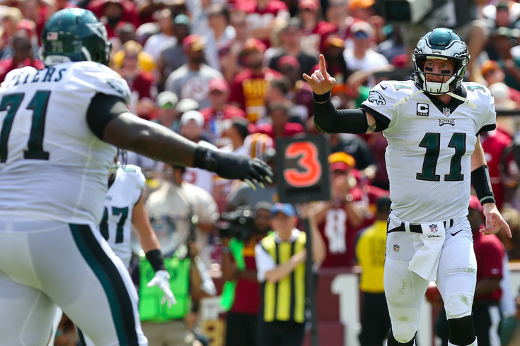\nLower extremity injuries such as ACL tears and Achilles tendon ruptures are two of the most serious season-ending injuries ([Bleacher Report](http://bleacherreport.com/articles/2089798-how-and-why-minimal-or-non-contact-injuries-occur-in-nfl-workouts)). Carson Wentz (QB) and Jason Peters (T) of the Philadelphia Eagles suffered season-ending knee injuries prior to the Eagles Super Bowl LII win. \n"},{"metadata":{},"cell_type":"markdown","source":"# Contents \n* [My Findings](#1) \n* [Challenge & Dataset](#2)\n* [Overview of My Process](#3)\n* [1) Preprocessing the Data](#4) \n* [2) Understanding the Data: Preliminary Visualizations of Injuries](#5)\n* [3) Visualizing Player Movement](#6)\n* [4) Preprocessing Player Tracking Data: Flattening the Data](#7)\n* [5) A Look at Player Movement: Slows/Stops, Direction, Orientation](#8)\n* [6) A Look at Outdoor Stadiums](#9)\n* [7) Decision Tree to Predict Injury](#10)\n* [8) Extensions to Next Gen Stats](#11)"},{"metadata":{},"cell_type":"markdown","source":"# Overview: Challenge & Dataset \n\n#### **The Challenge:** To characterize differences in player movement between the natural grass and synthetic turf and identify specific variables that may influence player movement and the risk of injury. For the analysis, we used [3 data files](https://www.kaggle.com/c/nfl-playing-surface-analytics/data) that are linked using the fields PlayerKey, GameID, and PlayKey. \n\n- **InjuryRecord:** Contains 105 lower-limb non-contact injuries, location in the body, field type the injury occurred, and severity based on # days a player missed during regular season games over two seasons.\n- **PlayList:** Contains details for the 267,005 player-plays including the player’s roster and play positions, stadium type, field type, weather, and play type.\n- **PlayerTrackerData:** Contains 76,366,748 data points of player tracking data via [Next Gen Stats](https://nextgenstats.nfl.com/) that describe the location, orientation, speed, and direction of each player during a play. 10 observations were recorded per second. \n\n### Data Constraints \nWith these three files, we have information about the injuries, inflicted player (position, day #, game #), tracking data on the field, play type, and environment (playing surface, environment, temperature). However, here are some constraints that I took into consideration: \n- We only have data on 105 non-contact lower limb injuries that occurred in 267,005 plays (0.039% of plays have a non-contact lower-limb injury)\n- When exactly in the play does the injury occur? \n- What kind of injury is it exactly? (ie. ankle sprain, ACL tear, etc.) \n- Name? Age? Years Active in the NFL? Height? Weight? Teams? Players are more than just a PlayerKey. \n- What is the player's injury history? Is the player suffering or recovering from any other injuries? Having other injuries certainly impacts health and the potential for future injuries.\n- Not all players play the same # of games on the same types of fields\n- Specifics about type of cleats differ for many players across natural grass VS synthetic turf \n- Type of playing surface that a player and team practices on\n- Home Field playing surface \n- How often a player plays on natural grass VS synthetic turf \n- Player preferences for playing surface \n- etc. \n\nThe above points are limitations of our dataset, and player factors such as these certainly play a major role in understanding player biomechanics and potential risks for injury. However, rather than focusing on biomechanics and these factors, **we focus on examining player movement itself on synthetic turf and natural grass** and **variables that may influence movements and risk of injury** such as player tracking data and environmental/game variables such as weather, temperature, play type, etc. "},{"metadata":{},"cell_type":"markdown","source":"# Overview: My Process \nIn football, there is so much variability in player movement that differs across every single play across so many game and environmental variables. For example, Wide Receivers (WR) constantly change their speed and direction to get open, and Cornerbacks (CB) that defend them quickly anticipate their movements to prevent them from catching a pass. Additionally, we only have 105 non-contact lower limb injuries total, so these injuries are pretty rare. \n\nAfter doing my preliminary analysis of the data, I saw that there were no significant correlations between player tracking data (player's x and y position on the field, speed, acceleration, orientation, and direction) and environmental/game variables to injuries on different field types. Understanding that no playing surface is perfect (but there is [NFL Field Certification](https://operations.nfl.com/the-game/game-day-behind-the-scenes/nfl-field-certification/)!) and given 2 years of Player Tracking Data, I sought dive deeper into understanding player movements such as rates and frequencies of sudden stops, directional changes, and orientation changes in order to understand how they relate to risk of injury. In this notebook, I show my process and the notable visualizations that helped me get to my findings. "},{"metadata":{},"cell_type":"markdown","source":"# 1) Preprocessing The Data \nFirst, I import the files and joined InjuryRecord with PlayList into one file in order to visualize relationships between factors such as injury location, severity, play type, field type, position, weather, temperature, etc. "},{"metadata":{"_kg_hide-output":true,"trusted":true,"_kg_hide-input":true},"cell_type":"code","source":"import pandas as pd\nimport matplotlib.pyplot as plt\nfrom sklearn.tree import DecisionTreeClassifier\nfrom sklearn.model_selection import train_test_split\nfrom sklearn import metrics\nfrom sklearn.tree import export_graphviz\nfrom sklearn.externals.six import StringIO\nfrom IPython.display import Image\nimport seaborn as sns \nimport numpy as np","execution_count":null,"outputs":[]},{"metadata":{"trusted":true,"_kg_hide-input":true},"cell_type":"code","source":"# Import Data Files and display length \nir = pd.read_csv(\"../input/nfl-playing-surface-analytics/InjuryRecord.csv\")\npl = pd.read_csv(\"../input/nfl-playing-surface-analytics/PlayList.csv\").set_index(\"PlayKey\")\nptd = pd.read_csv(\"../input/nfl-playing-surface-analytics/PlayerTrackData.csv\").set_index(\"PlayKey\")\nl1 = len(ir)\nl2 = len(pl)\nl3 = len(ptd)\nprint(\"Length of InjuryRecord is \", l1)\nprint(\"Length of PlayList is \", l2)\nprint(\"Length of PlayerTrackData is \", l3)","execution_count":null,"outputs":[]},{"metadata":{},"cell_type":"markdown","source":"I also modified InjuryRecord by adding the appropriate missing values in the PlayKey column and merging the multiple DM (Days Missed) columns indicating severity into one column for simplicity. Therefore, DM = 1 means 1+ days missed while a DM = 42 means 42 + days missed. See the head of this file below. "},{"metadata":{"_kg_hide-input":true,"trusted":true,"_kg_hide-output":false},"cell_type":"code","source":"# Modifying InjuryRecord: Adding PlayKey for missing rows and Merging DM columns (indicate severity) into one column. \ndef fdm(d):\n DM=[1,7,28,42]\n return DM[d-1] if d else 0\n\nir = ir.fillna(\"*\")\n\nir['dmi'] = ir['DM_M1'] + ir['DM_M7'] + ir['DM_M28'] + ir['DM_M42']\nir['DM'] = ir['dmi'].apply(fdm)\n\ngidpk = {}\nfor gid in ir.query('PlayKey == \"*\"').GameID:\n gidpk[gid] = pl.query('GameID==\"%s\"' % gid).index[-1]\n\n\ndef fpku(a,b):\n return gidpk[b] if a == \"*\" else a\n\nir['PlayKey'] = ir.apply(lambda x: fpku(x.PlayKey, x.GameID), axis=1)\n\nInjuryRecord = ir.set_index(\"PlayKey\")[['BodyPart','DM']]\nInjuryRecord.head()","execution_count":null,"outputs":[]},{"metadata":{},"cell_type":"markdown","source":"Next, I joined InjuryRecord and PlayList into a new file and then check to ensure that the # of injuries in this file is 105."},{"metadata":{"trusted":true,"_kg_hide-output":true,"_kg_hide-input":true},"cell_type":"code","source":"# joining InjuryRecord and PlayList \nIRPL = pl.join(InjuryRecord).fillna(0)\nIRPL.head()","execution_count":null,"outputs":[]},{"metadata":{"_kg_hide-input":true,"trusted":true,"_kg_hide-output":true},"cell_type":"code","source":"# does a check to ensure that the # of injuries in the dataset is 105. \nIRPL.query('DM > 0').count()","execution_count":null,"outputs":[]},{"metadata":{},"cell_type":"markdown","source":"# 2) Understanding the Data: Preliminary Visualizations \nFirst, I looked at some tables and visualizations in order to better understand the data, visualize relationships, brainstorm ideas, and guide my next steps. \n\n### Injuries by Body Part and Field Type \nThe graphs below visualize the distribution of injury type on each playing surface and how severity differed across the playing surfaces. Some things to note are:\n- Knee and ankle injuries are the most common. \n- There are an equal number of knee injuries on synthetic turf and natural grass (24). \n- There are more ankle injuries on synthetic turf (25) than natural grass (17). \n- There are more foot injuries on natural grass than synthetic turf.\n- There are more toe injuries on synthetic turf than natural grass.\n- Ankle injuries are more severe (more days missed) on synthetic turf than natural grass. "},{"metadata":{"_kg_hide-input":true,"trusted":true},"cell_type":"code","source":"fig = plt.figure(figsize=(20,16))\nax1 = fig.add_subplot(221)\nax2 = fig.add_subplot(222)\nax3 = fig.add_subplot(223)\nax4 = fig.add_subplot(224)\nax1.set_title('# Injuries by Body Part')\nax1.set_ylabel('Count')\nax1.set_xlabel('Body Part')\nax2.set_title('# Injuries by Field Type')\nax2.set_ylabel('Count')\nax2.set_xlabel('Body Part')\nax3.set_title('# Natural Grass: Injuries by Body Part by Severity')\nax3.set_ylabel('Count')\nax3.set_xlabel('Body Part')\nax3.set_ylim(0,12)\nax4.set_title('# Synthetic Turf: Injuries by Body Part by Severity')\nax4.set_ylabel('Count')\nax4.set_xlabel('Body Part')\nax4.set_ylim(0,12)\nplot1 = IRPL.query('DM>0').pivot_table(index=['BodyPart'], columns=[], values='DM', aggfunc='count').fillna(0).plot(kind='bar',ax=ax1,legend=False)\nplot2 = IRPL.query('DM>0').pivot_table(index=['BodyPart'], columns=['FieldType'], values='DM', aggfunc='count').fillna(0).plot(kind='bar',ax=ax2)\nplot3 = IRPL.query('DM>0 and FieldType == \"Natural\"').pivot_table(index=['BodyPart'], columns=['DM'], values='PlayerKey', aggfunc='count').fillna(0).plot(kind='bar',ax=ax3)\nplot4 = IRPL.query('DM>0 and FieldType == \"Synthetic\"').pivot_table(index=['BodyPart'], columns=['DM'], values='PlayerKey', aggfunc='count').fillna(0).plot(kind='bar',ax=ax4)","execution_count":null,"outputs":[]},{"metadata":{},"cell_type":"markdown","source":"### Injuries By Position, Field Type, Severity, & Play Type \nThe graph below shows positions with an injury by body part. We notice the following in the graph below:\n- Wide Receivers (WR) see the most non-contact ankle and knee injuries.\n- Cornerbacks (CB) have the most ankle and knee injuries of the DB Position Group.\n- Offensive Linebackers (OLB) see the second highest # of knee injuries (next to WR) and also a notable number of ankle injuries. \n- Running Backs (RB) also see greater amounts of non-contact knee injuries than other positions but have fewer ankle injuries. \n"},{"metadata":{"trusted":true,"_kg_hide-input":true},"cell_type":"code","source":"fig = plt.figure(figsize=(12,4))\nax1 = fig.add_subplot(111)\nax1.set_title('# Injuries by Position and Body Part')\nax1.set_ylabel('Count')\nax1.set_xlabel('Position Group, Position')\nIRPL.query('DM>0').pivot_table(index=['PositionGroup','Position'], columns=['BodyPart'], values='DM', aggfunc='count').fillna(0).plot(kind='bar', ax = ax1)\nplt.show()","execution_count":null,"outputs":[]},{"metadata":{},"cell_type":"markdown","source":"Next, I looked at injuries through the perspective of field type and severity. In the table below, count indicates injuries by the # while sum indicates injuries by severity (DM == Days Missed). I noticed the following that can be seen in the table below:\n- Cornerbacks (CB) only have ankle injuries on synthetic turf (7) and report 0 ankle injuries on natural grass. \n- Strong Safeties (SS) only have ankle injuries on synthetic turf (3) and report 0 ankle injuries on natural grass. \n- Wide Receivers (WR) have 5 ankle injuries on natural grass and 4 on synthetic turf. \n- There are an equal number of knee injuries on synthetic turf and natural grass. "},{"metadata":{"_kg_hide-input":true,"trusted":true,"_kg_hide-output":true},"cell_type":"code","source":"IRPL.query('DM>0').pivot_table(index=['PositionGroup', 'Position','FieldType'], columns=['BodyPart'], values='DM',aggfunc=['count', 'sum']).fillna(0)","execution_count":null,"outputs":[]},{"metadata":{},"cell_type":"markdown","source":"I also looked at injuries through the perspective of field type and play type. I noticed the following major significances that can be seen in the table and graph below:\n- Pass and rush plays have the most injuries. \n- The most knee injuries occurred during a pass (10 natural, 10 synthetic) followed by rush (5 natural, 5 synthetic) and then kickoff (4 natural, 3 synthetic), and punt (4 natural, 2 synthetic). \n- The most ankle injuries occurred during a pass (7 natural, 14 synthetic --> largest discrepancy) followed by rush (7 natural, 7 synthetic), kickoff, and then punt. "},{"metadata":{"trusted":true,"_kg_hide-input":true,"_kg_hide-output":true},"cell_type":"code","source":"IRPL.query('DM>0').pivot_table(index=['PlayType', 'FieldType'], columns=['BodyPart'], values='DM',aggfunc=['count', 'sum']).fillna(0)","execution_count":null,"outputs":[]},{"metadata":{"trusted":true,"_kg_hide-input":true},"cell_type":"code","source":"fig = plt.figure(figsize=(12,4))\nax1 = fig.add_subplot(111)\nax1.set_title('# Injuries by Play Type and Body Part')\nax1.set_ylabel('Count')\nax1.set_xlabel('Play Type')\nIRPL.query('DM>0').pivot_table(index=['PlayType'], columns=['BodyPart'], values='DM', aggfunc='count').fillna(0).plot(kind='bar', ax = ax1)\nplt.show()","execution_count":null,"outputs":[]},{"metadata":{},"cell_type":"markdown","source":"It is difficult to speculate a lot from the above tables about WHY certain positions and play types have different numbers of injuries in differerent body parts based on the playing surface. Therefore, my next step was to look at correlations between data variables and analyze player movements using the Player Tracking Data. "},{"metadata":{},"cell_type":"markdown","source":"### Correlations Between Injuries and PlayList Columns (Field Type, StadiumType, Temperature, Weather, PlayType, Position)\n\nI made a correlation heat map to see if there are any obvious correlations between injuries and game/player variables. After seeing no correlations, I dove into trying to analyze player movements using the Player Tracking Data since 2 seasons worth was provided. "},{"metadata":{"_kg_hide-input":true,"trusted":true},"cell_type":"code","source":"def ftoint(d):\n l = list(set(d))\n ld = {l[k]:k for k in range(len(l))}\n\n def fmap(x):\n return ld[x]\n \n return fmap\n\ndef fint(s, k):\n f = ftoint(IRPL[s])\n IRPL[k] = IRPL[s].apply(f)","execution_count":null,"outputs":[]},{"metadata":{"_kg_hide-input":true,"trusted":true},"cell_type":"code","source":"fint('RosterPosition', 'irp')\nfint('StadiumType', 'istadium')\nfint('FieldType', 'ifield')\nfint('Weather', 'iweather')\nfint('PlayType', 'iplay')\nfint('Position', 'iposition')\nfint('PositionGroup', 'igroup')\nfint('BodyPart', 'ibody')\n\nfig = plt.figure(figsize=(20,20))\nax1 = fig.add_subplot(221)\nax2 = fig.add_subplot(222)\nax1.set_title('Heat Map of Correlations of Features to Injury')\nax2.set_title('Heat Map of Correlations of Features')\nsns.heatmap(IRPL.query('DM > 0')[['PlayerDay','PlayerGame','PlayerGamePlay','Temperature','iweather','ifield','istadium','iposition','igroup','ibody']].corr(),ax=ax1)\nsns.heatmap(IRPL[['PlayerDay','PlayerGame','PlayerGamePlay','Temperature','iweather','ifield','istadium','iposition','igroup','ibody']].corr(),ax=ax2)\nplt.show()","execution_count":null,"outputs":[]},{"metadata":{},"cell_type":"markdown","source":"# 3) Visualizing Player Movement \nI did some visualizations of Player Movement using the Player Tracking Data in order to see how different positions move on the field. In these graphs of the player's direction, change in direction, velocity, and change in orientation over time, we can better understand how the player is moving on the field."},{"metadata":{"trusted":true,"_kg_hide-input":false},"cell_type":"code","source":"# Change this to change the player and play being looked at: \nPLAYER='43518'\nPK='43518-6-25'","execution_count":null,"outputs":[]},{"metadata":{"trusted":true},"cell_type":"code","source":"PK0 = IRPL.query('PlayerKey==%s' % PLAYER).index[0]\nPKN = IRPL.query('PlayerKey==%s' % PLAYER).index[-1]\n(PK0, PKN)\n\ndf1 = ptd[PK0:PKN]\ndf2 = IRPL[PK0:PKN]\n\ndf = df1.join(df2).fillna(0)\n\ndf['rdir'] = df['dir'] * np.pi / 180.\n\nPK = '43518-1-12'\ndfx = df.query('PlayKey == \"%s\"' % PK).reset_index().set_index('time')\n\nfunwrap = lambda c : np.unwrap(dfx[c], discont=180.)\nfdiff = lambda c : abs(dfx[[c]].diff(axis=0).fillna(0))\n\ndfx['udir'] = funwrap('dir')\ndfx['vudir'] = fdiff('udir')\n\ndfx['uo'] = funwrap('o')\ndfx['vuo'] = fdiff('uo')\n","execution_count":null,"outputs":[]},{"metadata":{"_kg_hide-input":true,"_kg_hide-output":true,"trusted":true},"cell_type":"code","source":"fbins = lambda c, b : pd.cut(x=dfx[c], bins=b, labels=b[1:])\nsbins = [0., 0.01, 0.05, 0.1, 0.2, 0.3, 0.4, 0.5, 1.0, 5.0 ]\nscols = ['cs_%d' % int(i*100) for i in sbins[1:] ]\ndfx['s_bin'] = fbins('s', sbins)\n\nbins = [0,30,60,90,120,150,180,360]\ncols1 = ['cdir_%d' % i for i in bins[1:]]\ndfx['vudir_bin'] = fbins('vudir', bins)\n\ncols2 = ['co_%d' % i for i in bins[1:]]\ndfx['vuo_bin'] = fbins('vuo', bins)\n\nfzip = lambda c, h : dict(zip(h, list(dfx.groupby(c)[c].count())))\n\nx = fzip('vudir_bin', cols1)\nx.update(fzip('vuo_bin', cols2))\nx.update(fzip('s_bin', scols))\n\n#dfx.groupby('s_bin')['s_bin'].count()","execution_count":null,"outputs":[]},{"metadata":{"_kg_hide-input":true,"trusted":true,"_kg_hide-output":false},"cell_type":"code","source":"x = dfx.groupby('vudir_bin')['vudir_bin'].count()\ncols = ['cdir_%d' % i for i in bins[1:]]\n(cols,list(x))\n\ndict(zip(cols,list(x)))\n\nfig = plt.figure(figsize=(20,12))\nax1 = fig.add_subplot(221)\nax2 = fig.add_subplot(222)\nax3 = fig.add_subplot(223)\nax4 = fig.add_subplot(224)\n\nax1.set_title('Player Direction Over Time')\nax1.set_ylabel('Degrees')\nax1.set_xlabel('time (sec)')\nax2.set_title('Change in Direction Over Time')\nax2.set_ylabel('Degrees')\nax2.set_xlabel('time (sec)')\nax3.set_title('Player Velocity Over Time')\nax3.set_ylabel('yards/sec')\nax3.set_xlabel('time (sec)')\nax4.set_title('Change in Orientation Over Time')\nax4.set_ylabel('degrees')\nax4.set_xlabel('time (sec)')\nax4.set_ylim(-90,90)\n\n\ndfx['udir'].plot(ax=ax1)\ndfx['vudir'].plot(ax=ax2)\ndfx['s'].plot(ax=ax3)\ndfx['vuo'].plot(ax=ax4)\ndfx.query('s_bin <= 0.05')['s'].plot(style='.', ax=ax3)\nplt.show()","execution_count":null,"outputs":[]},{"metadata":{},"cell_type":"markdown","source":"# 4) Preprocessing Player Tracking Data: Flattening the Data \nAfter visualizing player movement in different ways, I hypothesized that when players are constantly shifting their direction, orientation, speed, and making cuts on the field that they may be at greater risk of lower limb injuries. I identified the following variables of interest: change in direction, change in orientation, changes in speed near 0. \n\nSince Player Tracking Data is so large and each row represents .10 seconds of a play, I decided to flatten it in order to decrease the amount of data points to one data point per play. I did the following when flattening the Player Tracking Data:\n- Classified changes in direction and orientation by binning in 30 degree buckets\n- Characterized velocity in the x and y direction by binning in buckets of 0.01 yards/second to 5 yards/second. \n\nSee the code for flattening the data below (do not run it I load the file in after): "},{"metadata":{"trusted":true,"collapsed":true,"_kg_hide-input":true,"_kg_hide-output":true},"cell_type":"code","source":"# Flattening Player Tracking Data in order to decrease the amount of data points to one data point per play\n# Classified changes in direction and orientation by binning in 30 degree buckets\n# Characterized velocity in the x and y direction by binning in buckets of 0.01 yards/second to 5 yards/second. \n\nclass Play(object):\n \n def __init__(self):\n self.header=list(pd.read_csv(\"../input/nfl-playing-surface-analytics/PlayerTrackData.csv\",nrows=2).keys())\n self.current_play_df = None\n self.next_row = 1\n \n def get_play1(self):\n dft_prev = None\n n = 0\n for df in pd.read_csv(\"../input/nfl-playing-surface-analytics/PlayerTrackData.csv\",names=self.header,chunksize=1000,skiprows=1):\n n = n + 1\n dfc = df[['PlayKey']]\n pkeys_j = dfc.ne(dfc.shift()).apply(lambda x: x.index[x].tolist())\n pkeys = [dfc.PlayKey[j] for j in pkeys_j[0]]\n for playkey in pkeys[0:-1]:\n if dft_prev is None:\n dft = df.query('PlayKey == \"%s\"' % playkey)\n else:\n dft = dft_prev.append(df.query('PlayKey == \"%s\"' % playkey))\n dft_prev = None\n \n yield dft.reset_index()\n \n dft_prev = df.query('PlayKey == \"%s\"' % pkeys[-1])\n \n \n def next_play(self):\n dft = pd.read_csv(\"../input/nfl-playing-surface-analytics/PlayerTrackData.csv\",names=header,skiprows=self.next_row,nrows=1000)\n playkey = dft.PlayKey[0]\n self.current_play_df = dft.query('PlayKey == \"%s\"' % playkey)\n l = len(self.current_play_df.PlayKey)\n self.next_row = self.next_row + l\n return self.current_play_df\n \n def get_playkey(self):\n return self.current_play_df.PlayKey[0]\n \n def get_events(self):\n return set(self.current_play_df.event)\n \n def get_plays(self, n):\n \n sbins = [0., 0.01, 0.05, 0.1, 0.2, 0.3, 0.4, 0.5, 1.0, 5.0 ]\n scols = ['cs_%d' % int(i*100) for i in sbins[1:] ]\n scolsx = ['cvx_%d' % int(i*100) for i in sbins[1:] ]\n scolsy = ['cvy_%d' % int(i*100) for i in sbins[1:] ]\n \n bins = [0,30,60,90,120,150,180,360]\n cols1 = ['cdir_%d' % i for i in bins[1:]] \n cols2 = ['co_%d' % i for i in bins[1:]] \n\n funwrap = lambda dfx, c : np.unwrap(dfx[c], discont=180.)\n fdiff = lambda dfx, c : abs(dfx[[c]].diff(axis=0).fillna(0))\n fbins = lambda dfx, c, b : pd.cut(x=dfx[c], bins=b, labels=b[1:])\n fzip = lambda dfx, c, h : dict(zip(h, list(dfx.groupby(c)[c].count())))\n \n data = []\n t0 = datetime.now()\n i = 0\n for df in self.get_play1():\n d = {'PlayKey': df.PlayKey[0]}\n last = len(df) - 1\n d['Events'] = list(set(df.event))\n d['Duration'] = df.time[last]\n d['TotalDis'] = df.dis.sum()\n \n df1 = df.set_index('time')\n df1['udir'] = funwrap(df1, 'dir')\n df1['vudir'] = fdiff(df1, 'udir') \n df1['uo'] = funwrap(df1, 'o')\n df1['vuo'] = fdiff(df1, 'uo')\n \n df1['vx'] = fdiff(df1, 'x')\n df1['vy'] = fdiff(df1, 'y')\n \n df1['vx_bin'] = fbins(df1, 'vx', sbins)\n df1['vy_bin'] = fbins(df1, 'vy', sbins)\n\n df1['vudir_bin'] = fbins(df1, 'vudir', bins)\n df1['vuo_bin'] = fbins(df1, 'vuo', bins)\n \n d.update(fzip(df1, 'vudir_bin', cols1))\n d.update(fzip(df1, 'vuo_bin', cols2))\n d.update(fzip(df1, 'vx_bin', scolsx))\n d.update(fzip(df1, 'vy_bin', scolsy))\n \n data.append(d)\n i = i + 1\n if i%10000 == 0:\n t1 = datetime.now()\n print(i,t1-t0)\n t0=t1\n if i >= n: break\n return data\n \n\nprint(\"Start:\", datetime.now())\nplay = Play()\ndata = play.get_plays(300000)\ndfplays = pd.DataFrame(data).set_index('PlayKey')\nprint(\"End:\", datetime.now())\n\ndfplays.to_parquet('plays4.parquet', compression='GZIP')\ndfplays.to_csv('plays4.csv')\ndf = dfpi.join(dfplays).fillna(0)\ndf.to_csv(\"df1.csv\")","execution_count":null,"outputs":[]},{"metadata":{},"cell_type":"markdown","source":"After flattening the Player Tracking Data, I had counts of changes in speed to near 0, direction, and orientation by the count. However, I realized that counts can vary greatly depending on the duration of the play. Therefore, I created new columns for the following in order to normalize the data:\n- change in direction per second: cdir_rate\n- change in orientation per second: co_rate\n- change in speed to a slow or stop per second: cvx_rate and cvy_rate "},{"metadata":{"_kg_hide-input":true,"_kg_hide-output":true,"trusted":true},"cell_type":"code","source":"ptd2 = pd.read_csv(\"../input/joined2/df2.csv\")\n#ptd2.keys()","execution_count":null,"outputs":[]},{"metadata":{"_kg_hide-input":true,"trusted":true},"cell_type":"code","source":"ptd2['cdir_total'] = ptd2['cdir_60'] + ptd2['cdir_90'] + ptd2['cdir_120'] + ptd2['cdir_150'] + ptd2['cdir_180']\nptd2['co_total'] = ptd2['co_60'] + ptd2['co_90'] + ptd2['co_120'] + ptd2['co_150'] + ptd2['co_180']\nptd2['cdir_rate'] = ptd2['cdir_total'] / ptd2['Duration']\nptd2['co_rate'] = ptd2['co_total'] / ptd2['Duration']\nptd2['sum_vx'] = ptd2['cvx_1'] + ptd2['cvx_5'] + ptd2['cvx_10'] + ptd2['cvx_20'] + ptd2['cvx_30'] + ptd2['cvx_40'] + ptd2['cvx_50'] + ptd2['cvx_100'] + ptd2['cvx_500'] \nptd2['sum_vy'] = ptd2['cvy_1'] + ptd2['cvy_5'] + ptd2['cvy_10'] + ptd2['cvy_20'] + ptd2['cvy_30'] + ptd2['cvy_40'] + ptd2['cvy_50'] + ptd2['cvy_100'] + ptd2['cvy_500'] \nptd2['cvx_rate'] = ptd2['cvx_1'] / ptd2['Duration']\nptd2['cvy_rate'] = ptd2['cvy_1'] / ptd2['Duration']\nptd2['avg_velocity'] = ptd2['TotalDis'] / ptd2['Duration']\nptd2.head()","execution_count":null,"outputs":[]},{"metadata":{},"cell_type":"markdown","source":"# 5) A Look at Player Movement: Slows/Stops, Direction, Orientation \nLooking at the graphs below and also converting them into tables to see the actual values, I found that frequency of slows and stops, changes in direction, and changes in orientation may influence risk of injury on average. I compared graphs with the average frequencies across the injured and non-injured population."},{"metadata":{"trusted":true,"_kg_hide-input":true},"cell_type":"code","source":"fig = plt.figure(figsize=(20,18))\nax1 = fig.add_subplot(321)\nax2 = fig.add_subplot(322)\nax3 = fig.add_subplot(323)\nax4 = fig.add_subplot(324)\nax5 = fig.add_subplot(325)\nax6 = fig.add_subplot(326)\n\nax1.set_title('Injury: Average # Slows/Stops per Second')\nax1.set_ylabel('Average')\nax1.set_xlabel('Field Type')\nax1.set_ylim(0,1)\n\nax2.set_title('No Injury: Average # Slows/Stops per Second')\nax2.set_ylabel('Average')\nax2.set_xlabel('Field Type')\nax2.set_ylim(0,1)\n\nax3.set_title('Injury: Average # Changes in Direction per Second')\nax3.set_ylabel('Average')\nax3.set_xlabel('Field Type')\nax3.set_ylim(0,0.25)\n\nax4.set_title('No Injury: Average # Changes in Direction per Second')\nax4.set_ylabel('Average')\nax4.set_xlabel('Field Type')\nax4.set_ylim(0,0.25)\n\nax5.set_title('Injury: Average # Changes in Orientation per Second')\nax5.set_ylabel('Average')\nax5.set_xlabel('Field Type')\nax5.set_ylim(0,0.040)\n\nax6.set_title('No Injury: Average # Changes in Orientation per Second')\nax6.set_ylabel('Average')\nax6.set_xlabel('Field Type')\nax6.set_ylim(0,0.040)\n\nptd2.query('DM > 0').groupby(['FieldType']).mean()[['cvx_rate', 'cvy_rate']].plot(kind='bar', ax = ax1)\nptd2.query('DM == 0').groupby(['FieldType']).mean()[['cvx_rate', 'cvy_rate']].plot(kind='bar', ax = ax2)\nptd2.query('DM > 0').groupby(['FieldType']).mean()['cdir_rate'].plot(kind='bar', ax = ax3)\nptd2.query('DM == 0').groupby(['FieldType']).mean()['cdir_rate'].plot(kind='bar', ax = ax4)\nptd2.query('DM > 0').groupby(['FieldType']).mean()['co_rate'].plot(kind='bar', ax = ax5)\nptd2.query('DM == 0').groupby(['FieldType']).mean()['co_rate'].plot(kind='bar', ax = ax6)\nplt.show()","execution_count":null,"outputs":[]},{"metadata":{},"cell_type":"markdown","source":"# 6) A Look at Outdoor Stadiums \nAfter analyzing player movement metrics that may have an influence on risk of injury, I strived to find how factors such as playing surface, game scenario, player movement, and weather interact to influence the risk of injury. Upon graphing my flattened data and looking at relationships and visualizations of these factors and injury on natural and synthetic surfaces, I found that in outdoor stadiums, injuries on synthetic turf have severities 87% higher than natural grass on average.\n- Holds across player movements (freq. slows/stops, orientation) that may influence risk of injury "},{"metadata":{"trusted":true,"_kg_hide-input":true},"cell_type":"code","source":"fig = plt.figure(figsize=(20,18))\nax1 = fig.add_subplot(221)\nax2 = fig.add_subplot(222)\nax3 = fig.add_subplot(223)\nax4 = fig.add_subplot(224)\n\nax1.set_title('Injury: Average DM on Synthetic VS Natural')\nax1.set_ylabel('Average')\nax1.set_xlabel('Field Type')\n\nax2.set_title('Injury: Average # Slows/Stops per Sec on Synthetic VS Natural')\nax2.set_ylabel('Average')\nax2.set_xlabel('Field Type')\n\nax3.set_title('Injury: Average # Changes in Direction per Sec on Synthetic VS Natural')\nax3.set_ylabel('Average')\nax3.set_xlabel('Field Type')\n\nax4.set_title('Injury: Average # Changes in Orientation per Second')\nax4.set_ylabel('Average')\nax4.set_xlabel('Field Type')\n\nptd2.query('DM > 0 and StadiumType == \"Outdoor\"').groupby(['FieldType']).mean()[['DM']].plot(kind='bar', ax = ax1)\nptd2.query('DM > 0 and StadiumType == \"Outdoor\"').groupby(['FieldType']).mean()[['cvx_rate', 'cvy_rate']].plot(kind='bar', ax = ax2)\nptd2.query('DM > 0 and StadiumType == \"Outdoor\"').groupby(['FieldType']).mean()[['cdir_rate']].plot(kind='bar', ax = ax3)\nptd2.query('DM > 0 and StadiumType == \"Outdoor\"').groupby(['FieldType']).mean()[['co_rate']].plot(kind='bar', ax = ax4)\nptd2.query('DM > 0 and StadiumType == \"Outdoor\" and Position == \"WR\"').groupby(['FieldType']).mean()[['DM']].plot(kind='bar', ax = ax1)\nplt.show()","execution_count":null,"outputs":[]},{"metadata":{},"cell_type":"markdown","source":"# 7) Decision Tree to Predict Injury \nI explored Decision Trees and Neural Networks to try to create a model from the data and the player movement metrics that I found significant (frequency of slows/stops, directional changes, and orientation changes) that can predict outputs such as Days Missed and field type given an input play. I tried the white box Decision Tree Algorithm since it can train faster on large amounts of data. See code for building this model below inspired from [this article on Datacamp](https://www.datacamp.com/community/tutorials/decision-tree-classification-python). Working on this decision tree helped me understand some of my thoughts of how findings from this project can be incorporated into the NFL's Next Gen Stats based on innovations in improving player safety that they are currently working on. "},{"metadata":{"_kg_hide-input":false,"trusted":true},"cell_type":"code","source":"# columns considered as inputs to the Decision Tree \nfeature_cols = ['Temperature','irp', 'istadium', 'iweather', 'iplay', 'iposition', 'ifield',\n 'igroup', 'ibody', 'Duration', 'TotalDis', 'cdir_30',\n 'cdir_60', 'cdir_90', 'cdir_120', 'cdir_150', 'cdir_180', 'cdir_360',\n 'co_30', 'co_60', 'co_90', 'co_120', 'co_150', 'co_180', 'co_360',\n 'cvx_1', 'cvx_5', 'cvx_10', 'cvx_20', 'cvx_30', 'cvx_40', 'cvx_50',\n 'cvx_100', 'cvx_500', 'cvy_1', 'cvy_5', 'cvy_10', 'cvy_20', 'cvy_30',\n 'cvy_40', 'cvy_50', 'cvy_100', 'cvy_500', 'cdir_total', 'co_total',\n 'cdir_rate', 'co_rate', 'sum_vx', 'sum_vy', 'cvx_rate', 'cvy_rate',\n 'avg_velocity']\n# OUTPUT change this for varying what is predicted \noutput = ['DM']","execution_count":null,"outputs":[]},{"metadata":{"_kg_hide-output":true,"_kg_hide-input":true,"trusted":true},"cell_type":"code","source":"# training on 50% of the data \ndata_train = ptd2.sample(frac=0.50).fillna(0)\n\n# testing on 50% of injury data (hoping to avoid cross-referencing with training data)\ndata_test = ptd2.query('DM > 0').fillna(0)\ndata_test = data_test.sample(frac=0.50)\ndata_test.head()","execution_count":null,"outputs":[]},{"metadata":{"_kg_hide-input":true,"trusted":true},"cell_type":"code","source":"# *** BUILD DECISION TREE USING SCI-KIT LEARN ***\n# Create Decision Tree classifer object\nclf = DecisionTreeClassifier()\n\n# Train Decision Tree Classifer\nclf = clf.fit(data_train[feature_cols], data_train[output])","execution_count":null,"outputs":[]},{"metadata":{"_kg_hide-input":true,"_kg_hide-output":true,"trusted":true},"cell_type":"code","source":"#Predict the response for test dataset\noutput_pred = clf.predict(data_test[feature_cols])\ndata_test['dt_output'] = output_pred\nprint('Decision Tree Result:')\nprint(data_test.head(100))","execution_count":null,"outputs":[]},{"metadata":{"trusted":true},"cell_type":"code","source":"# Model Accuracy, how often is the classifier correct?\nprint(\"Accuracy: \",metrics.accuracy_score(data_test[output], output_pred))","execution_count":null,"outputs":[]},{"metadata":{},"cell_type":"markdown","source":"Given 75% of the flattened player tracking data (see [4) Preprocessing Player Tracking Data: Flattening the Data](#7)) used for training and 50% of injuries (~50) used for test, the Decision Tree model achieved ~60% accuracy. This isn't very great, but we only have 105 injuries. Further test cases and splicing of the input data needs to be done in order to optimize accuracy of the model. "},{"metadata":{},"cell_type":"markdown","source":"# Conclusions & Extensions to Next Gen Stats \n\nAs we know, [Next Gen Stats](https://nextgenstats.nfl.com/) captures real time location, speed, and acceleration for every player on every play. Through technologies such as the Digital Athlete, AI can help enhance safety in the NFL. I thought about how my findings about player movement can be incorporated into Next Gen Stats to help reduce the number of lower limb non-contact injuries in the future of the game. \n\n#### Incorporate these player movement metrics into AI models aiming to predict and prevent injury \n- Frequency of slows/slops, direction and orientation changes\n- Other player and game-level data \n\n#### Look at these player movement metrics in conjunction with specific types of cleats, grass and synthetic fields\n- Cleat Tracking Technology \n- Injury Rates Per Cleat \n"},{"metadata":{},"cell_type":"markdown","source":"# Challenges Faced, Reflections & Thank You\n#### Some Challenges Faced:\n- Since we have such a small amount of injury data for non-contact injuries in lower limbs, it was difficult to find meaningful correlations and figure out how to create an accurate prediction/classification model (due to so many noninjuries compared to injuries). More years would have been useful.\n- Figuring out how to flatten Player Tracking Data after identifying the variables I cared about (change of direction, change of orientation, velocity) to decrease the amount of data points to one data point per play. \n\nA little bit about me is that I am a recent graduate from Bucknell University (Lewisburg, PA) with a dual-degree in computer science & engineering and management. I grew up outside of Philadelphia and am an Eagles fan #gobirds with a lacrosse and running background. Seeing this challenge, I was excited to contribute to innovations of [enhancing player safety in the NFL](https://www.playsmartplaysafe.com/). I really enjoyed this analytics problem centered around the health and safety aspects of the NFL and want to do more problem solving surrounding safety of athletes in the future. "}],"metadata":{"kernelspec":{"language":"python","display_name":"Python 3","name":"python3"},"language_info":{"pygments_lexer":"ipython3","nbconvert_exporter":"python","version":"3.6.4","file_extension":".py","codemirror_mode":{"name":"ipython","version":3},"name":"python","mimetype":"text/x-python"}},"nbformat":4,"nbformat_minor":1}