
Thank you for another great NFL challenge! As the previous NFL competitions it was well prepared and had quick feedback cycles anytime that the community had questions. We would like to highlight @robikscube, one of the hosts, who even supplied a strong tabular baseline to get started.
\nThe test data is rather small compared to the large training set and only consists of 61 plays. Thus, local validation becomes even more important than usual. To evaluate our models, we used Stratified Group KFold cross validation on the game_key and public LB usually followed any local CV improvements with only a small random range of a few points and with blends being a bit more stable than single models (5 folds or a handful of fullfits). Our best local CV was 0.807 for the blend including 2nd stage and about 0.802 for a single model including 2nd stage.
The core ideas and central building blocks of our models are based on our concepts of the previous DFL competition (https://www.kaggle.com/competitions/dfl-bundesliga-data-shootout/discussion/359932) utilizing 2D/3D CNNs capturing temporal aspects of videos. This architecture has already served us well in multiple video sports projects and competitions and also turned out to be highly competitive here.
\nIn this competition we found longer time steps to work better and we got our best single model results using a time step of 24 frames, two times in both directions. We crop the region of interest for each potential contact based on helmet box information. In most models, we resize the crop, so that all boxes have about the same size. We concatenate endzone and sideline views horizontally to enable early fusion. Additionally, we encode tracking data directly into the CNN models. This has the main advantage that we can mostly rely on a single stage solution, and are less prone to overfitting on a 2-stage approach with out-of-fold CNN predictions. We step-wise encoded tracking features based on their importance in tabular models.
\nThe main architecture of our approach looks like the following:
\n
We will now explain in detail each of the channels. We have slight variations of these channels across models in our ensemble, but the core concept is the same. Please note that the order of channels is always the same, and the order is only changed for visual clarity in above architecture visualization, also only showing three channels, while our models use mostly five. Frames 552, 600 and 648 show the first channel in the foreground, while frame 576 shows the second frame, and 624 the fifth frame.
\nFirst channel
\nThe first channel depicts the region of interest of the potential contact only using the grayscale image. For each view, we take the center of the two (or one) boxes and then crop a total rectangle of width 128 and height 256. We then put both views next to each other resulting in a 256x256 input size. For most of our models we try to keep the aspect ratio based on box information and crop more information downwards than upwards to better capture the full body of players.
Second channel
\nHere we put a mask of the boxes to allow the model to clearly learn which players it should try to predict the contact for. We mask the two boxes with a value of 255. If there is only one box, or if there is a ground contact, we only mask this one box. We additionally mask all other boxes in this crop with 128.
Third channel
\nThe most important feature is the distance between two players. The CNN model itself can only learn the distance between players to some degree. So in this channel we directly decode the distance as derived from tracking information. Conveniently, there is a nice cutoff at around 2 yards where basically no contacts are present any longer. So we just multiply the distance by 128, giving us values between 0 and 255 that we encode in this channel.
Fourth channel
\nA very important feature was whether both players are from the same team. So here we just encode 255 if both are from the same team, and 128 otherwise.
Fifth channel
\nFinally, we saw that distance traveled of players from the last time point is helpful in tabular models. So similar to distance between players, we encode this feature separately for both players, or one in case of ground attack.
For all tracking feature channels, we stick to uint8 encoding which means we lose some precision for the features, but it helps with overfitting to it and can be seen as a binning between 256 bins similar to what GBM models do. The great benefit of encoding these features is that the CNNs can learn all the spatial and temporal information of such tracking features directly.
\nAs the 2D backbone, we used tf_efficientnetv2_s.in21k_ft_in1k and tf_efficientnetv2_b3 architecture and pre-trained weights from the timm library. We train all our models for 4 epochs and cosine schedule decay and AdamW optimizer. Checkpoints are always on last epoch.
Specifically mixup proved to be very useful in preventing quick overfitting. While it may appear counterintuitive to work well with the encoded feature channels, it likely acted as a good regularization.
\nDuring training, we randomly shifted the image frame within a range of +-3 frames to the closest matching frame calculated from the current step. Furthermore, we used a small shift of +-1 for a subset of the model as test time augmentation in the ensemble.
For the random frame shift augmentation, it was helpful to interpolate the tracking information from 10 Hz to 60 Hz. We tried a few different methods, but simple linear interpolation proved to be sufficient and is robust. We also added missing helmet box information using linear interpolation. While this definitely added some noise and false positives, overall it seemed to have helped catching a few more contacts in very crowded situations. We also use this interpolation for inference in our submissions.
\nOur final ensemble consists of 6 models, and 3 seeds for each of them. All final models were retrained on the full data. We tried to add some diversity by different crop strategies and step sizes.
\n| Backbone | \nDescription | \nStep size | \nCV | \n
|---|---|---|---|
| tf_efficientnetv2_s.in21k_ft_in1k | \nNo scaling of the crops | \n24 | \n0.7899 | \n
| tf_efficientnetv2_b3 | \nSlightly zoomed-in crops | \n24 | \n0.7953 | \n
| tf_efficientnetv2_b3 | \nInverted feature channel encoding | \n24 | \n0.7987 | \n
| tf_efficientnetv2_b3 | \nNo interpolation for boxes of other players | \n24 | \n0.7989 | \n
| tf_efficientnetv2_b3 | \nInverted feature channel encoding | \n12 (4 times) | \n0.7988 | \n
| tf_efficientnetv2_s.in21k_ft_in1k | \nSmaller step size | \n6 | \n0.7890 | \n
\n
We made full use of the recently added kernel with 2 T4 GPUs by parallelizing the pipeline and spawning two threads (1 CPU core for each to preprocess) each covering one half of the plays. All model predictions were averaged and subsequently fed to a stage 2 LGBM model. The final blend has a CV score of around 0.805 before the second stage.
\nWe use a LGBM model with only a few carefully selected features including stage 1 ensemble probabilities, nfl_player_id_1 to nfl_player_id_2 distance and their lags. Other notable features are \"step_pct\", encoding the current step based on the play length and normalized X and Y positions on the field. Basically, using the average position of the two players and normalizing to one quarter of the field to prevent overfitting to single plays.
In the early stages of the competition, our 2nd stage model gave a great boost in score, specifically after adding the extra tracking features, while in the end the stage 1 predictions were almost on-par, showcasing how the stage 1 CNNs already efficiently learn from the encoded tracking feature channels.
\nFinally, we blend the LGB predictions with the smoothed raw predictions (window of 3) from the ensemble in a 50:50 ratio.
\nOur final solution has a CV score of 0.807, a public LB of 0.796, and a private LB of 0.796, exhibiting strong consistency and generalizability.
\nHuge shoutout to my teammates @philippsinger and @ybabakhin!
", "messages": [ { "id": "2165886", "postDate": "03/02/2023 14:18:06", "content": "Thank you for another great NFL challenge! As the previous NFL competitions it was well prepared and had quick feedback cycles anytime that the community had questions. We would like to highlight @robikscube, one of the hosts, who even supplied a strong tabular baseline to get started.
\nThe test data is rather small compared to the large training set and only consists of 61 plays. Thus, local validation becomes even more important than usual. To evaluate our models, we used Stratified Group KFold cross validation on the game_key and public LB usually followed any local CV improvements with only a small random range of a few points and with blends being a bit more stable than single models (5 folds or a handful of fullfits). Our best local CV was 0.807 for the blend including 2nd stage and about 0.802 for a single model including 2nd stage.
The core ideas and central building blocks of our models are based on our concepts of the previous DFL competition (https://www.kaggle.com/competitions/dfl-bundesliga-data-shootout/discussion/359932) utilizing 2D/3D CNNs capturing temporal aspects of videos. This architecture has already served us well in multiple video sports projects and competitions and also turned out to be highly competitive here.
\nIn this competition we found longer time steps to work better and we got our best single model results using a time step of 24 frames, two times in both directions. We crop the region of interest for each potential contact based on helmet box information. In most models, we resize the crop, so that all boxes have about the same size. We concatenate endzone and sideline views horizontally to enable early fusion. Additionally, we encode tracking data directly into the CNN models. This has the main advantage that we can mostly rely on a single stage solution, and are less prone to overfitting on a 2-stage approach with out-of-fold CNN predictions. We step-wise encoded tracking features based on their importance in tabular models.
\nThe main architecture of our approach looks like the following:
\n
We will now explain in detail each of the channels. We have slight variations of these channels across models in our ensemble, but the core concept is the same. Please note that the order of channels is always the same, and the order is only changed for visual clarity in above architecture visualization, also only showing three channels, while our models use mostly five. Frames 552, 600 and 648 show the first channel in the foreground, while frame 576 shows the second frame, and 624 the fifth frame.
\nFirst channel
\nThe first channel depicts the region of interest of the potential contact only using the grayscale image. For each view, we take the center of the two (or one) boxes and then crop a total rectangle of width 128 and height 256. We then put both views next to each other resulting in a 256x256 input size. For most of our models we try to keep the aspect ratio based on box information and crop more information downwards than upwards to better capture the full body of players.
Second channel
\nHere we put a mask of the boxes to allow the model to clearly learn which players it should try to predict the contact for. We mask the two boxes with a value of 255. If there is only one box, or if there is a ground contact, we only mask this one box. We additionally mask all other boxes in this crop with 128.
Third channel
\nThe most important feature is the distance between two players. The CNN model itself can only learn the distance between players to some degree. So in this channel we directly decode the distance as derived from tracking information. Conveniently, there is a nice cutoff at around 2 yards where basically no contacts are present any longer. So we just multiply the distance by 128, giving us values between 0 and 255 that we encode in this channel.
Fourth channel
\nA very important feature was whether both players are from the same team. So here we just encode 255 if both are from the same team, and 128 otherwise.
Fifth channel
\nFinally, we saw that distance traveled of players from the last time point is helpful in tabular models. So similar to distance between players, we encode this feature separately for both players, or one in case of ground attack.
For all tracking feature channels, we stick to uint8 encoding which means we lose some precision for the features, but it helps with overfitting to it and can be seen as a binning between 256 bins similar to what GBM models do. The great benefit of encoding these features is that the CNNs can learn all the spatial and temporal information of such tracking features directly.
\nAs the 2D backbone, we used tf_efficientnetv2_s.in21k_ft_in1k and tf_efficientnetv2_b3 architecture and pre-trained weights from the timm library. We train all our models for 4 epochs and cosine schedule decay and AdamW optimizer. Checkpoints are always on last epoch.
Specifically mixup proved to be very useful in preventing quick overfitting. While it may appear counterintuitive to work well with the encoded feature channels, it likely acted as a good regularization.
\nDuring training, we randomly shifted the image frame within a range of +-3 frames to the closest matching frame calculated from the current step. Furthermore, we used a small shift of +-1 for a subset of the model as test time augmentation in the ensemble.
For the random frame shift augmentation, it was helpful to interpolate the tracking information from 10 Hz to 60 Hz. We tried a few different methods, but simple linear interpolation proved to be sufficient and is robust. We also added missing helmet box information using linear interpolation. While this definitely added some noise and false positives, overall it seemed to have helped catching a few more contacts in very crowded situations. We also use this interpolation for inference in our submissions.
\nOur final ensemble consists of 6 models, and 3 seeds for each of them. All final models were retrained on the full data. We tried to add some diversity by different crop strategies and step sizes.
\n| Backbone | \nDescription | \nStep size | \nCV | \n
|---|---|---|---|
| tf_efficientnetv2_s.in21k_ft_in1k | \nNo scaling of the crops | \n24 | \n0.7899 | \n
| tf_efficientnetv2_b3 | \nSlightly zoomed-in crops | \n24 | \n0.7953 | \n
| tf_efficientnetv2_b3 | \nInverted feature channel encoding | \n24 | \n0.7987 | \n
| tf_efficientnetv2_b3 | \nNo interpolation for boxes of other players | \n24 | \n0.7989 | \n
| tf_efficientnetv2_b3 | \nInverted feature channel encoding | \n12 (4 times) | \n0.7988 | \n
| tf_efficientnetv2_s.in21k_ft_in1k | \nSmaller step size | \n6 | \n0.7890 | \n
\n
We made full use of the recently added kernel with 2 T4 GPUs by parallelizing the pipeline and spawning two threads (1 CPU core for each to preprocess) each covering one half of the plays. All model predictions were averaged and subsequently fed to a stage 2 LGBM model. The final blend has a CV score of around 0.805 before the second stage.
\nWe use a LGBM model with only a few carefully selected features including stage 1 ensemble probabilities, nfl_player_id_1 to nfl_player_id_2 distance and their lags. Other notable features are \"step_pct\", encoding the current step based on the play length and normalized X and Y positions on the field. Basically, using the average position of the two players and normalizing to one quarter of the field to prevent overfitting to single plays.
In the early stages of the competition, our 2nd stage model gave a great boost in score, specifically after adding the extra tracking features, while in the end the stage 1 predictions were almost on-par, showcasing how the stage 1 CNNs already efficiently learn from the encoded tracking feature channels.
\nFinally, we blend the LGB predictions with the smoothed raw predictions (window of 3) from the ensemble in a 50:50 ratio.
\nOur final solution has a CV score of 0.807, a public LB of 0.796, and a private LB of 0.796, exhibiting strong consistency and generalizability.
\nHuge shoutout to my teammates @philippsinger and @ybabakhin!
", "rawMarkdown": "Thank you for another great NFL challenge! As the previous NFL competitions it was well prepared and had quick feedback cycles anytime that the community had questions. We would like to highlight @robikscube, one of the hosts, who even supplied a strong tabular baseline to get started. \n\n## Validation\nThe test data is rather small compared to the large training set and only consists of 61 plays. Thus, local validation becomes even more important than usual. To evaluate our models, we used Stratified Group KFold cross validation on the `game_key` and public LB usually followed any local CV improvements with only a small random range of a few points and with blends being a bit more stable than single models (5 folds or a handful of fullfits). Our best local CV was 0.807 for the blend including 2nd stage and about 0.802 for a single model including 2nd stage. \n\n## Models and architecture\nThe core ideas and central building blocks of our models are based on our concepts of the previous DFL competition (https://www.kaggle.com/competitions/dfl-bundesliga-data-shootout/discussion/359932) utilizing 2D/3D CNNs capturing temporal aspects of videos. This architecture has already served us well in multiple video sports projects and competitions and also turned out to be highly competitive here.\n\nIn this competition we found longer time steps to work better and we got our best single model results using a time step of 24 frames, two times in both directions. We crop the region of interest for each potential contact based on helmet box information. In most models, we resize the crop, so that all boxes have about the same size. We concatenate endzone and sideline views horizontally to enable early fusion. Additionally, we encode tracking data directly into the CNN models. This has the main advantage that we can mostly rely on a single stage solution, and are less prone to overfitting on a 2-stage approach with out-of-fold CNN predictions. We step-wise encoded tracking features based on their importance in tabular models.\n\nThe main architecture of our approach looks like the following:\n\n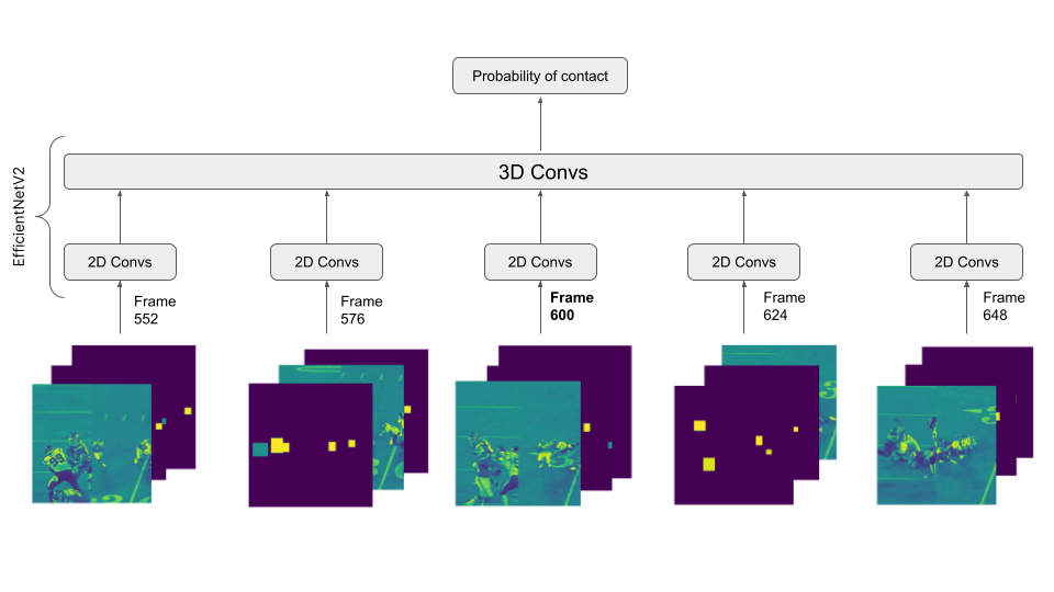\n\n\nWe will now explain in detail each of the channels. We have slight variations of these channels across models in our ensemble, but the core concept is the same. Please note that the order of channels is always the same, and the order is only changed for visual clarity in above architecture visualization, also only showing three channels, while our models use mostly five. Frames 552, 600 and 648 show the first channel in the foreground, while frame 576 shows the second frame, and 624 the fifth frame.\n\n**First channel**\nThe first channel depicts the region of interest of the potential contact only using the grayscale image. For each view, we take the center of the two (or one) boxes and then crop a total rectangle of width 128 and height 256. We then put both views next to each other resulting in a 256x256 input size. For most of our models we try to keep the aspect ratio based on box information and crop more information downwards than upwards to better capture the full body of players.\n\n**Second channel**\nHere we put a mask of the boxes to allow the model to clearly learn which players it should try to predict the contact for. We mask the two boxes with a value of 255. If there is only one box, or if there is a ground contact, we only mask this one box. We additionally mask all other boxes in this crop with 128.\n\n**Third channel**\nThe most important feature is the distance between two players. The CNN model itself can only learn the distance between players to some degree. So in this channel we directly decode the distance as derived from tracking information. Conveniently, there is a nice cutoff at around 2 yards where basically no contacts are present any longer. So we just multiply the distance by 128, giving us values between 0 and 255 that we encode in this channel.\n\n**Fourth channel**\nA very important feature was whether both players are from the same team. So here we just encode 255 if both are from the same team, and 128 otherwise.\n\n**Fifth channel**\nFinally, we saw that distance traveled of players from the last time point is helpful in tabular models. So similar to distance between players, we encode this feature separately for both players, or one in case of ground attack.\n\nFor all tracking feature channels, we stick to uint8 encoding which means we lose some precision for the features, but it helps with overfitting to it and can be seen as a binning between 256 bins similar to what GBM models do. The great benefit of encoding these features is that the CNNs can learn all the spatial and temporal information of such tracking features directly.\n\nAs the 2D backbone, we used `tf_efficientnetv2_s.in21k_ft_in1k` and `tf_efficientnetv2_b3` architecture and pre-trained weights from the timm library. We train all our models for 4 epochs and cosine schedule decay and AdamW optimizer. Checkpoints are always on last epoch.\n\n\n## Augmentations\nSpecifically mixup proved to be very useful in preventing quick overfitting. While it may appear counterintuitive to work well with the encoded feature channels, it likely acted as a good regularization. \nDuring training, we randomly shifted the image frame within a range of +-3 frames to the closest matching frame calculated from the current step. Furthermore, we used a small shift of +-1 for a subset of the model as test time augmentation in the ensemble. \n\n\n## Tracking and helmet interpolation\nFor the random frame shift augmentation, it was helpful to interpolate the tracking information from 10 Hz to 60 Hz. We tried a few different methods, but simple linear interpolation proved to be sufficient and is robust. We also added missing helmet box information using linear interpolation. While this definitely added some noise and false positives, overall it seemed to have helped catching a few more contacts in very crowded situations. We also use this interpolation for inference in our submissions.\n\n\n## Ensemble & Inference\nOur final ensemble consists of 6 models, and 3 seeds for each of them. All final models were retrained on the full data. We tried to add some diversity by different crop strategies and step sizes.\n\n\n|Backbone| Description | Step size | CV |\n| --- | --- | --- | --- |\n|tf_efficientnetv2_s.in21k_ft_in1k|No scaling of the crops|24|0.7899|\n|tf_efficientnetv2_b3|Slightly zoomed-in crops|24|0.7953|\n|tf_efficientnetv2_b3|Inverted feature channel encoding|24|0.7987|\n|tf_efficientnetv2_b3|No interpolation for boxes of other players|24|0.7989|\n|tf_efficientnetv2_b3|Inverted feature channel encoding|12 (4 times)|0.7988|\n|tf_efficientnetv2_s.in21k_ft_in1k|Smaller step size|6|0.7890| \n\n \n\n\nWe made full use of the recently added kernel with 2 T4 GPUs by parallelizing the pipeline and spawning two threads (1 CPU core for each to preprocess) each covering one half of the plays. All model predictions were averaged and subsequently fed to a stage 2 LGBM model. The final blend has a CV score of around 0.805 before the second stage.\n\n### Stage 2\nWe use a LGBM model with only a few carefully selected features including stage 1 ensemble probabilities, `nfl_player_id_1` to `nfl_player_id_2` distance and their lags. Other notable features are \"step_pct\", encoding the current step based on the play length and normalized X and Y positions on the field. Basically, using the average position of the two players and normalizing to one quarter of the field to prevent overfitting to single plays. \n\nIn the early stages of the competition, our 2nd stage model gave a great boost in score, specifically after adding the extra tracking features, while in the end the stage 1 predictions were almost on-par, showcasing how the stage 1 CNNs already efficiently learn from the encoded tracking feature channels.\n\nFinally, we blend the LGB predictions with the smoothed raw predictions (window of 3) from the ensemble in a 50:50 ratio.\n\nOur final solution has a CV score of 0.807, a public LB of 0.796, and a private LB of 0.796, exhibiting strong consistency and generalizability.\n\nHuge shoutout to my teammates @philippsinger and @ybabakhin!", "votes": null }, { "id": "2167506", "postDate": "03/03/2023 14:31:11", "content": "congratulations and thanks for sharing the solution!
", "rawMarkdown": "congratulations and thanks for sharing the solution!", "votes": null }, { "id": "2167713", "postDate": "03/03/2023 17:04:52", "content": "Congrats. I appreciate the clear write-up.
", "rawMarkdown": "Congrats. I appreciate the clear write-up.", "votes": null }, { "id": "2167744", "postDate": "03/03/2023 17:26:05", "content": "V interesting
", "rawMarkdown": "V interesting", "votes": null }, { "id": "2167959", "postDate": "03/03/2023 19:20:03", "content": "Great writeup @ilu000 and team (@philippsinger, @ybabakhin). This is a really elegant solution, congrats on the strong finish.
\nJust a few quick questions that come to mind after reading:
\nIt's interesting that interpolating the NGS data to 60Hz was beneficial, and was a smart idea to interpolate the helmet boxes. Also interesting that mixup augmentation helped.
\nThanks again for sharing! Looking forward to discussing more.
", "rawMarkdown": "Great writeup @ilu000 and team (@philippsinger, @ybabakhin). This is a really elegant solution, congrats on the strong finish.\n\nJust a few quick questions that come to mind after reading:\n\n- I'm trying to understand how the encoding of NGS features worked when you added them to channels 3-5. For these channels all values in the 256x256 image were the same - or did you only apply them to the helmet box areas?\n- Did you experiment at all with modeling player-to-ground separately than player-to-player? I'm surprised a single model was best because of how different these types of contact look visually.\n- How did you handle cases where players were not in view in both or either cameras? Did you only predict when both players could be seen and identified in the video? Did you account for those pairs in the stage 2 model?\n- Did you filter out player pairs with high separation distance before training/evaluation?\n- Am I reading it correctly that your stage 2 model improved the predictions from 0.805 -> 0.807 in your final CV?\n\nIt's interesting that interpolating the NGS data to 60Hz was beneficial, and was a smart idea to interpolate the helmet boxes. Also interesting that mixup augmentation helped.\n\nThanks again for sharing! Looking forward to discussing more.", "votes": null }, { "id": "2169066", "postDate": "03/04/2023 18:54:31", "content": "Congratulations! Great job guys!
", "rawMarkdown": "Congratulations! Great job guys!", "votes": null }, { "id": "2169124", "postDate": "03/04/2023 19:53:50", "content": "Thanks @robikscube !
\n\n\nI'm trying to understand how the encoding of NGS features worked when you added them to channels 3-5. For these channels all values in the 256x256 image were the same - or did you only apply them to the helmet box areas?
\n
We only applied them to the helmet box areas. But we also tried adding them to all pixels, and it did not really make a difference, as the model has the helmet channel anyways. It only makes a difference if both boxes exhibit different features, such as for distance travelled.
\n\n\nDid you experiment at all with modeling player-to-ground separately than player-to-player? I'm surprised a single model was best because of how different these types of contact look visually.
\n
We tried combined training and then finetuning separately, and it was not helpful. In general, such models can differentiate between these two types of contacts quite well, they can learn whether there is one box or two boxes marked, as well as how feature channels look like. We also checked the scores separately from time to time, and whenever we had a better model, both scores improved. Also blends and thresholds were super consistent across ground and player contacts. Maybe it is also one reason why our results are so stable, I would be curious if there are different number of ground and player contacts in public and private.
\n\n\nHow did you handle cases where players were not in view in both or either cameras? Did you only predict when both players could be seen and identified in the video? Did you account for those pairs in the stage 2 model?
\n
As we concatenate both views together, just having them in one view is not ideal, but not an issue, as the model can then just look at the other view. That's an advantage of the early fusion. Otherwise we did not handle it separately, if it cannot be seen at all we are feeding in an empty image. We tried a few things with the third view, but without success.
\n\n\nDid you filter out player pairs with high separation distance before training/evaluation?
\n
Yes, we filter out distance > 2, except for ground attacks, and set those predictions to zero.
\n\n\nAm I reading it correctly that your stage 2 model improved the predictions from 0.805 -> 0.807 in your final CV?
\n
Yes, it is only a tiny, but useful, boost in the end. It was very helpful early on, but the better we incorporated features into first stage, the more redundant it became. But for production one could absolutely consider ignoring it.
", "rawMarkdown": "Thanks @robikscube !\n\n> I'm trying to understand how the encoding of NGS features worked when you added them to channels 3-5. For these channels all values in the 256x256 image were the same - or did you only apply them to the helmet box areas?\n\nWe only applied them to the helmet box areas. But we also tried adding them to all pixels, and it did not really make a difference, as the model has the helmet channel anyways. It only makes a difference if both boxes exhibit different features, such as for distance travelled.\n\n> Did you experiment at all with modeling player-to-ground separately than player-to-player? I'm surprised a single model was best because of how different these types of contact look visually.\n\nWe tried combined training and then finetuning separately, and it was not helpful. In general, such models can differentiate between these two types of contacts quite well, they can learn whether there is one box or two boxes marked, as well as how feature channels look like. We also checked the scores separately from time to time, and whenever we had a better model, both scores improved. Also blends and thresholds were super consistent across ground and player contacts. Maybe it is also one reason why our results are so stable, I would be curious if there are different number of ground and player contacts in public and private.\n\n> How did you handle cases where players were not in view in both or either cameras? Did you only predict when both players could be seen and identified in the video? Did you account for those pairs in the stage 2 model?\n\nAs we concatenate both views together, just having them in one view is not ideal, but not an issue, as the model can then just look at the other view. That's an advantage of the early fusion. Otherwise we did not handle it separately, if it cannot be seen at all we are feeding in an empty image. We tried a few things with the third view, but without success.\n\n> Did you filter out player pairs with high separation distance before training/evaluation?\n\nYes, we filter out distance > 2, except for ground attacks, and set those predictions to zero. \n\n> Am I reading it correctly that your stage 2 model improved the predictions from 0.805 -> 0.807 in your final CV?\n\nYes, it is only a tiny, but useful, boost in the end. It was very helpful early on, but the better we incorporated features into first stage, the more redundant it became. But for production one could absolutely consider ignoring it.", "votes": null }, { "id": "2170426", "postDate": "03/06/2023 01:39:01", "content": "thankyou for your great sharing and well wirteup! I have a question. what is \"shift the image frame\" in the augmentation part?
", "rawMarkdown": "thankyou for your great sharing and well wirteup! I have a question. what is \"shift the image frame\" in the augmentation part?", "votes": null }, { "id": "2174171", "postDate": "03/08/2023 22:48:20", "content": "With \"shift the image frame\", we refer to an augmentation where we shift all input frames by X frames from the closest match that was calculated based on labels that were given in 10 Hz. We have video data in 60 Hz, so about 6 frames (±3 frames) can get the same label (nearest match from the given labels in 10 Hz).
", "rawMarkdown": "With \"shift the image frame\", we refer to an augmentation where we shift all input frames by X frames from the closest match that was calculated based on labels that were given in 10 Hz. We have video data in 60 Hz, so about 6 frames (±3 frames) can get the same label (nearest match from the given labels in 10 Hz).", "votes": null }, { "id": "2176544", "postDate": "03/10/2023 18:01:30", "content": "Excellent work and execution. Congrats!
", "rawMarkdown": "Excellent work and execution. Congrats!", "votes": null } ], "comments": [ { "id": 2167506, "author_name": "yuseokjung", "author_url": "", "post_date": "03/03/2023 14:31:11", "content": "congratulations and thanks for sharing the solution!
", "votes": null, "replies": [] }, { "id": 2167713, "author_name": "pcullen11", "author_url": "", "post_date": "03/03/2023 17:04:52", "content": "Congrats. I appreciate the clear write-up.
", "votes": null, "replies": [] }, { "id": 2167744, "author_name": "burn94", "author_url": "", "post_date": "03/03/2023 17:26:05", "content": "V interesting
", "votes": null, "replies": [] }, { "id": 2167959, "author_name": "robikscube", "author_url": "", "post_date": "03/03/2023 19:20:03", "content": "Great writeup @ilu000 and team (@philippsinger, @ybabakhin). This is a really elegant solution, congrats on the strong finish.
\nJust a few quick questions that come to mind after reading:
\nIt's interesting that interpolating the NGS data to 60Hz was beneficial, and was a smart idea to interpolate the helmet boxes. Also interesting that mixup augmentation helped.
\nThanks again for sharing! Looking forward to discussing more.
", "votes": null, "replies": [ { "id": 2169124, "author_name": "philippsinger", "author_url": "", "post_date": "03/04/2023 19:53:50", "content": "Thanks @robikscube !
\n\n\nI'm trying to understand how the encoding of NGS features worked when you added them to channels 3-5. For these channels all values in the 256x256 image were the same - or did you only apply them to the helmet box areas?
\n
We only applied them to the helmet box areas. But we also tried adding them to all pixels, and it did not really make a difference, as the model has the helmet channel anyways. It only makes a difference if both boxes exhibit different features, such as for distance travelled.
\n\n\nDid you experiment at all with modeling player-to-ground separately than player-to-player? I'm surprised a single model was best because of how different these types of contact look visually.
\n
We tried combined training and then finetuning separately, and it was not helpful. In general, such models can differentiate between these two types of contacts quite well, they can learn whether there is one box or two boxes marked, as well as how feature channels look like. We also checked the scores separately from time to time, and whenever we had a better model, both scores improved. Also blends and thresholds were super consistent across ground and player contacts. Maybe it is also one reason why our results are so stable, I would be curious if there are different number of ground and player contacts in public and private.
\n\n\nHow did you handle cases where players were not in view in both or either cameras? Did you only predict when both players could be seen and identified in the video? Did you account for those pairs in the stage 2 model?
\n
As we concatenate both views together, just having them in one view is not ideal, but not an issue, as the model can then just look at the other view. That's an advantage of the early fusion. Otherwise we did not handle it separately, if it cannot be seen at all we are feeding in an empty image. We tried a few things with the third view, but without success.
\n\n\nDid you filter out player pairs with high separation distance before training/evaluation?
\n
Yes, we filter out distance > 2, except for ground attacks, and set those predictions to zero.
\n\n\nAm I reading it correctly that your stage 2 model improved the predictions from 0.805 -> 0.807 in your final CV?
\n
Yes, it is only a tiny, but useful, boost in the end. It was very helpful early on, but the better we incorporated features into first stage, the more redundant it became. But for production one could absolutely consider ignoring it.
", "votes": null, "replies": [] } ] }, { "id": 2169066, "author_name": "cdeotte", "author_url": "", "post_date": "03/04/2023 18:54:31", "content": "Congratulations! Great job guys!
", "votes": null, "replies": [] }, { "id": 2170426, "author_name": "chg0901", "author_url": "", "post_date": "03/06/2023 01:39:01", "content": "thankyou for your great sharing and well wirteup! I have a question. what is \"shift the image frame\" in the augmentation part?
", "votes": null, "replies": [ { "id": 2174171, "author_name": "ilu000", "author_url": "", "post_date": "03/08/2023 22:48:20", "content": "With \"shift the image frame\", we refer to an augmentation where we shift all input frames by X frames from the closest match that was calculated based on labels that were given in 10 Hz. We have video data in 60 Hz, so about 6 frames (±3 frames) can get the same label (nearest match from the given labels in 10 Hz).
", "votes": null, "replies": [] } ] }, { "id": 2176544, "author_name": "tariqbashir", "author_url": "", "post_date": "03/10/2023 18:01:30", "content": "Excellent work and execution. Congrats!
", "votes": null, "replies": [] } ], "raw_markdown_by_id": { "2165886": "Thank you for another great NFL challenge! As the previous NFL competitions it was well prepared and had quick feedback cycles anytime that the community had questions. We would like to highlight @robikscube, one of the hosts, who even supplied a strong tabular baseline to get started. \n\n## Validation\nThe test data is rather small compared to the large training set and only consists of 61 plays. Thus, local validation becomes even more important than usual. To evaluate our models, we used Stratified Group KFold cross validation on the `game_key` and public LB usually followed any local CV improvements with only a small random range of a few points and with blends being a bit more stable than single models (5 folds or a handful of fullfits). Our best local CV was 0.807 for the blend including 2nd stage and about 0.802 for a single model including 2nd stage. \n\n## Models and architecture\nThe core ideas and central building blocks of our models are based on our concepts of the previous DFL competition (https://www.kaggle.com/competitions/dfl-bundesliga-data-shootout/discussion/359932) utilizing 2D/3D CNNs capturing temporal aspects of videos. This architecture has already served us well in multiple video sports projects and competitions and also turned out to be highly competitive here.\n\nIn this competition we found longer time steps to work better and we got our best single model results using a time step of 24 frames, two times in both directions. We crop the region of interest for each potential contact based on helmet box information. In most models, we resize the crop, so that all boxes have about the same size. We concatenate endzone and sideline views horizontally to enable early fusion. Additionally, we encode tracking data directly into the CNN models. This has the main advantage that we can mostly rely on a single stage solution, and are less prone to overfitting on a 2-stage approach with out-of-fold CNN predictions. We step-wise encoded tracking features based on their importance in tabular models.\n\nThe main architecture of our approach looks like the following:\n\n\n\n\nWe will now explain in detail each of the channels. We have slight variations of these channels across models in our ensemble, but the core concept is the same. Please note that the order of channels is always the same, and the order is only changed for visual clarity in above architecture visualization, also only showing three channels, while our models use mostly five. Frames 552, 600 and 648 show the first channel in the foreground, while frame 576 shows the second frame, and 624 the fifth frame.\n\n**First channel**\nThe first channel depicts the region of interest of the potential contact only using the grayscale image. For each view, we take the center of the two (or one) boxes and then crop a total rectangle of width 128 and height 256. We then put both views next to each other resulting in a 256x256 input size. For most of our models we try to keep the aspect ratio based on box information and crop more information downwards than upwards to better capture the full body of players.\n\n**Second channel**\nHere we put a mask of the boxes to allow the model to clearly learn which players it should try to predict the contact for. We mask the two boxes with a value of 255. If there is only one box, or if there is a ground contact, we only mask this one box. We additionally mask all other boxes in this crop with 128.\n\n**Third channel**\nThe most important feature is the distance between two players. The CNN model itself can only learn the distance between players to some degree. So in this channel we directly decode the distance as derived from tracking information. Conveniently, there is a nice cutoff at around 2 yards where basically no contacts are present any longer. So we just multiply the distance by 128, giving us values between 0 and 255 that we encode in this channel.\n\n**Fourth channel**\nA very important feature was whether both players are from the same team. So here we just encode 255 if both are from the same team, and 128 otherwise.\n\n**Fifth channel**\nFinally, we saw that distance traveled of players from the last time point is helpful in tabular models. So similar to distance between players, we encode this feature separately for both players, or one in case of ground attack.\n\nFor all tracking feature channels, we stick to uint8 encoding which means we lose some precision for the features, but it helps with overfitting to it and can be seen as a binning between 256 bins similar to what GBM models do. The great benefit of encoding these features is that the CNNs can learn all the spatial and temporal information of such tracking features directly.\n\nAs the 2D backbone, we used `tf_efficientnetv2_s.in21k_ft_in1k` and `tf_efficientnetv2_b3` architecture and pre-trained weights from the timm library. We train all our models for 4 epochs and cosine schedule decay and AdamW optimizer. Checkpoints are always on last epoch.\n\n\n## Augmentations\nSpecifically mixup proved to be very useful in preventing quick overfitting. While it may appear counterintuitive to work well with the encoded feature channels, it likely acted as a good regularization. \nDuring training, we randomly shifted the image frame within a range of +-3 frames to the closest matching frame calculated from the current step. Furthermore, we used a small shift of +-1 for a subset of the model as test time augmentation in the ensemble. \n\n\n## Tracking and helmet interpolation\nFor the random frame shift augmentation, it was helpful to interpolate the tracking information from 10 Hz to 60 Hz. We tried a few different methods, but simple linear interpolation proved to be sufficient and is robust. We also added missing helmet box information using linear interpolation. While this definitely added some noise and false positives, overall it seemed to have helped catching a few more contacts in very crowded situations. We also use this interpolation for inference in our submissions.\n\n\n## Ensemble & Inference\nOur final ensemble consists of 6 models, and 3 seeds for each of them. All final models were retrained on the full data. We tried to add some diversity by different crop strategies and step sizes.\n\n\n|Backbone| Description | Step size | CV |\n| --- | --- | --- | --- |\n|tf_efficientnetv2_s.in21k_ft_in1k|No scaling of the crops|24|0.7899|\n|tf_efficientnetv2_b3|Slightly zoomed-in crops|24|0.7953|\n|tf_efficientnetv2_b3|Inverted feature channel encoding|24|0.7987|\n|tf_efficientnetv2_b3|No interpolation for boxes of other players|24|0.7989|\n|tf_efficientnetv2_b3|Inverted feature channel encoding|12 (4 times)|0.7988|\n|tf_efficientnetv2_s.in21k_ft_in1k|Smaller step size|6|0.7890| \n\n \n\n\nWe made full use of the recently added kernel with 2 T4 GPUs by parallelizing the pipeline and spawning two threads (1 CPU core for each to preprocess) each covering one half of the plays. All model predictions were averaged and subsequently fed to a stage 2 LGBM model. The final blend has a CV score of around 0.805 before the second stage.\n\n### Stage 2\nWe use a LGBM model with only a few carefully selected features including stage 1 ensemble probabilities, `nfl_player_id_1` to `nfl_player_id_2` distance and their lags. Other notable features are \"step_pct\", encoding the current step based on the play length and normalized X and Y positions on the field. Basically, using the average position of the two players and normalizing to one quarter of the field to prevent overfitting to single plays. \n\nIn the early stages of the competition, our 2nd stage model gave a great boost in score, specifically after adding the extra tracking features, while in the end the stage 1 predictions were almost on-par, showcasing how the stage 1 CNNs already efficiently learn from the encoded tracking feature channels.\n\nFinally, we blend the LGB predictions with the smoothed raw predictions (window of 3) from the ensemble in a 50:50 ratio.\n\nOur final solution has a CV score of 0.807, a public LB of 0.796, and a private LB of 0.796, exhibiting strong consistency and generalizability.\n\nHuge shoutout to my teammates @philippsinger and @ybabakhin!", "2167506": "congratulations and thanks for sharing the solution!", "2167713": "Congrats. I appreciate the clear write-up.", "2167744": "V interesting", "2167959": "Great writeup @ilu000 and team (@philippsinger, @ybabakhin). This is a really elegant solution, congrats on the strong finish.\n\nJust a few quick questions that come to mind after reading:\n\n- I'm trying to understand how the encoding of NGS features worked when you added them to channels 3-5. For these channels all values in the 256x256 image were the same - or did you only apply them to the helmet box areas?\n- Did you experiment at all with modeling player-to-ground separately than player-to-player? I'm surprised a single model was best because of how different these types of contact look visually.\n- How did you handle cases where players were not in view in both or either cameras? Did you only predict when both players could be seen and identified in the video? Did you account for those pairs in the stage 2 model?\n- Did you filter out player pairs with high separation distance before training/evaluation?\n- Am I reading it correctly that your stage 2 model improved the predictions from 0.805 -> 0.807 in your final CV?\n\nIt's interesting that interpolating the NGS data to 60Hz was beneficial, and was a smart idea to interpolate the helmet boxes. Also interesting that mixup augmentation helped.\n\nThanks again for sharing! Looking forward to discussing more.", "2169066": "Congratulations! Great job guys!", "2169124": "Thanks @robikscube !\n\n> I'm trying to understand how the encoding of NGS features worked when you added them to channels 3-5. For these channels all values in the 256x256 image were the same - or did you only apply them to the helmet box areas?\n\nWe only applied them to the helmet box areas. But we also tried adding them to all pixels, and it did not really make a difference, as the model has the helmet channel anyways. It only makes a difference if both boxes exhibit different features, such as for distance travelled.\n\n> Did you experiment at all with modeling player-to-ground separately than player-to-player? I'm surprised a single model was best because of how different these types of contact look visually.\n\nWe tried combined training and then finetuning separately, and it was not helpful. In general, such models can differentiate between these two types of contacts quite well, they can learn whether there is one box or two boxes marked, as well as how feature channels look like. We also checked the scores separately from time to time, and whenever we had a better model, both scores improved. Also blends and thresholds were super consistent across ground and player contacts. Maybe it is also one reason why our results are so stable, I would be curious if there are different number of ground and player contacts in public and private.\n\n> How did you handle cases where players were not in view in both or either cameras? Did you only predict when both players could be seen and identified in the video? Did you account for those pairs in the stage 2 model?\n\nAs we concatenate both views together, just having them in one view is not ideal, but not an issue, as the model can then just look at the other view. That's an advantage of the early fusion. Otherwise we did not handle it separately, if it cannot be seen at all we are feeding in an empty image. We tried a few things with the third view, but without success.\n\n> Did you filter out player pairs with high separation distance before training/evaluation?\n\nYes, we filter out distance > 2, except for ground attacks, and set those predictions to zero. \n\n> Am I reading it correctly that your stage 2 model improved the predictions from 0.805 -> 0.807 in your final CV?\n\nYes, it is only a tiny, but useful, boost in the end. It was very helpful early on, but the better we incorporated features into first stage, the more redundant it became. But for production one could absolutely consider ignoring it.", "2170426": "thankyou for your great sharing and well wirteup! I have a question. what is \"shift the image frame\" in the augmentation part?", "2174171": "With \"shift the image frame\", we refer to an augmentation where we shift all input frames by X frames from the closest match that was calculated based on labels that were given in 10 Hz. We have video data in 60 Hz, so about 6 frames (±3 frames) can get the same label (nearest match from the given labels in 10 Hz).", "2176544": "Excellent work and execution. Congrats!" }, "source": "meta" }