{"cells":[{"metadata":{},"cell_type":"markdown","source":"","execution_count":null},{"metadata":{},"cell_type":"markdown","source":"\nContents\n* [Threat in using augmented Data]()\n* [Tackle with label smoothing]()\n* [Expirement with label smoothing]()\n\n","execution_count":null},{"metadata":{},"cell_type":"markdown","source":"## Please leave an upvote if you like this Notebook\n","execution_count":null},{"metadata":{},"cell_type":"markdown","source":"In this competition we are trying to use many data augmentation methods, especially to generate more data on languages other than English and train on those examples.\n\nThe methods used until now are :\n- [Translating data using Google API](https://www.kaggle.com/c/jigsaw-multilingual-toxic-comment-classification/discussion/141377)\n- [NLP Albumentation](https://www.kaggle.com/shonenkov/nlp-albumentations)\n- [Parellel corpus](https://www.kaggle.com/shonenkov/hack-with-parallel-corpus)\n\nI went through all of these methods and tried some of the them.No doubt, they are pretty useful. But after reading the recent notebook from [Alex Shonenkov](https://www.kaggle.com/shonenkov) I got a link to the idea of label smoothing which I am going to discuss here.All these data augmentation methods have a possible hidden threat in them which is why many of us are still in a dilemma whether to use them or not.\n\nThe main possible threat is that there is a chance that these methods produce data samples with incorrect labels.I tried using Google translate API to some of the toxic comments and I saw that sometimes it is censoring the toxic content in some comments or reducing the level of toxicity in it( I saw it happen using google API). This can happen to other augmentation methods too...\n\nSo, what's the solution to this problem?\n- Don't bother to use the augmentation methods and lose the edge that it gives.\n- Use Label Smoothing.\n\n**So let's do label smoothing.**","execution_count":null},{"metadata":{},"cell_type":"markdown","source":"## Say hello to Label Smoothing!\n\nWhen we apply the cross-entropy loss to a classification task, we’re expecting true labels to have 1, while the others 0. In other words, we have no doubts that the true labels are true, and the others are not. Is that always true in our case? As said above, the translation or other augmentation methods have done some mistakes. They might have different criteria. They might make some mistakes. As a result, the ground truth labels we have had perfect beliefs on are possibly wrong. In our case, a sample with no toxicity will have had perfect belief as toxic or vice versa...\n\nOne possible solution to this is to relax our confidence on the labels. For instance, we can slightly lower the loss target values from 1 to, say, 0.9. And naturally, we increase the target value of 0 for the others slightly as such. This idea is called label smoothing.\n\n[](https://postimg.cc/VrcnKqsZ)\nIn tensorflow,","execution_count":null},{"metadata":{"_kg_hide-output":true,"trusted":true},"cell_type":"code","source":"import tensorflow as tf\n\ntf.keras.losses.binary_crossentropy(\n y_true, y_pred,\n from_logits=False,\n label_smoothing=0\n)\n","execution_count":null,"outputs":[]},{"metadata":{},"cell_type":"markdown","source":"If label_smoothing is nonzero, smooth the labels towards 1/num_classes:\n\n\n`new_onehot_labels = onehot_labels * (1 – label_smoothing) + label_smoothing / num_classes`\n\nWhat does this mean?\n\nWell, say in our case were training a model for binary classification,Our labels are 0 — Non-toxic, 1 — toxic.\n\nNow, say you label_smoothing = 0.2\n\nUsing the equation above, we get:\n\n`new_labels = [0 1] * (1 — 0.2) + 0.2 / 2 =[0 1]*(0.8) + 0.1`\n\n `new_labels = [0.1 ,0.9]`\n","execution_count":null},{"metadata":{},"cell_type":"markdown","source":"OR you can simply convert your one hot encoded array of floating point numbers to the “nuanced” version\n","execution_count":null},{"metadata":{"_kg_hide-output":true,"trusted":true},"cell_type":"code","source":"\ntrain[np.where(y == 0)] = 0.1\ntrain[np.where(y == 1)] = 0.9\n","execution_count":null,"outputs":[]},{"metadata":{},"cell_type":"markdown","source":"## What does this do ?","execution_count":null},{"metadata":{},"cell_type":"markdown","source":"One should see the values 0 and 1 as simply true and false. Taking values that vary slightly from the classic values, they are a more nuanced way to describing the data 0.1 could be viewed as: “there is a very low chance this data is ” whereas 0.9\n\nis, of course, a high chance.\n\nUsing these “nuanced” labels, the cost of an incorrect prediction is slightly lower than using “hard” labels resulting in a smaller gradient. While this intuition helped me understand why it could be a good idea, I was not entirely convinced it would work in an application because the loss is lowered for all wrong classifications. So I decided to read some about some research done on the subject.\n\nA table copied from [When Does Label Smoothing Help?](https://arxiv.org/pdf/1906.02629.pdf)\n\n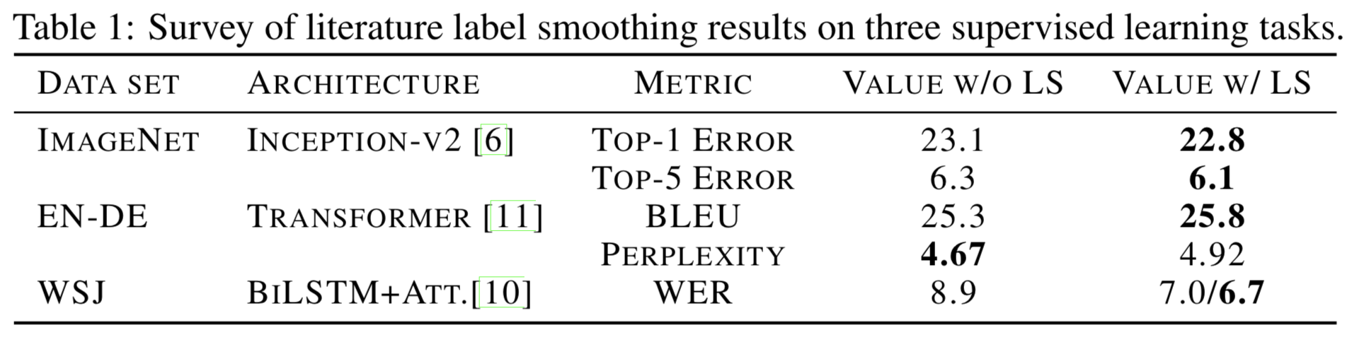","execution_count":null},{"metadata":{},"cell_type":"markdown","source":"## Expirement with Label Smoothing","execution_count":null},{"metadata":{},"cell_type":"markdown","source":"Now,it's time to expirement with the same.For the sake our expirement I will take the data from `sklearn.datasets`. We need a binary classificatin example,so I selected `breast cancer` dataset which contains approx 500 samples with 30 features.","execution_count":null},{"metadata":{"trusted":true},"cell_type":"code","source":"","execution_count":null,"outputs":[]},{"metadata":{"trusted":true},"cell_type":"code","source":"from sklearn.datasets import load_breast_cancer\nfrom sklearn.model_selection import train_test_split\nfrom sklearn.metrics import accuracy_score\nimport matplotlib.pyplot as plt\nimport tensorflow as tf\nimport numpy as np\nplt.style.use('ggplot')\nepochs=10","execution_count":null,"outputs":[]},{"metadata":{},"cell_type":"markdown","source":"Let's load the dataset and see","execution_count":null},{"metadata":{"trusted":true},"cell_type":"code","source":"data= load_breast_cancer()","execution_count":null,"outputs":[]},{"metadata":{"trusted":true},"cell_type":"code","source":"print(\"The dataset contains {} samples with {} features\".format(data['data'].shape[0],data['data'].shape[1]))\n","execution_count":null,"outputs":[]},{"metadata":{},"cell_type":"markdown","source":"- Let's do the train and test split now,(80:20)","execution_count":null},{"metadata":{"trusted":true},"cell_type":"code","source":"train_X,test_X,train_y,test_y=train_test_split(data['data'],data['target'],random_state=77)","execution_count":null,"outputs":[]},{"metadata":{},"cell_type":"markdown","source":"Now for our expirement I will relabel some of the negative cases (target 0 ) as positive cases (target 1).","execution_count":null},{"metadata":{"trusted":true},"cell_type":"code","source":"train_y[:40]=1","execution_count":null,"outputs":[]},{"metadata":{},"cell_type":"markdown","source":"Next,let's build our simple NN model","execution_count":null},{"metadata":{"trusted":true},"cell_type":"code","source":"def model():\n inp = tf.keras.Input(shape=(30))\n \n x= tf.keras.layers.Dense(64,activation='relu')(inp)\n x=tf.keras.layers.Dense(32,activation='relu')(x)\n x=tf.keras.layers.Dense(1,'sigmoid')(x)\n \n model=tf.keras.Model(inp,x)\n model.compile(optimizer='Adam',loss='binary_crossentropy',metrics=['accuracy'])\n return model\n \n ","execution_count":null,"outputs":[]},{"metadata":{"trusted":true},"cell_type":"code","source":"model=model()\nmodel.summary()","execution_count":null,"outputs":[]},{"metadata":{},"cell_type":"markdown","source":"Now, Fit ,evaluate and predict **without label smoothing**","execution_count":null},{"metadata":{"trusted":true},"cell_type":"code","source":"\nhistory=model.fit(train_X,train_y,epochs=epochs)","execution_count":null,"outputs":[]},{"metadata":{},"cell_type":"markdown","source":"","execution_count":null},{"metadata":{"trusted":true},"cell_type":"code","source":"plt.figure(figsize=(10,5))\nplt.subplot(1,2,1)\nplt.plot(np.arange(1,epochs+1),history.history['loss'],color='red',alpha=1)\nplt.gca().set_xlabel(\"Epochs\")\nplt.gca().set_ylabel(\"loss\")\nplt.gca().set_title(\"Loss without Label smoothing\")\n\nplt.subplot(1,2,2)\nplt.plot(np.arange(1,epochs+1),history.history['accuracy'],color='red',alpha=1)\nplt.gca().set_xlabel(\"Epochs\")\nplt.gca().set_ylabel(\"accuracy\")\nplt.gca().set_title(\"accuracy without Label smoothing\")\n\n\nplt.show()","execution_count":null,"outputs":[]},{"metadata":{"trusted":true},"cell_type":"code","source":"y_pre = model.predict(test_X)\nprint(accuracy_score(test_y,np.round(y_pre)))","execution_count":null,"outputs":[]},{"metadata":{},"cell_type":"markdown","source":"You can see that the model has an accuracy of only 67% in the test set.\n- Now let's add the trick and train our model.Train our model **with label smoothing**","execution_count":null},{"metadata":{"trusted":true},"cell_type":"code","source":"def label_smoothing(y_true,y_pred):\n \n return tf.keras.losses.binary_crossentropy(y_true,y_pred,label_smoothing=0.1)","execution_count":null,"outputs":[]},{"metadata":{"trusted":true},"cell_type":"code","source":"def model():\n inp = tf.keras.Input(shape=(30))\n \n x= tf.keras.layers.Dense(64,activation='relu')(inp)\n x=tf.keras.layers.Dense(32,activation='relu')(x)\n x=tf.keras.layers.Dense(1,'sigmoid')(x)\n \n model=tf.keras.Model(inp,x)\n \n model.compile(optimizer='Adam',loss=label_smoothing,metrics=['accuracy'])\n return model\n ","execution_count":null,"outputs":[]},{"metadata":{"trusted":true},"cell_type":"code","source":"model=model()\nhistory=model.fit(train_X,train_y,epochs=epochs)","execution_count":null,"outputs":[]},{"metadata":{"trusted":true},"cell_type":"code","source":"plt.figure(figsize=(10,5))\nplt.subplot(1,2,1)\nplt.plot(np.arange(1,epochs+1),history.history['loss'],color='red',alpha=1)\nplt.gca().set_xlabel(\"Epochs\")\nplt.gca().set_ylabel(\"loss\")\nplt.gca().set_title(\"Loss with Label smoothing\")\n\nplt.subplot(1,2,2)\nplt.plot(np.arange(1,epochs+1),history.history['accuracy'],color='red',alpha=1)\nplt.gca().set_xlabel(\"Epochs\")\nplt.gca().set_ylabel(\"accuracy\")\nplt.gca().set_title(\"accuracy with Label smoothing\")\n\n\nplt.show()","execution_count":null,"outputs":[]},{"metadata":{},"cell_type":"markdown","source":"Now,the moment of truth !\n- let's predict on the same test set and see how much accuracy does it give...","execution_count":null},{"metadata":{"trusted":true},"cell_type":"code","source":"y_pre = model.predict(test_X)\nprint(accuracy_score(test_y,np.round(y_pre)))","execution_count":null,"outputs":[]},{"metadata":{},"cell_type":"markdown","source":"viola..! The accuracy just increased just by adding **label smoothing**.","execution_count":null},{"metadata":{},"cell_type":"markdown","source":"I hope this helps,I encourage you to try this and comment your results below.\n## Please leave an upvote if you like this Notebook\n\nReferences :\n- https://arxiv.org/pdf/1906.02629.pdf\n- https://www.flixstock.com/label-smoothing-an-ingredient-of-higher-model-accuracy/","execution_count":null}],"metadata":{"kernelspec":{"language":"python","display_name":"Python 3","name":"python3"},"language_info":{"pygments_lexer":"ipython3","nbconvert_exporter":"python","version":"3.6.4","file_extension":".py","codemirror_mode":{"name":"ipython","version":3},"name":"python","mimetype":"text/x-python"}},"nbformat":4,"nbformat_minor":4}