{"metadata":{"kernelspec":{"name":"python3","display_name":"Python 3","language":"python"},"language_info":{"name":"python","version":"3.11.11","mimetype":"text/x-python","codemirror_mode":{"name":"ipython","version":3},"pygments_lexer":"ipython3","nbconvert_exporter":"python","file_extension":".py"},"colab":{"provenance":[]},"kaggle":{"accelerator":"nvidiaTeslaT4","dataSources":[{"sourceId":6799,"databundleVersionId":4225553,"isSourceIdPinned":false,"sourceType":"competition"},{"sourceId":11735731,"sourceType":"datasetVersion","datasetId":7367395}],"dockerImageVersionId":31011,"isInternetEnabled":true,"language":"python","sourceType":"notebook","isGpuEnabled":true}},"nbformat_minor":4,"nbformat":4,"cells":[{"cell_type":"code","source":"name = \"AlirezaEbrahimzadeh\"\nstudent_id = \"402204244\"\n\n\n### Note : THis code should be run on kaggle (last about 1H)\n### Note : Before run , u have to add ILSVRC dataset to ur input dataset , (https://www.kaggle.com/c/imagenet-object-localization-challenge/overview/description)\n### for add dataset Type \"imagenet object localization challenge\"","metadata":{"id":"HGLz4ym6_GkH","outputId":"bdd7418a-bd8a-438c-ed32-6c87d3392b7b","trusted":true,"execution":{"iopub.status.busy":"2025-05-09T19:14:27.69048Z","iopub.execute_input":"2025-05-09T19:14:27.691195Z","iopub.status.idle":"2025-05-09T19:14:27.694526Z","shell.execute_reply.started":"2025-05-09T19:14:27.69117Z","shell.execute_reply":"2025-05-09T19:14:27.693802Z"}},"outputs":[],"execution_count":null},{"cell_type":"markdown","source":"# 1.Adversarial attacks","metadata":{"id":"Y4-piPsWenfI"}},{"cell_type":"markdown","source":"In this homework, we will discuss adversarial attacks on deep image classification models. Deep Neural Networks are a very powerful tool to recognize patterns in data, and, for example, perform image classification on a human-level. However, we have not tested yet how robust these models actually are. Can we \"trick\" the model and find failure modes? Can we design images that the networks naturally classify incorrectly? Due to the high classification accuracy on unseen test data, we would expect that this can be difficult. However, in 2014, a research group at Google and NYU showed that deep CNNs can be easily fooled, just by adding some salient but carefully constructed noise to the images. For instance, take a look at the example below (figure credit - [Goodfellow et al.](https://arxiv.org/pdf/1412.6572.pdf)):\n\n)\n object_elem = root.find(\"object\")\n if object_elem is not None:\n class_name = object_elem.find(\"name\").text\n class_to_images[class_name].append(filename)\n\n# Create output directory\nos.makedirs(OUTPUT_DIR_VAL, exist_ok=True)\n\nfor class_name, image_list in class_to_images.items():\n output_class_dir = os.path.join(OUTPUT_DIR_VAL, class_name)\n os.makedirs(output_class_dir, exist_ok=True)\n\n for img_name in sorted(image_list)[:]:\n src_img_path = os.path.join(VAL_IMAGES_DIR, img_name+\".JPEG\")\n dst_img_path = os.path.join(output_class_dir, img_name+\".JPEG\")\n shutil.copy(src_img_path, dst_img_path)\n\n","metadata":{"trusted":true,"execution":{"iopub.status.busy":"2025-05-09T17:53:08.652989Z","iopub.execute_input":"2025-05-09T17:53:08.653331Z","iopub.status.idle":"2025-05-09T18:09:30.26056Z","shell.execute_reply.started":"2025-05-09T17:53:08.653313Z","shell.execute_reply":"2025-05-09T18:09:30.259907Z"}},"outputs":[],"execution_count":null},{"cell_type":"markdown","source":"## Deep CNNs on ImageNet\n\nFor our experiments in this notebook, we will use common CNN architectures trained on the ImageNet dataset. Such models are luckily provided by PyTorch's torchvision package, and hence we just need to load the model of our preference. For the results default on Google Colab, we use a ResNet34.","metadata":{"id":"iwfzY8L7enfL"}},{"cell_type":"markdown","source":"# 5 Points","metadata":{"id":"-hGRwFqP6BVu"}},{"cell_type":"code","source":"from torchvision import models\n\n\npretrained_model = models.resnet34(pretrained=True)\n\n# no gradiant\nfor param in pretrained_model.parameters():\n param.requires_grad = False\n\n\nfor param in pretrained_model.fc.parameters():\n param.requires_grad = True\n\n# Move to GPu\npretrained_model = pretrained_model.to(device)\n\nprint(pretrained_model)\n","metadata":{"id":"U4niSCpIenfL","trusted":true,"execution":{"iopub.status.busy":"2025-05-09T18:09:30.267473Z","iopub.execute_input":"2025-05-09T18:09:30.267685Z","iopub.status.idle":"2025-05-09T18:09:31.902599Z","shell.execute_reply.started":"2025-05-09T18:09:30.267668Z","shell.execute_reply":"2025-05-09T18:09:31.901902Z"}},"outputs":[],"execution_count":null},{"cell_type":"markdown","source":"To perform adversarial attacks, we also need a dataset to work on. Given that the CNN model has been trained on ImageNet, it is only fair to perform the attacks on data from ImageNet. For this, we provide a small set of pre-processed images from the original ImageNet dataset . Specifically, we have 5 images for each of the 1000 labels of the dataset. We can load the data below, and create a corresponding data loader.","metadata":{"id":"LbJberveenfM"}},{"cell_type":"markdown","source":"# 5 Points","metadata":{"id":"gchd0S5t6DRX"}},{"cell_type":"code","source":"#resize tensor to uniform size\n\ntransform = transforms.Compose([\n transforms.Resize((256, 256)),\n transforms.ToTensor()\n])\n\n#create dataset and dataloader\ndataset = torchvision.datasets.ImageFolder(OUTPUT_DIR_VAL,transform=transform)\ndataloader = data.DataLoader(dataset, batch_size=128, shuffle=True, num_workers=4)\n\n#calculate mean and std\nmean = 0.0\nstd = 0.0\nnb_samples = 0\n\nfor data, _ in dataloader:\n batch_samples = data.size(0)\n data = data.view(batch_samples, data.size(1), -1) # flatten H and W\n mean += data.mean(2).sum(0)\n std += data.std(2).sum(0)\n nb_samples += batch_samples\n\nmean /= nb_samples\nstd /= nb_samples\n\n\n\nprint(\"Mean:\", mean)\nprint(\"Std:\", std)","metadata":{"trusted":true,"execution":{"iopub.status.busy":"2025-05-09T18:09:31.903356Z","iopub.execute_input":"2025-05-09T18:09:31.903572Z","iopub.status.idle":"2025-05-09T18:12:06.222104Z","shell.execute_reply.started":"2025-05-09T18:09:31.903555Z","shell.execute_reply":"2025-05-09T18:12:06.221283Z"}},"outputs":[],"execution_count":null},{"cell_type":"code","source":"import torch.utils.data as data\n\n\nfile_path = '/kaggle/input/imagenet-object-localization-challenge/LOC_synset_mapping.txt'\nwith open(file_path, 'r') as file:\n file_content = file.read()\n\n#create dic of labels dic\n\nlabel_images = {}\nfor idx, line in enumerate(file_content.strip().split(\"\\n\")):\n parts = line.split()\n wnid = parts[0] # WordNet ID\n labels = \" \".join(parts[1:]).split(\", \") # Split labels\n label_images[idx] = [wnid] + labels\n\nfor key in label_images:\n label_images[key] = label_images[key][1:]\n\n\n\ntransform = transforms.Compose([\n transforms.Resize((256, 256)),\n transforms.ToTensor(),\n transforms.Normalize(mean=mean, std=std)\n])\nos.makedirs(\"/kaggle/working/val_subset\", exist_ok=True)\n\n\nN_IMAGES = 5\n\n\nfor class_name in sorted(os.listdir(\"/kaggle/working/val\")):\n class_input_path = os.path.join(\"/kaggle/working/val\", class_name)\n class_output_path = os.path.join(\"/kaggle/working/val_subset\", class_name)\n\n os.makedirs(class_output_path, exist_ok=True)\n\n image_files = [f for f in os.listdir(class_input_path) if f.lower().endswith(('.jpg', '.jpeg', '.png'))]\n\n for img_file in sorted(image_files)[:N_IMAGES]:\n src = os.path.join(class_input_path, img_file)\n dst = os.path.join(class_output_path, img_file)\n shutil.copy(src, dst)\n# create sub dataloader that have 5 pics of each 1000 classes\nsub_dataset = torchvision.datasets.ImageFolder(\"/kaggle/working/val_subset\", transform=transform)\nsub_dataloader = data.DataLoader(sub_dataset, batch_size=128, shuffle=True, num_workers=4)","metadata":{"id":"SQvHwe4zenfM","trusted":true,"execution":{"iopub.status.busy":"2025-05-09T18:12:06.223166Z","iopub.execute_input":"2025-05-09T18:12:06.223462Z","iopub.status.idle":"2025-05-09T18:12:07.648515Z","shell.execute_reply.started":"2025-05-09T18:12:06.223437Z","shell.execute_reply":"2025-05-09T18:12:07.647939Z"}},"outputs":[],"execution_count":null},{"cell_type":"markdown","source":"Before we start with our attacks, we should verify the performance of our model. As ImageNet has 1000 classes, simply looking at the accuracy is not sufficient to tell the performance of a model. Imagine a model that always predicts the true label as the second-highest class in its softmax output. Although we would say it recognizes the object in the image, it achieves an accuracy of 0. In ImageNet with 1000 classes, there is not always one clear label we can assign an image to. This is why for image classifications over so many classes, a common alternative metric is \"Top-5 accuracy\", which tells us how many times the true label has been within the 5 most-likely predictions of the model. As models usually perform quite well on those, we report the error (1 - accuracy) instead of the accuracy:","metadata":{"id":"D1bOw3YIenfM"}},{"cell_type":"markdown","source":"# 10 Points","metadata":{"id":"0kKMSDWH6FaS"}},{"cell_type":"code","source":"#evaluate model\ndef eval_model(dataset_loader, img_func=None):\n model.eval()\n correct = 0\n top5_correct = 0\n total = 0\n\n with torch.no_grad():\n for imgs, labels in tqdm(dataset_loader, desc=\"Evaluating\", leave=False):\n imgs, labels = imgs.to(device), labels.to(device)\n\n output = model(imgs)\n _, preds = output.topk(5, dim=1)\n\n # Top-1 accuracy\n correct += (preds[:, 0] == labels).sum().item()\n # Top-5 accuracy\n top5_correct += sum([labels[i] in preds[i] for i in range(labels.size(0))])\n total += labels.size(0)\n\n acc = correct / total\n top5 = top5_correct / total\n\n print(f\"Top-1 error: {(1-acc)*100:.2f}%\")\n print(f\"Top-5 error: {(1-top5)*100:.2f}%\")\n return acc, top5\n","metadata":{"id":"rRbwtX9PenfM","trusted":true,"execution":{"iopub.status.busy":"2025-05-09T18:12:07.649506Z","iopub.execute_input":"2025-05-09T18:12:07.649721Z","iopub.status.idle":"2025-05-09T18:12:07.655477Z","shell.execute_reply.started":"2025-05-09T18:12:07.649704Z","shell.execute_reply":"2025-05-09T18:12:07.654894Z"}},"outputs":[],"execution_count":null},{"cell_type":"code","source":"model=pretrained_model\n_ = eval_model(sub_dataloader)","metadata":{"id":"S6nS1_H0enfN","outputId":"16b62239-3804-4469-d23a-21f9879d309e","trusted":true,"execution":{"iopub.status.busy":"2025-05-09T18:12:07.656133Z","iopub.execute_input":"2025-05-09T18:12:07.656384Z","iopub.status.idle":"2025-05-09T18:12:26.324831Z","shell.execute_reply.started":"2025-05-09T18:12:07.656367Z","shell.execute_reply":"2025-05-09T18:12:26.323282Z"}},"outputs":[],"execution_count":null},{"cell_type":"markdown","source":"The ResNet34 achives a decent error rate of 4.3% for the top-5 predictions. Next, we can look at some predictions of the model to get more familiar with the dataset. The function below plots an image along with a bar diagram of its predictions. We also prepare it to show adversarial examples for later applications.","metadata":{"id":"08AeGyoRenfN"}},{"cell_type":"markdown","source":"# 15 Points","metadata":{"id":"ggHoLMUQ6I6C"}},{"cell_type":"code","source":"def show_prediction(img, label, pred, K=5, adv_img=None, noise=None):\n\n img_np = img.cpu().permute(1, 2, 0).numpy()\n img_np = (img_np * np.array(std) + np.array(mean)) # Unnormalize\n img_np = np.clip(img_np, 0, 1)\n\n # Top K predictions\n top_probs, top_classes = torch.topk(F.softmax(pred, dim=0), K)\n top_probs = top_probs.detach().cpu().numpy()\n top_classes = top_classes.detach().cpu().numpy()\n\n # Set up figure\n fig, axs = plt.subplots(1, 3 if adv_img is not None else 2, figsize=(14, 4))\n\n # Original image\n axs[0].imshow(img_np)\n axs[0].axis('off')\n axs[0].set_title(f\"True label: {label}\")\n\n # Top-K predictions\n class_labels = [str(cls) for cls in top_classes]\n axs[1].barh(range(K), top_probs)\n axs[1].set_yticks(range(K))\n axs[1].set_yticklabels(class_labels)\n axs[1].invert_yaxis()\n axs[1].set_title(\"Top-K Predictions\")\n\n # Optional: Adversarial image and noise\n if adv_img is not None and noise is not None:\n adv_np = adv_img.cpu().permute(1, 2, 0).numpy()\n adv_np = (adv_np * np.array(std) + np.array(mean))\n adv_np = np.clip(adv_np, 0, 1)\n\n noise_np = noise.cpu().permute(1, 2, 0).numpy()\n noise_np = noise_np / (2 * np.abs(noise_np).max()) + 0.5 # Normalize to [0,1] for visualization\n\n axs[2].imshow(adv_np)\n axs[2].axis('off')\n axs[2].set_title(\"Adversarial Image\")\n\n fig, ax = plt.subplots(1, 1, figsize=(4, 4))\n ax.imshow(noise_np)\n ax.axis('off')\n ax.set_title(\"Noise\")\n\n plt.tight_layout()\n plt.show()\n","metadata":{"id":"XHZ5vyM_enfN","trusted":true,"execution":{"iopub.status.busy":"2025-05-09T18:12:26.325952Z","iopub.execute_input":"2025-05-09T18:12:26.326214Z","iopub.status.idle":"2025-05-09T18:12:26.335155Z","shell.execute_reply.started":"2025-05-09T18:12:26.326192Z","shell.execute_reply":"2025-05-09T18:12:26.334436Z"}},"outputs":[],"execution_count":null},{"cell_type":"markdown","source":"Let's visualize a few images below:","metadata":{"id":"RZPhFeNBenfN"}},{"cell_type":"code","source":"exmp_batch, label_batch = next(iter(sub_dataloader))\nwith torch.no_grad():\n preds = pretrained_model(exmp_batch.to(device))\nfor i in range(1,17,4):\n show_prediction(exmp_batch[i], label_batch[i], preds[i])\n ","metadata":{"id":"zn74BdGJenfN","outputId":"a0ce7c72-5bdd-489e-f635-50dc32b81ea7","trusted":true,"execution":{"iopub.status.busy":"2025-05-09T18:12:26.335788Z","iopub.execute_input":"2025-05-09T18:12:26.336002Z","iopub.status.idle":"2025-05-09T18:12:33.356395Z","shell.execute_reply.started":"2025-05-09T18:12:26.335987Z","shell.execute_reply":"2025-05-09T18:12:33.355588Z"}},"outputs":[],"execution_count":null},{"cell_type":"markdown","source":"The bar plot on the right shows the top-5 predictions of the model with their class probabilities. We denote the class probabilities with \"confidence\" as it somewhat resembles how confident the network is that the image is of one specific class. Some of the images have a highly peaked probability distribution, and we would expect the model to be rather robust against noise for those. However, we will see below that this is not always the case. Note that all of the images are of fish because the data loader doesn't shuffle the dataset. Otherwise, we would get different images every time we run the notebook, which would make it hard to discuss the results on the static version.","metadata":{"id":"Xj1ReBZoenfN"}},{"cell_type":"markdown","source":"## White-box adversarial attacks\n\nThere have been proposed many possible adversarial attack strategies, which all share the same goal: alternate the data/image input only a little bit to have a great impact on the model's prediction. Specifically, if we look at the ImageNet predictions above, how can we have to change the image of the goldfish so that the model does not recognize the goldfish anymore? At the same time, the label of the image should not change, in the sense that a human would still clearly classify it as a goldfish. This is the same objective that the generator network has in the Generative Adversarial Network framework: try to fool another network (discriminator) by changing its input.\n\nAdversarial attacks are usually grouped into \"white-box\" and \"black-box\" attacks. White-box attacks assume that we have access to the model parameter and can, for example, calculate the gradients with respect to the input (similar as in GANs). Black-box attacks on the other hand have the harder task of not having any knowledge about the network, and can only obtain predictions for an image, but no gradients or the like. In this notebook, we will focus on white-box attacks as they are usually easier to implement and follow the intuition of Generative Adversarial Networks (GAN) as studied in lecture 10.\n\n### Fast Gradient Sign Method (FGSM)\n\nOne of the first attack strategies proposed is Fast Gradient Sign Method (FGSM), developed by [Ian Goodfellow et al.](https://arxiv.org/pdf/1412.6572.pdf) in 2014. Given an image, we create an adversarial example by the following expression:\n\n$$\\tilde{x} = x + \\epsilon \\cdot \\text{sign}(\\nabla_x J(\\theta,x,y))$$\n\nThe term $J(\\theta,x,y)$ represents the loss of the network for classifying input image $x$ as label $y$; $\\epsilon$ is the intensity of the noise, and $\\tilde{x}$ the final adversarial example. The equation resembles SGD and is actually nothing else than that. We change the input image $x$ in the direction of *maximizing* the loss $J(\\theta,x,y)$. This is exactly the other way round as during training, where we try to minimize the loss. The sign function and $\\epsilon$ can be seen as gradient clipping and learning rate specifically. We only allow our attack to change each pixel value by $\\epsilon$. You can also see that the attack can be performed very fast, as it only requires a single forward and backward pass. Let's implement it below:","metadata":{"id":"-4rVYLA8enfN"}},{"cell_type":"markdown","source":"# 10 Points","metadata":{"id":"v-skWZg66Lh2"}},{"cell_type":"code","source":"def fast_gradient_sign_method(model, imgs, labels, epsilon=0.02):\n\n\n model.eval()\n\n # copy and prepare inputs\n imgs = imgs.clone().detach().to(device)\n labels = labels.to(device)\n imgs.requires_grad = True # We want gradients w.r.t. the input\n\n # forward pass\n outputs = model(imgs)\n log_probs = F.log_softmax(outputs, dim=1)\n\n # compute the loss\n loss = F.nll_loss(log_probs, labels)\n\n # backward pass to compute gradients\n model.zero_grad()\n loss.backward()\n\n # compute perturbation using sign of gradients\n noise_grad = imgs.grad.data\n perturbation = epsilon * noise_grad.sign()\n\n # create adversarial examples \n adv_imgs = imgs + perturbation\n\n return adv_imgs.detach(), noise_grad.detach()\n","metadata":{"id":"j61hWz3ienfN","trusted":true,"execution":{"iopub.status.busy":"2025-05-09T18:12:33.357318Z","iopub.execute_input":"2025-05-09T18:12:33.357743Z","iopub.status.idle":"2025-05-09T18:12:33.363588Z","shell.execute_reply.started":"2025-05-09T18:12:33.35772Z","shell.execute_reply":"2025-05-09T18:12:33.362777Z"}},"outputs":[],"execution_count":null},{"cell_type":"markdown","source":"The default value of $\\epsilon=0.02$ corresponds to changing a pixel value by about 1 in the range of 0 to 255, e.g. changing 127 to 128. This difference is marginal and can often not be recognized by humans. Let's try it below on our example images:","metadata":{"id":"hroKl5CcenfO"}},{"cell_type":"code","source":"adv_imgs, noise_grad = fast_gradient_sign_method(pretrained_model, exmp_batch, label_batch, epsilon=0.02)\nwith torch.no_grad():\n adv_preds = pretrained_model(adv_imgs.to(device))\n\nfor i in range(1,17,4):\n show_prediction(exmp_batch[i], label_batch[i], adv_preds[i], adv_img=adv_imgs[i], noise=noise_grad[i])","metadata":{"id":"-WwwtMOSenfO","outputId":"546c50c2-ac37-4491-8329-735d3da85c5b","trusted":true,"execution":{"iopub.status.busy":"2025-05-09T18:12:33.366846Z","iopub.execute_input":"2025-05-09T18:12:33.367121Z","iopub.status.idle":"2025-05-09T18:12:40.133113Z","shell.execute_reply.started":"2025-05-09T18:12:33.367093Z","shell.execute_reply":"2025-05-09T18:12:40.132415Z"}},"outputs":[],"execution_count":null},{"cell_type":"markdown","source":"Despite the minor amount of noise, we are able to fool the network on all of our examples. None of the labels have made it into the top-5 for the four images, showing that we indeed fooled the model. We can also check the accuracy of the model on the adversarial images:","metadata":{"id":"9FnlyrT3enfO"}},{"cell_type":"code","source":"_ = eval_model(sub_dataloader, img_func=lambda x, y: fast_gradient_sign_method(pretrained_model, x, y, epsilon=0.02)[0])","metadata":{"id":"iREBMltjenfO","outputId":"cd7d88fe-7480-4aee-df13-0d0f73091951","trusted":true,"execution":{"iopub.status.busy":"2025-05-09T18:12:40.133991Z","iopub.execute_input":"2025-05-09T18:12:40.134346Z","iopub.status.idle":"2025-05-09T18:12:56.632162Z","shell.execute_reply.started":"2025-05-09T18:12:40.13431Z","shell.execute_reply":"2025-05-09T18:12:56.631423Z"}},"outputs":[],"execution_count":null},{"cell_type":"markdown","source":"As expected, the model is fooled on almost every image at least for the top-1 error, and more than half don't have the true label in their top-5. This is a quite significant difference compared to the error rate of 4.3% on the clean images. However, note that the predictions remain semantically similar. For instance, in the images we visualized above, the tench is still recognized as another fish, as well as the great white shark being a dugong. FGSM could be adapted to increase the probability of a specific class instead of minimizing the probability of a label, but for those, there are usually better attacks such as the adversarial patch.","metadata":{"id":"qO9lnsC-enfO"}},{"cell_type":"markdown","source":"### Adversarial Patches\n\nInstead of changing every pixel by a little bit, we can also try to change a small part of the image into whatever values we would like. In other words, we will create a small image patch that covers a minor part of the original image but causes the model to confidentially predict a specific class we choose. This form of attack is an even bigger threat in real-world applications than FSGM. Imagine a network in an autonomous car that receives a live image from a camera. Another driver could print out a specific pattern and put it on the back of his/her vehicle to make the autonomous car believe that the car is actually a pedestrian. Meanwhile, humans would not notice it. [Tom Brown et al.](https://arxiv.org/pdf/1712.09665.pdf) proposed a way of learning such adversarial image patches robustly in 2017 and provided a short demonstration on [YouTube](https://youtu.be/i1sp4X57TL4). Interestingly, if you add a small picture of the target class (here *toaster*) to the original image, the model does not pick it up at all. A specifically designed patch, however, which only roughly looks like a toaster, can change the network's prediction instantaneously.\n\n[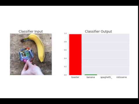](https://youtu.be/i1sp4X57TL4)\n\nLet's take a closer look at how we can actually train such patches. The general idea is very similar to FSGM in the sense that we calculate gradients for the input, and update our adversarial input correspondingly. However, there are also some differences in the setup. Firstly, we do not calculate a gradient for every pixel. Instead, we replace parts of the input image with our patch and then calculate the gradients just for our patch. Secondly, we don't just do it for one image, but we want the patch to work with any possible image. Hence, we have a whole training loop where we train the patch using SGD. Lastly, image patches are usually designed to make the model predict a specific class, not just any other arbitrary class except the true label. For instance, we can try to create a patch for the class \"toaster\" and train the patch so that our pretrained model predicts the class \"toaster\" for any image with the patch in it.\n\nAdditionally, to the setup described above, there are a couple of design choices we can take. For instance, [Brown et al.](https://arxiv.org/pdf/1712.09665.pdf) randomly rotated and scaled the patch during training before placing it at a random position in an input image. This makes the patch more robust to small changes and is necessary if we want to fool a neural network in a real-world application. For simplicity, we will only focus on making the patch robust to the location in the image. Given a batch of input images and a patch, we can add the patch as follows:","metadata":{"id":"qCMQRf6WenfO"}},{"cell_type":"markdown","source":"# 5 Points","metadata":{"id":"QZZVEi6X6Qgt"}},{"cell_type":"code","source":"def place_patch(img, patch):\n \n C, H, W = img.shape\n _, h, w = patch.shape\n\n # patch size smaller than pic\n assert h <= H and w <= W\n\n # random position\n top = np.random.randint(0, H - h + 1)\n left = np.random.randint(0, W - w + 1)\n\n # copy original image\n img_patched = img.clone()\n\n # cverlay patch on image at the selected location\n img_patched[:, top:top + h, left:left + w] = patch\n\n return img_patched\n","metadata":{"id":"heGPwL6TenfO","trusted":true,"execution":{"iopub.status.busy":"2025-05-09T18:12:56.633303Z","iopub.execute_input":"2025-05-09T18:12:56.634209Z","iopub.status.idle":"2025-05-09T18:12:56.639486Z","shell.execute_reply.started":"2025-05-09T18:12:56.634176Z","shell.execute_reply":"2025-05-09T18:12:56.638793Z"}},"outputs":[],"execution_count":null},{"cell_type":"markdown","source":"The patch itself will be an `nn.Parameter` whose values are in the range between $-\\infty$ and $\\infty$. Images are, however, naturally limited in their range, and thus we write a small function that maps the parameter into the image value range of ImageNet:","metadata":{"id":"bod7gkQkenfO"}},{"cell_type":"markdown","source":"# 5 Points","metadata":{"id":"6EF9wLZE6TlZ"}},{"cell_type":"code","source":"TENSOR_MEANS, TENSOR_STD = torch.FloatTensor(mean)[:,None,None], torch.FloatTensor(std)[:,None,None]\ndef patch_forward(patch):\n \n # sigmoid to squash into [0,1]\n patch_img = torch.sigmoid(patch)\n\n # normalize using imageNet statistics\n patch_img = (patch_img - TENSOR_MEANS.to(patch.device)) / TENSOR_STD.to(patch.device)\n\n return patch_img","metadata":{"id":"pvVRh-KXenfO","trusted":true,"execution":{"iopub.status.busy":"2025-05-09T18:12:56.640269Z","iopub.execute_input":"2025-05-09T18:12:56.640537Z","iopub.status.idle":"2025-05-09T18:12:56.666896Z","shell.execute_reply.started":"2025-05-09T18:12:56.640516Z","shell.execute_reply":"2025-05-09T18:12:56.666174Z"}},"outputs":[],"execution_count":null},{"cell_type":"markdown","source":"Before looking at the actual training code, we can write a small evaluation function. We evaluate the success of a patch by how many times we were able to fool the network into predicting our target class. A simple function for this is implemented below.","metadata":{"id":"x0vll2GwenfP"}},{"cell_type":"markdown","source":"# 10 Points","metadata":{"id":"qLj4SRqQ6Vmg"}},{"cell_type":"markdown","source":"Finally, we can look at the training loop. Given a model to fool, a target class to design the patch for, and a size $k$ of the patch in the number of pixels, we first start by creating a parameter of size $3\\times k\\times k$. These are the only parameters we will train, and the network itself remains untouched. We use a simple SGD optimizer with momentum to minimize the classification loss of the model given the patch in the image. While we first start with a very high loss due to the good initial performance of the network, the loss quickly decreases once we start changing the patch. In the end, the patch will represent patterns that are characteristic of the class. For instance, if we would want the model to predict a \"goldfish\" in every image, we would expect the pattern to look somewhat like a goldfish. Over the iterations, the model finetunes the pattern and, hopefully, achieves a high fooling accuracy.","metadata":{"id":"Nyne_WLAenfP"}},{"cell_type":"code","source":"def eval_patch(model, patch, val_loader, target_class):\n \"\"\"\n Evaluate how often the model is fooled into predicting the target class due to the patch.\n \"\"\"\n model = model.to(device)\n model.eval()\n total, fooled_top1, fooled_top5 = 0, 0, 0\n\n with torch.no_grad():\n for imgs, labels in val_loader:\n imgs, labels = imgs.to(device), labels.to(device)\n\n # skip images that are already of the target class\n mask = labels != target_class\n if mask.sum() == 0:\n continue\n imgs, labels = imgs[mask], labels[mask]\n\n batch_size = imgs.size(0)\n preds_1 = torch.zeros(batch_size, device=device)\n preds_5 = torch.zeros(batch_size, device=device)\n\n for _ in range(4):\n patch_img = patch_forward(patch).detach().to(device)\n patched_imgs = torch.stack([\n place_patch(img, patch_img) for img in imgs\n ]).to(device)\n\n outputs = model(patched_imgs)\n top1_preds = outputs.argmax(dim=1)\n top5_preds = torch.topk(outputs, 5, dim=1).indices\n\n preds_1 += (top1_preds == target_class).float()\n preds_5 += (top5_preds == target_class).any(dim=1).float()\n\n fooled_top1 += (preds_1 >= 1).sum().item()\n fooled_top5 += (preds_5 >= 1).sum().item()\n total += batch_size\n\n acc = fooled_top1 / total\n top5 = fooled_top5 / total\n return acc, top5\n","metadata":{"id":"tCU_5dXCenfP","trusted":true,"execution":{"iopub.status.busy":"2025-05-09T18:12:56.667693Z","iopub.execute_input":"2025-05-09T18:12:56.667909Z","iopub.status.idle":"2025-05-09T18:12:56.68484Z","shell.execute_reply.started":"2025-05-09T18:12:56.667888Z","shell.execute_reply":"2025-05-09T18:12:56.684146Z"}},"outputs":[],"execution_count":null},{"cell_type":"markdown","source":"# 15 Points","metadata":{"id":"5c7rdCvY6X4i"}},{"cell_type":"code","source":"def patch_attack(model, target_class, patch_size=64, num_epochs=5):\n \n model.eval()\n\n # use 90% of data for training patch, 10% for evaluation\n train_len = int(len(sub_dataloader.dataset) * 0.9)\n val_len = len(sub_dataloader.dataset) - train_len\n train_set, val_set = torch.utils.data.random_split(sub_dataloader.dataset, [train_len, val_len])\n train_loader = torch.utils.data.DataLoader(train_set, batch_size=32, shuffle=True, num_workers=2)\n val_loader = torch.utils.data.DataLoader(val_set, batch_size=32, shuffle=False, num_workers=2)\n\n # initialize patch parameter\n patch = nn.Parameter(torch.randn(3, patch_size, patch_size))\n\n # optimizer (AdamW)\n optimizer = torch.optim.AdamW([patch], lr=0.005, weight_decay=0.001,)\n\n loss_fn = nn.CrossEntropyLoss()\n\n for epoch in range(num_epochs):\n pbar = tqdm(train_loader, desc=f\"Epoch {epoch+1}/{num_epochs}\")\n for imgs, labels in pbar:\n imgs, labels = imgs.to(device), labels.to(device)\n\n # skip target class images (not fooling them)\n mask = labels != target_class\n if mask.sum() == 0:\n continue\n imgs = imgs[mask]\n\n # forward: place patch\n patch_img = patch_forward(patch)\n patched_imgs = torch.stack([place_patch(img, patch_img) for img in imgs])\n\n # predict and calculate loss\n outputs = model(patched_imgs)\n target_labels = torch.full((patched_imgs.size(0),), target_class, dtype=torch.long, device=device)\n loss = loss_fn(outputs, target_labels)\n\n # backward\n optimizer.zero_grad()\n loss.backward()\n optimizer.step()\n\n pbar.set_postfix(loss=loss.item())\n\n # final validation\n acc, top5 = eval_patch(model, patch, val_loader, target_class)\n return patch.data, {\"acc\": acc, \"top5\": top5}\n","metadata":{"id":"KXKvrik_enfP","trusted":true,"execution":{"iopub.status.busy":"2025-05-09T18:12:56.685693Z","iopub.execute_input":"2025-05-09T18:12:56.685981Z","iopub.status.idle":"2025-05-09T18:12:56.706633Z","shell.execute_reply.started":"2025-05-09T18:12:56.685958Z","shell.execute_reply":"2025-05-09T18:12:56.706091Z"}},"outputs":[],"execution_count":null},{"cell_type":"markdown","source":"To get some experience with what to expect from an adversarial patch attack, we want to train multiple patches for different classes. As the training of a patch can take one or two minutes on a GPU, we have provided a couple of pre-trained patches including their results on the full dataset. The results are saved in a JSON file, which is loaded below.","metadata":{"id":"2BBZtygpenfP"}},{"cell_type":"code","source":"# load evaluation results of the pretrained patches\njson_results_file = os.path.join(CHECKPOINT_PATH, \"patch_results.json\")\njson_results = {}\nif os.path.isfile(json_results_file):\n with open(json_results_file, \"r\") as f:\n json_results = json.load(f)\n\n# if you train new patches, you can save the results via calling this function\ndef save_results(patch_dict):\n result_dict = {cname: {psize: [t.item() if isinstance(t, torch.Tensor) else t\n for t in patch_dict[cname][psize][\"results\"]]\n for psize in patch_dict[cname]}\n for cname in patch_dict}\n with open(os.path.join(CHECKPOINT_PATH, \"patch_results.json\"), \"w\") as f:\n json.dump(result_dict, f, indent=4)","metadata":{"id":"M3TEprXaenfP","trusted":true,"execution":{"iopub.status.busy":"2025-05-09T18:12:56.707309Z","iopub.execute_input":"2025-05-09T18:12:56.707508Z","iopub.status.idle":"2025-05-09T18:12:56.728865Z","shell.execute_reply.started":"2025-05-09T18:12:56.707493Z","shell.execute_reply":"2025-05-09T18:12:56.728246Z"}},"outputs":[],"execution_count":null},{"cell_type":"markdown","source":"Additionally, we implement a function to train and evaluate patches for a list of classes and patch sizes. The pretrained patches include the classes *toaster*, *goldfish*, *school bus*, *lipstick*, and *pineapple*. We chose the classes arbitrarily to cover multiple domains (animals, vehicles, fruits, devices, etc.). We trained each class for three different patch sizes: $32\\times32$ pixels, $48\\times48$ pixels, and $64\\times64$ pixels. We can load them in the two cells below.","metadata":{"id":"U5qtQG1CenfP"}},{"cell_type":"code","source":"def search_in_dict(value, label_images):\n # iterate over dictionary to find the key for a given value\n for key, values in label_images.items():\n if value in values:\n return key\n return None # If value not found, return None\n\n\ndef get_patches(class_names, patch_sizes):\n result_dict = dict()\n\n for cname in class_names:\n result_dict[cname] = {}\n target_class = search_in_dict(cname, label_images) # convert name to ImageNet class index\n\n for psize in patch_sizes:\n print(f\"Processing class '{cname}' with patch size {psize}...\")\n\n patch_file = os.path.join(CHECKPOINT_PATH, f\"patch_{cname}_{psize}.pt\")\n patch_results = json_results.get(cname, {}).get(str(psize), None)\n\n if os.path.isfile(patch_file):\n patch_tensor = torch.load(patch_file, map_location=device)\n else:\n patch_tensor, stats = patch_attack(model, target_class, patch_size=psize)\n torch.save(patch_tensor, patch_file)\n print(f\"Trained and saved patch for class '{cname}', size {psize}\")\n patch_results = [stats[\"acc\"], stats[\"top5\"]]\n\n # If patch file existed but results not yet available, evaluate\n if patch_results is None:\n acc, top5 = eval_patch(model, patch_tensor, sub_dataloader, target_class)\n patch_results = [acc, top5]\n print(f\"Manually evaluated patch for class '{cname}', size {psize}\")\n\n # Store in result dict\n result_dict[cname][str(psize)] = {\n \"patch\": patch_tensor,\n \"results\": patch_results\n }\n\n return result_dict\n","metadata":{"id":"3ZVPZypIenfP","trusted":true,"execution":{"iopub.status.busy":"2025-05-09T18:12:56.729531Z","iopub.execute_input":"2025-05-09T18:12:56.729756Z","iopub.status.idle":"2025-05-09T18:12:56.754016Z","shell.execute_reply.started":"2025-05-09T18:12:56.729737Z","shell.execute_reply":"2025-05-09T18:12:56.753467Z"}},"outputs":[],"execution_count":null},{"cell_type":"markdown","source":"Feel free to add any additional classes and/or patch sizes.","metadata":{"id":"fuY708hbenfP"}},{"cell_type":"markdown","source":"Before looking at the quantitative results, we can actually visualize the patches.","metadata":{"id":"_F0idKgvenfT"}},{"cell_type":"code","source":"class_names = ['toaster', 'goldfish', 'school bus', 'lipstick', 'pineapple']\npatch_sizes = [32, 48, 64]\npatch_dict = get_patches(class_names, patch_sizes)\nsave_results(patch_dict) # Uncomment if you add new class names and want to save the new results","metadata":{"id":"hlsBlFC9enfP","trusted":true,"execution":{"iopub.status.busy":"2025-05-09T18:12:56.754756Z","iopub.execute_input":"2025-05-09T18:12:56.755025Z","iopub.status.idle":"2025-05-09T18:46:53.70221Z","shell.execute_reply.started":"2025-05-09T18:12:56.755004Z","shell.execute_reply":"2025-05-09T18:46:53.701379Z"}},"outputs":[],"execution_count":null},{"cell_type":"markdown","source":"# 5 Points","metadata":{"id":"qDfiC5h76cFx"}},{"cell_type":"code","source":"import matplotlib.pyplot as plt\n\ndef show_patches(patch_dict):\n \"\"\"\n Visualizes trained adversarial patches from the patch dictionary.\n\n Args:\n patch_dict: Dictionary containing patches, keyed by class name and patch size.\n \"\"\"\n num_classes = len(patch_dict)\n num_sizes = len(next(iter(patch_dict.values())))\n \n fig, axes = plt.subplots(num_classes, num_sizes, figsize=(3 * num_sizes, 3 * num_classes))\n\n for row_idx, (class_name, size_dict) in enumerate(patch_dict.items()):\n for col_idx, (patch_size, patch_info) in enumerate(size_dict.items()):\n patch = patch_forward(patch_info[\"patch\"]).detach().cpu()\n patch_img = patch.permute(1, 2, 0).numpy()\n patch_img = (patch_img - patch_img.min()) / (patch_img.max() - patch_img.min()) # Normalize for display\n\n ax = axes[row_idx, col_idx] if num_classes > 1 else axes[col_idx]\n ax.imshow(patch_img)\n ax.axis('off')\n acc, top5 = patch_info[\"results\"]\n ax.set_title(f\"{class_name}\\n{patch_size}px\\nTop1: {acc:.2%}, Top5: {top5:.2%}\")\n\n plt.tight_layout()\n plt.show()\n\nshow_patches(patch_dict)","metadata":{"id":"1k4GjUkjenfT","outputId":"d3516f0b-1422-438e-a131-8e51f668390f","trusted":true,"execution":{"iopub.status.busy":"2025-05-09T18:46:53.703311Z","iopub.execute_input":"2025-05-09T18:46:53.703558Z","iopub.status.idle":"2025-05-09T18:46:57.070739Z","shell.execute_reply.started":"2025-05-09T18:46:53.703535Z","shell.execute_reply":"2025-05-09T18:46:57.0699Z"}},"outputs":[],"execution_count":null},{"cell_type":"markdown","source":"We can see a clear difference between patches of different classes and sizes. In the smallest size, $32\\times 32$ pixels, some of the patches clearly resemble their class. For instance, the goldfish patch clearly shows a goldfish. The eye and the color are very characteristic of the class. Overall, the patches with $32$ pixels have very strong colors that are typical for their class (yellow school bus, pink lipstick, greenish pineapple). The larger the patch becomes, the more stretched the pattern becomes. For the goldfish, we can still spot regions that might represent eyes and the characteristic orange color, but it is not clearly a single fish anymore. For the pineapple, we might interpret the top part of the image as the leaves of pineapple fruit, but it is more abstract than our small patches. Nevertheless, we can easily spot the alignment of the patch to class, even on the largest scale.\n\nLet's now look at the quantitative results.","metadata":{"id":"m3kpUlwqenfT"}},{"cell_type":"code","source":"%%html\n\n","metadata":{"id":"f4ccSfMNenfT","outputId":"915b8a75-a9b4-4853-f107-9840c43a2e62","trusted":true,"execution":{"iopub.status.busy":"2025-05-09T18:46:57.071691Z","iopub.execute_input":"2025-05-09T18:46:57.07235Z","iopub.status.idle":"2025-05-09T18:46:57.07764Z","shell.execute_reply.started":"2025-05-09T18:46:57.072326Z","shell.execute_reply":"2025-05-09T18:46:57.076994Z"}},"outputs":[],"execution_count":null},{"cell_type":"code","source":"import tabulate\nfrom IPython.display import display, HTML\n\ndef show_table(top_1=True):\n i = 0 if top_1 else 1\n table = [[name] + [f\"{(100.0 * patch_dict[name][str(psize)]['results'][i]):4.2f}%\" for psize in patch_sizes]\n for name in class_names]\n display(HTML(tabulate.tabulate(table, tablefmt='html', headers=[\"Class name\"] + [f\"Patch size {psize}x{psize}\" for psize in patch_sizes])))","metadata":{"id":"RvvWRilQenfT","trusted":true,"execution":{"iopub.status.busy":"2025-05-09T18:46:57.07848Z","iopub.execute_input":"2025-05-09T18:46:57.078665Z","iopub.status.idle":"2025-05-09T18:46:57.130959Z","shell.execute_reply.started":"2025-05-09T18:46:57.078651Z","shell.execute_reply":"2025-05-09T18:46:57.130288Z"}},"outputs":[],"execution_count":null},{"cell_type":"markdown","source":"First, we will create a table of top-1 accuracy, meaning that how many images have been classified with the target class as highest prediction?","metadata":{"id":"l9ajy6g2enfT"}},{"cell_type":"code","source":"show_table(top_1=True)","metadata":{"id":"mObFpQetenfT","outputId":"40164751-2053-45bf-aa4e-eb789535da82","trusted":true,"execution":{"iopub.status.busy":"2025-05-09T18:46:57.131674Z","iopub.execute_input":"2025-05-09T18:46:57.131873Z","iopub.status.idle":"2025-05-09T18:46:57.139093Z","shell.execute_reply.started":"2025-05-09T18:46:57.131859Z","shell.execute_reply":"2025-05-09T18:46:57.138474Z"}},"outputs":[],"execution_count":null},{"cell_type":"markdown","source":"The clear trend, that we would also have expected, is that the larger the patch, the easier it is to fool the model. For the largest patch size of $64\\times 64$, we are able to fool the model on almost all images, despite the patch covering only 8% of the image. The smallest patch actually covers 2% of the image, which is almost neglectable. Still, the fooling accuracy is quite remarkable. A large variation can be however seen across classes. While *school bus* and *pineapple* seem to be classes that were easily predicted, *toaster* and *lipstick* seem to be much harder for creating a patch. It is hard to intuitively explain why our patches underperform on those classes. Nonetheless, a fooling accuracy of >40% is still very good for such a tiny patch.\n\nLet's also take a look at the top-5 accuracy:","metadata":{"id":"PQ6cOHPmenfT"}},{"cell_type":"code","source":"show_table(top_1=False)","metadata":{"id":"akt_xV3DenfU","outputId":"51647046-3a99-4949-e652-eb4ee2c97278","trusted":true,"execution":{"iopub.status.busy":"2025-05-09T18:46:57.139873Z","iopub.execute_input":"2025-05-09T18:46:57.140228Z","iopub.status.idle":"2025-05-09T18:46:57.155762Z","shell.execute_reply.started":"2025-05-09T18:46:57.14021Z","shell.execute_reply":"2025-05-09T18:46:57.155254Z"}},"outputs":[],"execution_count":null},{"cell_type":"markdown","source":"We see a very similar pattern across classes and patch sizes. The patch size $64$ obtains >99.7% top-5 accuracy for any class, showing that we can almost fool the network on any image. A top-5 accuracy of >70% for the hard classes and small patches is still impressive and shows how vulnerable deep CNNs are to such attacks.\n\nFinally, let's create some example visualizations of the patch attack in action.","metadata":{"id":"sk61i2NZenfU"}},{"cell_type":"markdown","source":"# 10 Points","metadata":{"id":"9azhdwSs6fwr"}},{"cell_type":"code","source":"import matplotlib.pyplot as plt\nimport torchvision.transforms.functional as TF\n\ndef perform_patch_attack(patch, model, val_loader, target_class, device='cuda', num_images=3):\n model = model.to(device).eval()\n patch = patch.to(device)\n patch_img = patch_forward(patch).detach()\n\n images_shown = 0\n\n with torch.no_grad():\n for imgs, labels in val_loader:\n imgs, labels = imgs.to(device), labels.to(device)\n\n for idx in range(imgs.size(0)):\n if labels[idx].item() == target_class:\n continue # skip true target class\n\n img = imgs[idx]\n label = labels[idx].item()\n\n # Apply patch\n patched = place_patch(img, patch_img)\n\n # Get predictions\n orig_out = model(img.unsqueeze(0))\n patch_out = model(patched.unsqueeze(0))\n\n orig_pred = orig_out.argmax(dim=1).item()\n patch_pred = patch_out.argmax(dim=1).item()\n\n # Convert for plotting\n unnorm = transforms.Normalize(mean=[-m/s for m, s in zip(mean, std)],\n std=[1/s for s in std])\n img_disp = TF.to_pil_image(unnorm(img.cpu()))\n patch_disp = TF.to_pil_image(unnorm(patched.cpu()))\n\n # Plotting\n fig, axs = plt.subplots(1, 2, figsize=(8, 4))\n axs[0].imshow(img_disp)\n axs[0].set_title(f\"Original: {label_images.get(orig_pred)[0]}\")\n axs[0].axis('off')\n\n axs[1].imshow(patch_disp)\n axs[1].set_title(f\"Patched: {label_images.get(patch_pred)[0]}\")\n axs[1].axis('off')\n\n plt.tight_layout()\n plt.show()\n\n images_shown += 1\n if images_shown >= num_images:\n return\n","metadata":{"id":"yNxj8CufenfU","trusted":true,"execution":{"iopub.status.busy":"2025-05-09T19:00:29.834703Z","iopub.execute_input":"2025-05-09T19:00:29.834972Z","iopub.status.idle":"2025-05-09T19:00:29.844576Z","shell.execute_reply.started":"2025-05-09T19:00:29.834952Z","shell.execute_reply":"2025-05-09T19:00:29.843988Z"}},"outputs":[],"execution_count":null},{"cell_type":"code","source":"perform_patch_attack(\n patch=patch_dict['goldfish'][str(32)]['patch'],\n model=model,\n val_loader=sub_dataloader,\n target_class=search_in_dict('goldfish', label_images)\n)\n","metadata":{"id":"pO3nFz-uenfU","outputId":"e6d4df9c-d616-410d-b141-723317d72bcb","trusted":true,"execution":{"iopub.status.busy":"2025-05-09T19:02:01.714198Z","iopub.execute_input":"2025-05-09T19:02:01.714921Z","iopub.status.idle":"2025-05-09T19:02:06.956229Z","shell.execute_reply.started":"2025-05-09T19:02:01.714896Z","shell.execute_reply":"2025-05-09T19:02:06.955294Z"}},"outputs":[],"execution_count":null},{"cell_type":"markdown","source":"The tiny goldfish patch can change all of the predictions to \"goldfish\" as top class. Note that the patch attacks work especially well if the input image is semantically similar to the target class (e.g. a fish and the target class \"goldfish\" works better than an airplane image with that patch). Nevertheless, we can also let the network predict semantically dis-similar classes by using a larger patch:","metadata":{"id":"VFEoVsUZenfU"}},{"cell_type":"code","source":"perform_patch_attack(\n patch=patch_dict['school bus'][str(64)]['patch'],\n model=model,\n val_loader=sub_dataloader,\n target_class=search_in_dict('school bus', label_images)\n)","metadata":{"id":"WgNe3aWbenfU","outputId":"5ef3db60-bd51-4507-fa01-96adf250c517","trusted":true,"execution":{"iopub.status.busy":"2025-05-09T19:02:06.957887Z","iopub.execute_input":"2025-05-09T19:02:06.958189Z","iopub.status.idle":"2025-05-09T19:02:12.279315Z","shell.execute_reply.started":"2025-05-09T19:02:06.958168Z","shell.execute_reply":"2025-05-09T19:02:12.278521Z"}},"outputs":[],"execution_count":null},{"cell_type":"markdown","source":"Although none of the images have anything to do with an American school bus, the high confidence of often 100% shows how powerful such attacks can be. With a few lines of code and access to the model, we were able to generate patches that we add to any image to make the model predict any class we want.","metadata":{"id":"qnoEM5AxenfU"}},{"cell_type":"markdown","source":"### Transferability of white-box attacks\n\nFGSM and the adversarial patch attack were both focused on one specific image. However, can we transfer those attacks to other models? The adversarial patch attack as proposed in [Brown et al.](https://arxiv.org/pdf/1712.09665.pdf), was originally trained on multiple models, and hence was also able to work on many different network architecture. But how different are the patches for different models anyway? For instance, let's evaluate some of our patches trained above on a different network, e.g. DenseNet121.","metadata":{"id":"zrRzlIhQenfU"}},{"cell_type":"markdown","source":"# 15 Points","metadata":{"id":"LqvUERjL6jIa"}},{"cell_type":"code","source":"from torchvision import models\n\n# load DenseNet121 pretrained on ImageNet\ntransfer_model = models.densenet121(pretrained=True)\n\n# don’t compute or store gradients\nfor param in transfer_model.parameters():\n param.requires_grad = False\n\ntransfer_model = transfer_model.to(device)\ntransfer_model.eval()\n\nprint(transfer_model)","metadata":{"id":"VW6lbGexenfU","trusted":true,"execution":{"iopub.status.busy":"2025-05-09T19:02:53.848977Z","iopub.execute_input":"2025-05-09T19:02:53.849845Z","iopub.status.idle":"2025-05-09T19:02:54.372838Z","shell.execute_reply.started":"2025-05-09T19:02:53.849817Z","shell.execute_reply":"2025-05-09T19:02:54.371914Z"}},"outputs":[],"execution_count":null},{"cell_type":"markdown","source":"Feel free to change the class name and/or patch size below to test out different patches.","metadata":{"id":"8e5XWXB1enfV"}},{"cell_type":"code","source":"class_name = 'pineapple'\npatch_size = 64\nprint(f\"Testing patch \\\"{class_name}\\\" of size {patch_size}x{patch_size}\")\n\nresults = eval_patch(transfer_model,\n patch_dict[class_name][str(patch_size)][\"patch\"],\n val_loader=sub_dataloader,\n target_class=search_in_dict(class_name, label_images))\n\nprint(f\"Top-1 fool accuracy: {(results[0] * 100.0):4.2f}%\")\nprint(f\"Top-5 fool accuracy: {(results[1] * 100.0):4.2f}%\")","metadata":{"id":"bHbVoMTuenfV","outputId":"0bca9c24-b79c-4db7-dc5d-95c5a09e007f","trusted":true,"execution":{"iopub.status.busy":"2025-05-09T19:03:33.624333Z","iopub.execute_input":"2025-05-09T19:03:33.625182Z","iopub.status.idle":"2025-05-09T19:04:58.546524Z","shell.execute_reply.started":"2025-05-09T19:03:33.625156Z","shell.execute_reply":"2025-05-09T19:04:58.545743Z"}},"outputs":[],"execution_count":null},{"cell_type":"markdown","source":"Although the fool accuracy is significantly lower than on the original ResNet34, it still has a considerable impact on DenseNet although the networks have completely different architectures and weights. If you would compare more patches and models, some would work better than others. However, one aspect which allows patch attacks to generalize well is if all the networks have been trained on the same data. In this case, all networks have been trained on ImageNet. Dataset biases make the networks recognize specific patterns in the underlying image data that humans would not have seen, and/or only work for the given dataset. This is why the knowledge of what data has been used to train a specific model is already worth a lot in the context of adversarial attacks.","metadata":{"id":"U4EyOfx4enfV"}},{"cell_type":"markdown","source":"## Protecting against adversarial attacks\n\nThere are many more attack strategies than just FGSM and adversarial patches that we haven't discussed and implemented ourselves here. However, what about the other perspective? What can we do to *protect* a network against adversarial attacks? The sad truth to this is: not much.\n\nWhite-box attacks require access to the model and its gradient calculation. The easiest way of preventing this is by ensuring safe, private storage of the model and its weights. However, some attacks, called black-box attacks, also work without access to the model's parameters, or white-box attacks can also generalize as we have seen above on our short test on transferability.\n\nSo, how could we eventually protect a model? An intuitive approach would to train/finetune a model on such adversarial images, leading to an adversarial training similar to a GAN. During training, we would pretend to be the attacker, and use for example FGSM as an augmentation strategy. However, this usually just ends up in an oscillation of the defending network between weak spots. Another common trick to increase robustness against adversarial attacks is defensive distillation ([Papernot et al.](https://arxiv.org/pdf/1511.04508.pdf)). Instead of training the model on the dataset labels, we train a secondary model on the softmax predictions of the first one. This way, the loss surface is \"smoothed\" in the directions an attacker might try to exploit, and it becomes more difficult for the attacker to find adversarial examples. Nevertheless, there hasn't been found the one, true strategy that works against all possible adversarial attacks.\n\nWhy are CNNs, or neural networks in general, so vulnerable to adversarial attacks? While there are many possible explanations, the most intuitive is that neural networks don't know what they don't know. Even a large dataset represents just a few sparse points in the extremely large space of possible images. A lot of the input space has not been seen by the network during training, and hence, we cannot guarantee that the prediction for those images is any useful. The network instead learns a very good classification on a smaller region, often referred to as manifold, while ignoring the points outside of it. NNs with uncertainty prediction could potentially help to discover what the network does not know.\nAnother possible explanation lies in the activation function. As we know, most CNNs use ReLU-based activation functions. While those have enabled great success in training deep neural networks due to their stable gradient for positive values, they also constitute a possible flaw. The output range of a ReLU neuron can be arbitrarily high. Thus, if we design a patch or the noise in the image to cause a very high value for a single neuron, it can overpower many other features in the network. Thus, although ReLU stabilizes training, it also offers a potential point of attack for adversaries.","metadata":{"id":"pyybhYl4enfV"}}]} 
