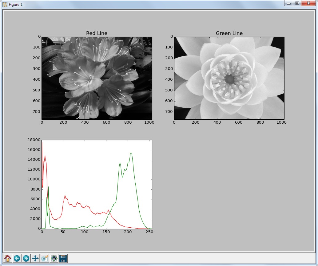
{"metadata":{"kernelspec":{"language":"python","display_name":"Python 3","name":"python3"},"language_info":{"pygments_lexer":"ipython3","nbconvert_exporter":"python","version":"3.6.4","file_extension":".py","codemirror_mode":{"name":"ipython","version":3},"name":"python","mimetype":"text/x-python"}},"nbformat_minor":4,"nbformat":4,"cells":[{"cell_type":"code","source":"import numpy as np # linear algebra\nimport pandas as pd # data processing, CSV file I/O (e.g. pd.read_csv)\nimport os\nimport matplotlib.pyplot as plt\nimport seaborn as sns\nfrom PIL import Image\nfrom glob import glob\nfrom tqdm import tqdm\nimport cv2","metadata":{"_uuid":"8f2839f25d086af736a60e9eeb907d3b93b6e0e5","_cell_guid":"b1076dfc-b9ad-4769-8c92-a6c4dae69d19","scrolled":true,"trusted":true},"execution_count":null,"outputs":[]},{"cell_type":"markdown","source":"# Reference : [Original Notebook](https://www.kaggle.com/frlemarchand/generate-masks-from-weak-image-level-labels)\n\nhttps://www.kaggle.com/frlemarchand/generate-masks-from-weak-image-level-labels \nI refer to this notebook. \nI study many function, code and knowledge based on this notebook.\nAnd then I add more information and knowledge by myself. \n\nThanks for \n[@Francois Lemarchand](https://www.kaggle.com/frlemarchand)\n\n### 이 노트북은 학습을 위해 위의 참조 노트북을 참고하고, 번역하였으며, 추가로 공부한 내용과 지식을 정리한 노트북입니다.","metadata":{}},{"cell_type":"markdown","source":"## Introduction\n\n이 노트북은 데이터를 불러오는 몇몇 함수들을 소개하는 것과, 학습 이미지에 존재하는 모든 세포의 클래스별 마스크를 생성하는 것을 목표로 합니다. \n각 클래스별 마스크(instance segmentation masks) 를 생성함으로써, 우리는 세포를 개별적으로 분석할 수 있고, 전체 이미지를 대상으로 주어진 한개 또는 여러개의 레이블과 연관지어볼 수 있습니다. ","metadata":{}},{"cell_type":"code","source":"data_dir = '../input/hpa-single-cell-image-classification/'\ntrain_dir = data_dir + 'train/'\ntrain_df = pd.read_csv(\"../input/hpa-single-cell-image-classification/train.csv\")\ntrain_df","metadata":{"scrolled":true,"trusted":true},"execution_count":null,"outputs":[]},{"cell_type":"markdown","source":"# Load the images and apply a binary mask","metadata":{}},{"cell_type":"code","source":"def get_binary_mask(img):\n \"\"\" key : RGB 이미지를 Gray scale 이미지로 변환하는 함수\n \n < get_binary_mask 함수 >\n 이진 segmentation (각 픽셀을 이진으로 분류하는 것 = 흑백으로 분류)을 하기 위해 \n Otsu threshold를 적용하기 전,\n RGB 이미지를 gray scale 이미지로 바꾸는 함수\n \n - 각 픽셀을 이진으로 분류하기 위해서는 gray scale 이미지가 필요\n - Otsu threshold : 픽셀을 이진 분류하는 otsu threshold.\n \"\"\"\n blurred_img = cv2.GaussianBlur(img, (25,25), 0)\n gray_img = cv2.cvtColor(blurred_img, cv2.COLOR_RGBA2GRAY)\n ret, otsu = cv2.threshold(gray_img, 0, 255, cv2.THRESH_BINARY + cv2.THRESH_OTSU)\n \n kernel = np.ones((40,40), np.uint8)\n closed_mask = cv2.morphologyEx(otsu, cv2.MORPH_CLOSE, kernel) # img, opening 방식, kernel 사이즈\n \n return closed_mask\n\n# 이미지를 otsu threshold에 기반한 grayscale 이미지로 바꾼후, \n# 노이즈 제거를 한번 해준 mask(binary segmentation image)를 리턴","metadata":{"scrolled":true,"trusted":true},"execution_count":null,"outputs":[]},{"cell_type":"markdown","source":"### [Otsu threshold](https://opencv-python.readthedocs.io/en/latest/doc/09.imageThresholding/imageThresholding.html)\n\n```py\ncv2.threshold(src, thres, maxval, type)\n- src : input_image 로 single_channel 이미지 (그레이 스케일)\n- thresh : 임계값\n- maxval : 임계값을 넘었을 때 적용할 value\n- type : thresholding type : type 에 따라 이진 색깔의 타입을 지정할 수 있다.\n\ncv2.adaptiveThreshold(src, maxValue, adaptiveMethod, thresholdType, blockSize, C)\n- 일부 영역이 완전히 흰색 또는 검정색으로 보여지므로 이것을 해결하기 위한 함수\n```\n\nOtsu 의 이진화 \n: thresholding 처리에서 임계값은 사용자가 결정하여 parameter 로 전달. by trial and error 방식 \n: bimodal image(히스토그램으로 분석하면 2개의 peak 가 있는 이미지)의 경우는 히스토그램에서 임계값을 어느정도 정확히 계산할 수 있다. \n\nOtsu의 이진화(Otsu's Binarization)란 bimodal image 에서 임계값을 자동으로 계산해주는 것.\n\n### [cv2.morphologyEx](https://webnautes.tistory.com/1257)\nOpenCV 에서 제공하는 함수 : Erosion, Dilation, Opening, Closing \n1. Erosion : 바이너리 이미지에서 흰색 '오브젝트'의 외곽 픽셀을 0(검은색)으로 만든다.(사진 전체의 외곽 X) = 가늘게\n2. Dilation : Erosion 과 반대. 흰색 오브젝트의 외곽 픽셀을 1로 만든다. = 두껍게\n3. Opening : Erosion 연산 다음에 Dilation 연산을 적용.(한번 지우고도 존재하는 것들을 두껍게) 이미지 상의 노이즈(작은 흰색)를 제거하는데 사용 \n4. Closing : Dilation 연산 다음에 Erosion 연산을 적용. 흰색 오브젝트에 있는 작은 검은색 구멍들을 메우는데 사용.\n```py\ncv2.erode()\ncv2.dilate()\ncv2.morphologyEx(img, cv2.MORPH_OPEN, kernel)\ncv2.morphologyEx(img, cv2.MORPH_CLOSE, kernel)\n``` \nkernel : filter 크기","metadata":{}},{"cell_type":"code","source":"def load_RGBY_image(image_id_path):\n \"\"\" key : 모든 색상의 이미지를 합한 array 를 리턴. \n Load and stack the channels that are stored separately.\n \"\"\"\n red_image = cv2.imread(image_id_path+\"_red.png\", cv2.IMREAD_UNCHANGED)\n green_image = cv2.imread(image_id_path+\"_green.png\", cv2.IMREAD_UNCHANGED)\n blue_image = cv2.imread(image_id_path+\"_blue.png\", cv2.IMREAD_UNCHANGED)\n yellow_image = cv2.imread(image_id_path+\"_yellow.png\", cv2.IMREAD_UNCHANGED)\n\n stacked_images = np.transpose(np.array([red_image, green_image, blue_image, yellow_image]), \n (1,2,0))\n \n return stacked_images\n\n# cv2.IMREAD_UNCHANGED : alpha channel 포함. source image 로 읽어들임 ARGB\n# TODO : 근데 여기선 왜 1차원이지?\n# np.transpose : W x H x C -> C x W x H 로 변경","metadata":{"scrolled":true,"trusted":true},"execution_count":null,"outputs":[]},{"cell_type":"code","source":"fig, axes = plt.subplots(1,2,figsize=(12,4))\naxes[0].imshow(stacked_images[:,:,:3]) # RGB image\naxes[1].imshow(binary_mask)\nplt.show();","metadata":{"scrolled":true,"trusted":true},"execution_count":null,"outputs":[]},{"cell_type":"code","source":"cv2.imread(image_id_path+'_red.png', cv2.IMREAD_COLOR).shape","metadata":{"scrolled":true,"trusted":true},"execution_count":null,"outputs":[]},{"cell_type":"code","source":"# sample 확인\nimage_id_path = train_dir + train_df.iloc[0]['ID']\nstacked_images = load_RGBY_image(image_id_path) # 4 channel : red, green, blue, yellow\nbinary_mask = get_binary_mask(stacked_images)\n\nprint(f\"stacked_images.shape : {stacked_images.shape}\\nbinary_mask.shape : {binary_mask.shape}\")","metadata":{"scrolled":true,"trusted":true},"execution_count":null,"outputs":[]},{"cell_type":"markdown","source":"binary mask 는 RGB+Y 이미지를 기준으로 binary masking 을 통해 추출.","metadata":{}},{"cell_type":"markdown","source":"## Generate instance masks and convert to RLE encoding\n```py\ndef rle_encoding(x)\ndef get_instance_masks(binary_mask)\n```","metadata":{}},{"cell_type":"code","source":"def rle_encoding(x):\n \n \"\"\" Run-length encoding : https://en.wikipedia.org/wiki/Run-length_encoding\n \n 마스크를 저장하기 쉬운 형식으로 바꾸는 것\n RLE encoding 된 마스크를 모델에 input 시킨다.\n \n ex) WWWBBBBWWCCCCCC = 3W4B2W6C\n \"\"\"\n \n dots = np.where(x.T.flatten() == 255)[0]\n run_lengths = []\n prev = -2\n \n for b in dots:\n if (b > prev + 1):\n run_lengths.extend((b+1, 0))\n run_lengths[-1] += 1\n prev = b # 한칸 이상 동떨어져 있을 경우 length 리셋\n \n return ' '.join([str(x) for x in run_lengths])","metadata":{"scrolled":true,"trusted":true},"execution_count":null,"outputs":[]},{"cell_type":"code","source":"def get_instance_masks(binary_mask):\n \"\"\"\n 바이너리 마스크를 input 받아서,\n 작은 아이템은 걸러내고, 큰 binary larget object 의 독립된 마스크를 생성한다.\n \"\"\"\n contours = cv2.findContours(binary_mask, \n cv2.RETR_TREE,\n cv2.CHAIN_APPROX_SIMPLE)\n instance_masks = []\n for contour in contours[0]:\n if cv2.contourArea(contour) > 100: # 형태의 넓이 구하기\n instance_contour = np.zeros(binary_mask.shape) # 일단 전체 이미지 크기만큼\n cv2.drawContours(instance_contour, [contour], \n 0, 255, thickness = cv2.FILLED)\n \n encoded_cell_mask = rle_encoding(instance_contour)\n instance_masks.append(encoded_cell_mask)\n \n return instance_masks\n \n# parameter 설명은 링크참조\n# cv2.RETR_TREE : 모든 contours line 을 찾으며, 모든 hierachy 관계를 구성함.\n# cv2.CHAIN_APPROX_SIMPLE : contours line 을 그릴 수 있는 point 만 저장(ex: 사각형이면 4개 포인트)","metadata":{"scrolled":true,"trusted":true},"execution_count":null,"outputs":[]},{"cell_type":"markdown","source":"### [Contours](https://opencv-python.readthedocs.io/en/latest/doc/15.imageContours/imageContours.html) \n: cv2.findContours, cv2.contourArea, cv2.drawContours \n\n* **contours** : 동일한 색 또는 동일한 강도를 가지고 있는 영역의 경계선을 연결한 선 : like 등고선\n - 정확도를 높히기 위해서 Binary Image 를 사용. Threshold 나 canny edge 를 선처리로 수행\n - `cv2.findContours()` 함수는 원본 이미지를 직접 수정하기 때문에, 원본 이미지를 보존하려면 Copy 해서 사용\n - OpenCV 에서는 contours 를 찾는 것은 검은색 배경에서 하얀색 대상을 찾는 것. So, 대상 = 흰색, 배경 = 검은색\n\n**Find & Draw Contours**\n```py\ncv2.findContours(image, mode, method[, contours[, hierarchy[, offset]]]) → image, contours, hierarchy\n\ncv2.drawContours(image, contours, contourIdx, color[, thickness[, lineType[, hierarchy[, maxLevel[, offset]]]]]) → dst\n\n# parameter 는 링크 참조\n```\n\n[이미지 Contour 응용 링크](https://m.blog.naver.com/PostView.nhn?blogId=samsjang&logNo=220516822775&proxyReferer=https:%2F%2Fwww.google.com%2F)","metadata":{}},{"cell_type":"markdown","source":"## Add the RLE encoding to the existing training dataframe\n\ntrain_df 에 RLE encoding 값을 추가하자","metadata":{}},{"cell_type":"markdown","source":"### 1) 제대로 된 시작 전에 각 과정을 하나하나 뜯어보자","metadata":{}},{"cell_type":"code","source":"train_df[:20].head(5) # iterrows 로 행을 하나씩 불러올 dataframe","metadata":{"scrolled":true,"trusted":true},"execution_count":null,"outputs":[]},{"cell_type":"code","source":"# 아래 process 예시 및 시각화\nfor idx, item in train_df.iterrows():\n image_id_path = train_dir+item.ID\n break\n \nstacked_images = load_RGBY_image(image_id_path)\nbinary_mask = get_binary_mask(stacked_images)\ninstance_masks = get_instance_masks(binary_mask)\n\nprint(f\"stacked_images.shape : {stacked_images.shape}\\nbinary_mask.shape : {binary_mask.shape}\")","metadata":{"scrolled":true,"trusted":true},"execution_count":null,"outputs":[]},{"cell_type":"code","source":"fig, axes = plt.subplots(1,2,figsize=(12,4))\naxes[0].imshow(stacked_images[:,:,:3]) # RGB image\naxes[1].imshow(binary_mask)\nplt.show();","metadata":{"trusted":true},"execution_count":null,"outputs":[]},{"cell_type":"code","source":"# get_instance_mask 함수 내부\n\n# contours (라인 따내기)\ncontours = cv2.findContours(binary_mask, # image\n cv2.RETR_TREE, # contours 라인, 모든 hierachy 관계 구성 = 모든 경계에 컨투어를 그림\n cv2.CHAIN_APPROX_SIMPLE) \n# contours line 을 그릴 수 있는 포인트 저장, 4각형은 4개. 많을 경우, 말 그대로 많기 때문에.\ncontours[1]","metadata":{"trusted":true},"execution_count":null,"outputs":[]},{"cell_type":"markdown","source":"contours[1] = hierachy\n\n|인덱스|다음(next)|이전(prev)|자식(First Child)|부모(parent)|\n|:-|:-:|:-:|:-:|:-:|\n|0|1|-1|-1|-1|\n|1|2|0|-1|-1|\n|2|3|1|-1|-1|\n|3|4|2|-1|-1|\n|4|-1|3|-1|-1|\n\n|인덱스|행|의미|다음|이전|\n|:-:|:-:|:-:|:-:|:-:|\n|인덱스 0 | 0번째 행 | 첫 번째 도형의 컨투어 | 1 = 다음 도형은 1행| 의미없음 |\n|인덱스 1 | 1번째 행 | 두 번째 도형의 컨투어 | 2 = 다음 도형은 2행| 0 = 이전 도형은 0행|\n|인덱스 2 | 2번째 행 | 세 번째 도형의 컨투어 | 3 = 다음 도형은 3행| 1 = 이전 도형은 1행|\n|인덱스 3 | 3번째 행 | 네 번째 도형의 컨투어 | 4 = 다음 도형은 4행| 2 = 이전 도형은 2행|\n|인덱스 4 | 4번째 행 | 다섯 번째 도형의 컨투어 | -1 = 다음 도형은 없음| 3 = 이전 도형은 3행|\n\n\n\n-1 : 의미없음 \n(이 contours hierachy 에서는 자식과 부모가 모두 -1 이므로 표 설명에서 제외함)\n\n자식과 부모 관련 계층은 참고링크 참조 :\n[참고 링크](https://bkshin.tistory.com/entry/OpenCV-22-%EC%BB%A8%ED%88%AC%EC%96%B4Contour)\n\n \n\n이처럼 그림을 그릴 경우 번개 하나에 다양한 방식으로 컨투어를 감싸는 그림을 그릴 수 있음","metadata":{}},{"cell_type":"code","source":"for i in contours[0]:\n print(i.shape)\n# 5개의 라인을 따냈다. = contours 는 검은색 배경에서 흰색을 찾는 것\n# 한붓그리기로 그릴 수 있는 물체 덩어리를 총 5개 찾았다는 말.","metadata":{"trusted":true},"execution_count":null,"outputs":[]},{"cell_type":"markdown","source":"예정된 코드 예시\n```py\ninstance_masks = []\nfor contour in contours[0]: # 현재 5개\n if cv2.contourArea(contour) > 100: # 찾은 영역이 매우 작다면, 패스하겠다.\n instance_contour = np.zeros(binary_mask.shape) # contour 마다 새로운 도화지\n # 일단 전체 이미지 크기만큼 0 array생성(배경) = 윤곽선 그리기 준비\n cv2.drawContours(instance_contour, # 입력 영상(검은색 도화지)\n [contour], # 그림 그릴 컨투어 배열 = contours\n 0, # 그림 그릴 컨투어 인덱스 = contours[0]\n 255, # 색상 값 = 여기서는 흰색으로 통일\n thickness = cv2.FILLED)\n \n encoded_cell_mask = rle_encoding(instance_contour) # \n instance_masks.append(encoded_cell_mask)\n```","metadata":{}},{"cell_type":"code","source":"# contours 5 개 중 하나씩 테스트 시각화 해보자\ninstance_masks = []\ncontour = contours[0][0] # 1/5\nif cv2.contourArea(contour) > 100:\n instance_contour = np.zeros(binary_mask.shape)\n cv2.drawContours(instance_contour, [contour], 0, 255, thickness = cv2.FILLED)\n \nplt.imshow(instance_contour)\nplt.title('instance_contour visualization 1/5')\nplt.show();","metadata":{"trusted":true},"execution_count":null,"outputs":[]},{"cell_type":"code","source":"print(f\"instance_contou unique value : {np.unique(instance_contour)}\")\nprint(f\"instance_contour.shape : {instance_contour.shape}\")\nall_pixels = instance_contour.shape[0] * instance_contour.shape[1]\nprint(f\"all pixel length : {all_pixels}\")","metadata":{"trusted":true},"execution_count":null,"outputs":[]},{"cell_type":"code","source":"# RLE_encoding 함수 안으로\n\ntotal = len(np.where(instance_contour.T.flatten() == 255)[0])\nprint(f\"흰색인 인덱스의 픽셀 수 : {total}\")\nprint(f\"비율 : {(total / all_pixels):.4f}\")\ndots = np.where(instance_contour.T.flatten() == 255)[0]\nprint(f\"\\n dots(index) : {dots}\")\nprint(f\"\\tdots : instance contour 를 전치하고 flatten 시킨 후, 흰색인 것들의 인덱스 값만 뽑아낸 것\")","metadata":{"trusted":true},"execution_count":null,"outputs":[]},{"cell_type":"code","source":"# x = instance_contour\nrun_lengths = []\nprev = -2\nfor b in dots:\n if (b > prev + 1): # b 가 0 이상이면, \n run_lengths.extend((b+1, 0)) # \n run_lengths[-1] += 1\n prev = b\nrle_sample = ' '.join([str(x) for x in run_lengths])\nlen(rle_sample)","metadata":{"trusted":true},"execution_count":null,"outputs":[]},{"cell_type":"code","source":"rle_sample[:500]\n# encoded_cell_mask = rle_encoding(instance_contour)\n# encoded_cell_mask \n# 이 과정을 거친 것","metadata":{"trusted":true},"execution_count":null,"outputs":[]},{"cell_type":"markdown","source":"### 결론\n\n이러한 과정을 4번 더 반복하여 이미지에 해당하는 하나의 rle_encoding 총집합 을 만든다.","metadata":{}},{"cell_type":"markdown","source":"### 2) 프로세스 진행","metadata":{}},{"cell_type":"code","source":"process_RLE_for = 20\ntrain_df[\"RLE_encoding\"] = \"\"\n\nwith tqdm(total=process_RLE_for) as pbar: \n for idx, item in train_df[:process_RLE_for].iterrows():\n image_id_path = train_dir+item.ID\n\n stacked_images = load_RGBY_image(image_id_path)\n binary_mask = get_binary_mask(stacked_images)\n instance_masks = get_instance_masks(binary_mask)\n\n train_df.at[idx, \"RLE_encoding\"] = str(instance_masks)\n pbar.update(1) # to 20(total)\n \n \n# iterrows : 첫 번째 변수 idx 에 인덱스를 받고, item 은 열의 행에 하나씩 접근하여 출력","metadata":{"scrolled":true,"trusted":true},"execution_count":null,"outputs":[]},{"cell_type":"markdown","source":"Manual control of `tqdm()` updates using a `with` statement: \nwith 구문을 사용해서 tqdm 을 수동으로 컨트롤한다. update() 로 수동으로 진행률을 증가시킨다. \n```py\nwith tqdm(total=100) as pbar:\n for i in range(10):\n sleep(0.1)\n pbar.update(10)\n-------------------------------------\npbar = tqdm(total=100)\nfor i in range(10):\n sleep(0.1)\n pbar.update(10)\npbar.close()\n```\n[link](https://github.com/tqdm/tqdm)","metadata":{}},{"cell_type":"code","source":"train_df.loc[15:25] # 20개만 했으므로","metadata":{"scrolled":true,"trusted":true},"execution_count":null,"outputs":[]},{"cell_type":"markdown","source":"## 이미지 히스토그램\n\n학습 이미지의 모든 세포에 대해 개별 마스크를 생성함으로써, 이미지 분석을 실시할 수 있다. \n아래는, 모든 세포와 RGB 채널의 색 분포를 시각화하였다. \n세포의 클래스를 분별하는 방법은 색 분포 signature 에 기반하여 clustering 하는 방법도 있다.","metadata":{}},{"cell_type":"code","source":"def plot_color_distribution(isolated_cell_img):\n color = ('r', 'g', 'b', 'y')\n for i, col in enumerate(color):\n histr = cv2.calcHist([isolated_cell_img],[i], None, [256], [1, 256])\n plt.plot(histr, color = col)\n plt.xlim([1, 256])\n plt.show();","metadata":{"scrolled":true,"trusted":true},"execution_count":null,"outputs":[]},{"cell_type":"markdown","source":"### [Histogram (OpenCV, Matplotlib)](https://opencv-python.readthedocs.io/en/latest/doc/19.imageHistograms/imageHistograms.html)\nOpenCV 와 Matplotlib 를 이용하여 Histogram 을 찾을 수 있다.\n\n* Histogram : 이미지의 밝기의 분포를 그래프로 표현한 방식. 이미지 전체의 밝기 분포와 채도(색의 밝고 어두움)를 알 수 있다.\n```py\ncv2.calcHist(images, channels, mask, histSize, ranges[, hist[, accumulate]])\n```\n \n(좌측 이미지) \n2가지 이미지를 grayscale 로 읽어 빛의 세기 분포를 보여주는 예제(출처 : opencv-python.readthedocs.io) \nRed Line이미지는 전체적으로 어둡기 때문에 히스토그램에서 좌측의 분포가 높고, Green Line 이미지는 전체적으로 밝기 때문에 오른쪽의 분포가 높습니다. \n\n(우측 이미지) \n이미지의 특정영역의 히스토그램을 분석하기 위해서 mask 를 적용할 수 있다. \nred : 원본이미지 히스토그램, blue : mask 적용된 히스토그램\n\n
 \n
\n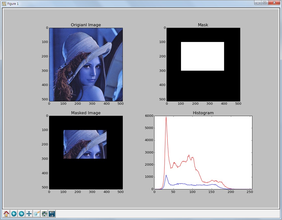 \n\n\n","metadata":{}},{"cell_type":"code","source":"def analyze_individual_cells(binary_mask, original_image): \n \n contours = cv2.findContours(binary_mask,\n cv2.RETR_TREE,\n cv2.CHAIN_APPROX_SIMPLE)\n \n for contour in contours[0]:\n if cv2.contourArea(contour) > 100:\n x, y, width, height = cv2.boundingRect(contour)\n \n instance_contour = np.zeros(binary_mask.shape)\n cv2.drawContours(instance_contour, [contour], 0, 255, thickness = cv2.FILLED)\n \n isolated_cell_image = np.zeros(binary_mask.shape)\n isolated_cell_image = cv2.bitwise_and(original_image, original_image, mask = instance_contour.astype('uint8'))\n \n plt.imshow(isolated_cell_image[y : y+height, x : x+width, :3])\n plt.show()\n plot_color_distribution(isolated_cell_image[y:y+height, x:x+width])","metadata":{"scrolled":true,"trusted":true},"execution_count":null,"outputs":[]},{"cell_type":"markdown","source":"### [비트연산](https://opencv-python.readthedocs.io/en/latest/doc/07.imageArithmetic/imageArithmetic.html) \nsrc1, src2, dis, mask\n```py\ncv2.bitwise_and()\ncv2.bitwise_or()\ncv2.bitwise_not()\ncv2.bitwise_xor()\n```\nbinary 이미지 2개를 가지고 비트연산을 수행한다.\n\n---------\n\n아래에서 보듯, 정의한 함수를 사용하여 개별 세포를 분리하려고 할 때, 우리는 세포가 서로 너무 가까이 있을 때 몇 가지 문제를 관찰할 수 있다. ","metadata":{}},{"cell_type":"code","source":"image_id_path = train_dir + train_df.iloc[0]['ID']\nstacked_images = load_RGBY_image(image_id_path)\nbinary_mask = get_binary_mask(stacked_images)\n\nfig, axes = plt.subplots(1,2,figsize=(12,4))\naxes[0].imshow(stacked_images[:,:,:3]) # RGB image\naxes[1].imshow(binary_mask)\nplt.show();","metadata":{"trusted":true},"execution_count":null,"outputs":[]},{"cell_type":"code","source":"# 비트연산 수행\ncontours = cv2.findContours(binary_mask,\n cv2.RETR_TREE,\n cv2.CHAIN_APPROX_SIMPLE)\n\noriginal_image = stacked_images\n\ncontour = contours[0][0] # contours 중 첫 번째 하나로 시각화 시도\nif cv2.contourArea(contour) > 100:\n x, y, width, height = cv2.boundingRect(contour) # contour bounding box 생성 (format = COCO)\n instance_contour = np.zeros(binary_mask.shape)\n cv2.drawContours(instance_contour, [contour], 0, 255, thickness = cv2.FILLED)\n\n isolated_cell_image = np.zeros(binary_mask.shape)\n isolated_cell_image = cv2.bitwise_and(original_image, original_image, mask = instance_contour.astype('uint8'))\n \nprint(f\"isolated_cell_image.shape : {isolated_cell_image.shape}\")","metadata":{"trusted":true},"execution_count":null,"outputs":[]},{"cell_type":"markdown","source":"여기서 isolated_cell_image 는 contour 로 나눠진 독립된 한 등고선을 따라 존재하는 세포 덩어리","metadata":{}},{"cell_type":"code","source":"fig, axes = plt.subplots(1,2,figsize=(12,4))\naxes[0].imshow(isolated_cell_image[y : y+height, x : x+width, :3]) # 확대버전\naxes[1].imshow(isolated_cell_image[:,:,:3])\nplt.show();","metadata":{"trusted":true},"execution_count":null,"outputs":[]},{"cell_type":"code","source":"plt.figure(figsize=(4,4))\ncolor = ('r', 'g', 'b', 'y')\nfor i, col in enumerate(color):\n for i, col in enumerate(color):\n histr = cv2.calcHist([isolated_cell_image],[i], None, [256], [1, 256]) \n # isolated_cell_img 의 각 channel 에 대해 histogram 을 뽑아낸다.\n plt.plot(histr, color = col)\n plt.xlim([1, 256]) # RGB 수치\nplt.show();","metadata":{"trusted":true},"execution_count":null,"outputs":[]},{"cell_type":"markdown","source":"## 전체 contours 에 대해서 수행","metadata":{}},{"cell_type":"code","source":"analyze_individual_cells(binary_mask, stacked_images)","metadata":{"trusted":true},"execution_count":null,"outputs":[]},{"cell_type":"markdown","source":"### 배운점\n\n이 노트북을 통해서 HPA task 자체보다는 기반이 되는 함수, image 를 다루는 것에 대해서 배웠다. \ntask 는 다른 노트북을 통해서 어떻게 구체적으로 학습과 예측이 수행되는지, 정확한 task 는 무엇인지 공부해보자. ","metadata":{}},{"cell_type":"code","source":"#TODO : Tasks","metadata":{"trusted":true},"execution_count":null,"outputs":[]},{"cell_type":"code","source":"","metadata":{},"execution_count":null,"outputs":[]}]}