{"cells":[{"metadata":{"papermill":{"duration":0.045074,"end_time":"2021-01-13T22:39:03.980489","exception":false,"start_time":"2021-01-13T22:39:03.935415","status":"completed"},"tags":[]},"cell_type":"markdown","source":"Human Protein Atlas - Single Cell Classification
\nIntegrated Gradients For Inference
\nCREATED BY: DARIEN SCHETTLER
\n\n---\n\nCan we use Integrated Gradients to tell which cells are which within an image containing multiple labels?"},{"metadata":{"papermill":{"duration":0.042275,"end_time":"2021-01-13T22:39:04.065992","exception":false,"start_time":"2021-01-13T22:39:04.023717","status":"completed"},"tags":[]},"cell_type":"markdown","source":"TABLE OF CONTENTS
\n\n---\n\n\n\n---\n\n\n\n---\n\n\n\n---\n\n\n\n---\n\n\n\n---\n\n\n\n---\n\n\n\n---\n\n\n\n---"},{"metadata":{"papermill":{"duration":0.043617,"end_time":"2021-01-13T22:39:04.153416","exception":false,"start_time":"2021-01-13T22:39:04.109799","status":"completed"},"tags":[]},"cell_type":"markdown","source":"0 IMPORTS"},{"metadata":{"_cell_guid":"b1076dfc-b9ad-4769-8c92-a6c4dae69d19","_uuid":"8f2839f25d086af736a60e9eeb907d3b93b6e0e5","execution":{"iopub.execute_input":"2021-01-13T22:39:04.243237Z","iopub.status.busy":"2021-01-13T22:39:04.242538Z","iopub.status.idle":"2021-01-13T22:39:39.252127Z","shell.execute_reply":"2021-01-13T22:39:39.252932Z"},"papermill":{"duration":35.05654,"end_time":"2021-01-13T22:39:39.253146","exception":false,"start_time":"2021-01-13T22:39:04.196606","status":"completed"},"tags":[],"trusted":true},"cell_type":"code","source":"print(\"\\n... IMPORTS STARTING ...\\n\")\nprint(\"\\n\\tVERSION INFORMATION\")\n\n# Machine Learning and Data Science Imports\nimport tensorflow_addons as tfa; print(f\"\\t\\t– TENSORFLOW ADDONS VERSION: {tfa.__version__}\");\nimport tensorflow as tf; print(f\"\\t\\t– TENSORFLOW VERSION: {tf.__version__}\");\nimport pandas as pd; pd.options.mode.chained_assignment = None;\nimport numpy as np; print(f\"\\t\\t– NUMPY VERSION: {np.__version__}\");\nimport scipy; print(f\"\\t\\t– SCIPY VERSION: {scipy.__version__}\");\n\n# Built In Imports\nfrom kaggle_datasets import KaggleDatasets\nfrom collections import Counter\nfrom datetime import datetime\nimport multiprocessing\nfrom glob import glob\nimport warnings\nimport requests\nimport imageio\nimport IPython\nimport urllib\nimport zipfile\nimport pickle\nimport random\nimport shutil\nimport string\nimport math\nimport tqdm\nimport time\nimport gzip\nimport io\nimport os\nimport gc\nimport re\n\n# Visualization Imports\nfrom matplotlib.colors import ListedColormap\nimport matplotlib.patches as patches\nimport plotly.graph_objects as go\nimport matplotlib.pyplot as plt\nfrom tqdm.notebook import tqdm\nimport plotly.express as px\nimport seaborn as sns\nfrom PIL import Image\nimport matplotlib; print(f\"\\t\\t– MATPLOTLIB VERSION: {matplotlib.__version__}\");\nimport plotly\nimport PIL\nimport cv2\n\n# PRESETS\nLBL_NAMES = [\"Nucleoplasm\", \"Nuclear Membrane\", \"Nucleoli\", \"Nucleoli Fibrillar Center\", \"Nuclear Speckles\", \"Nuclear Bodies\", \"Endoplasmic Reticulum\", \"Golgi Apparatus\", \"Intermediate Filaments\", \"Actin Filaments\", \"Microtubules\", \"Mitotic Spindle\", \"Centrosome\", \"Plasma Membrane\", \"Mitochondria\", \"Aggresome\", \"Cytosol\", \"Vesicles\", \"Negative\"]\nINT_2_STR = {x:LBL_NAMES[x] for x in np.arange(19)}\nINT_2_STR_LOWER = {k:v.lower().replace(\" \", \"_\") for k,v in INT_2_STR.items()}\nSTR_2_INT_LOWER = {v:k for k,v in INT_2_STR_LOWER.items()}\nSTR_2_INT = {v:k for k,v in INT_2_STR.items()}\nFIG_FONT = dict(family=\"Helvetica, Arial\", size=14, color=\"#7f7f7f\")\nLABEL_COLORS = [px.colors.label_rgb(px.colors.convert_to_RGB_255(x)) for x in sns.color_palette(\"Spectral\", len(LBL_NAMES))]\nLABEL_COL_MAP = {str(i):x for i,x in enumerate(LABEL_COLORS)}\n\nCMAP_DICT = {\n 0:sns.color_palette(\"rocket\", as_cmap=True),\n 1:sns.color_palette(\"mako\", as_cmap=True),\n 2:sns.color_palette(\"marma\", as_cmap=True),\n 3:sns.color_palette(\"viridis\", as_cmap=True),\n 4:\"gray\",\n}\n\nprint(\"\\n\\n... IMPORTS COMPLETE ...\\n\")\n\nprint(\"\\n\\n... TPU SETUP ...\\n\")\n\ntry:\n tpu = tf.distribute.cluster_resolver.TPUClusterResolver() # TPU detection\n tf.config.experimental_connect_to_cluster(tpu)\n tf.tpu.experimental.initialize_tpu_system(tpu)\n strategy = tf.distribute.experimental.TPUStrategy(tpu)\n print(\"Running on TPU:\", tpu.master())\nexcept ValueError: # no TPU found, detect GPUs\n strategy = tf.distribute.get_strategy() # for GPU or multi-GPU machines\n print(\"\\n... NOT USING TPU ...\\n\")\n \nN_REPLICAS = strategy.num_replicas_in_sync\nprint(f\"... Number Of Accelerators: {N_REPLICAS} ...\\n\")\n\nprint(\"\\n... TPU SETUP COMPLETE ...\\n\")","execution_count":null,"outputs":[]},{"metadata":{"papermill":{"duration":0.042806,"end_time":"2021-01-13T22:39:39.338543","exception":false,"start_time":"2021-01-13T22:39:39.295737","status":"completed"},"tags":[]},"cell_type":"markdown","source":"1 XAI BACKGROUND INFORMATION"},{"metadata":{"papermill":{"duration":0.042139,"end_time":"2021-01-13T22:39:39.423376","exception":false,"start_time":"2021-01-13T22:39:39.381237","status":"completed"},"tags":[]},"cell_type":"markdown","source":"1.1 WHAT IS EXPLAINABLE AI - GENERAL INFO
\n\n---\n\nFor the purposes of this notebook and my explanation, I will be logically seperating explainable AI into two seperate branches. \n\n[**See this excerpt/paper that explains the branches in more detail.**](https://arxiv.org/pdf/1907.07374.pdf)\n\n> \"The two major categories presented here, namely perceptive interpretability and interpretability by mathematical structures, appear to present different polarities within the notion of interpretability. \n> \n> As an example for the difficulty with perceptive interpretability, when a visual evidence is given erroneously, the underlying mathematical structure may not seem to provide useful clues on the mistakes. \n> \n> On the other hand, a mathematical analysis of patterns may provide\ninformation in high dimensions. They can only be easily perceived once the pattern is brought into lower dimensions, abstracting some fine-grained information we could not yet prove is not discriminative with measurable certainty.\"\n\n[**Tjoa, E., & Guan, C. (2019). A survey on explainable artificial intelligence (XAI): Towards\nmedical XAI. arXiv preprint arXiv:1907.0737**](https://arxiv.org/pdf/1907.07374.pdf)\n \n
\n\nPERCEPTIVE\n \nIn short this is interpretability that can be observed by humans. Often the explanations arising through this branch are obvious to humans or already known.\n\n\n
\n\nMATHEMATICAL\n \nIn short this is interpretability that can only be observed by first applying mathematical manipulations to the data. An example technique that most are familiar with is clustering [**`(t-SNE)`**](https://en.wikipedia.org/wiki/T-distributed_stochastic_neighbor_embedding)\n"},{"metadata":{"papermill":{"duration":0.042063,"end_time":"2021-01-13T22:39:39.507915","exception":false,"start_time":"2021-01-13T22:39:39.465852","status":"completed"},"tags":[]},"cell_type":"markdown","source":"1.2 THE GOAL
\n\n---\n\n**Pull the veil back on black-box machine learning models and help users understand how/why a model makes the decisions that it does. This can inform on how to improve the model as well as being useful for identifying things like bias and overfitting**\n\n \n"},{"metadata":{},"cell_type":"markdown","source":"
1.3 CURRENT XAI APPROACHES
\n\n---\n\n| Algorithm \t| Type \t| Description \t|\n|:-------------------------------\t|:--------------\t|:--------------------------------------------------------------------------------------------------------------------------------------------------------------------------------------------------------------------------------------------------------------------------------------------------------------------------------------------------------------------------------------------------------------\t|\n| Integrated Gradients \t| Gradient \t| Approximates the integral of gradients along the path (straight line from baseline to input) sand multiplies with (input - baseline) \t|\n| DeepLift \t| Application \t| Explains differences in the non-linear activations' outputs in terms of the differences of the input from its corresponding reference. \t|\n| DeepLiftSHAP \t| Gradient \t| An extension of DeepLift that approximates SHAP values.
For each input example it considers a distribution of baselines and computes the expected value of the attributions based on DeepLift algorithm across all input-baseline pairs. \t|\n| GradientSHAP \t| Gradient \t| Approximates SHAP values based on the expected gradients.
It adds gaussian noise to each input example #samples times, selects a random point between each sample and randomly drawn baseline from baselines' distribution, computes the gradient for it and multiples it with (input - baseline).
Final SHAP values represent the expected values of gradients * (input - baseline) for each input example. \t|\n| Input * Gradient \t| Gradient \t| Multiplies model inputs with the gradients of the model outputs w.r.t. those inputs. \t|\n| Saliency \t| Gradient \t| The gradients of the output w.r.t. inputs. \t|\n| Guided BackProp / DeconvNet \t| Gradient \t| Computes the gradients of the model outputs w.r.t. its inputs.
If there are any RELUs present in the model, their gradients will be overridden so that only positive gradients of the inputs (in case of Guided BackProp) and outputs (in case of deconvnet) are back-propagated. \t|\n| Guided GradCam \t| Gradient \t| Computes the element-wise product of Guided BackProp and up-sampled positive GradCam attributions. \t|\n| LayerGradCam \t| Gradient \t| Computes the gradients of model outputs w.r.t. selected input layer, averages them for each output channel and multiplies with the layer activations. \t|\n| Layer Internal Influence \t| Gradient \t| Approximates the integral of gradients along the path from baseline to inputs for selected input layer. \t|\n| Layer Conductance \t| Gradient \t| Decomposes integrated gradients via chain rule.
It approximates the integral of gradients defined by a chain rule, described as the gradients of the output w.r.t. to the neurons multiplied by the gradients of the neurons w.r.t. the inputs, along the path from baseline to inputs.
Finally, the latter is multiplied by (input - baseline). \t|\n| Layer Gradient * Activation \t| Gradient \t| Computes element-wise product of layer activations and the gradient of the output w.r.t. that layer. \t|\n| Layer Activation \t| - \t| Computes the inputs or outputs of selected layer. \t|\n| Feature Ablation \t| Perturbation \t| Assigns an importance score to each input feature based on the magnitude changes in model output or loss when those features are replaced by a baseline (usually zeros) based on an input feature mask. \t|\n| Feature Permutation \t| Perturbation \t| Assigns an importance score to each input feature based on the magnitude changes in model output or loss when those features are permuted based on input feature mask. \t|\n| Occlusion \t| Perturbation \t| Assigns an importance score to each input feature based on the magnitude changes in model output when those features are replaced by a baseline (usually zeros) using rectangular sliding windows and sliding strides.
If a features is located in multiple hyper-rectangles the importance scores are averaged across those hyper-rectangles. \t|\n| Shapely Value \t| Perturbation \t| Computes feature importances based on all permutations of all input features.
It adds each feature for each permutation one-by-one to the baseline and computes the magnitudes of output changes for each feature which are ultimately being averaged across all permutations to estimate final attribution score. \t|\n| Shapely Value Sampling \t| Perturbation \t| Similar to Shapely value, but instead of considering all feature permutations it considers only #samples random permutations. \t|\n| NoiseTunnel \t| - \t| Depends on the choice of above mentioned attribution algorithm \t|\n"},{"metadata":{},"cell_type":"markdown","source":"1.4 WHERE IS XAI NEEDED?
\n\n---\n\n***Obviously things like the weakly-supervised tasks in this competition may require XAI***\n\nXAI can be used for a wide range of things that we won't get into here (protecting against bias, protecting against overfitting, detecting features, etc.)\n\nOne other place XAI can be used is when working with black-box models. To understand what that is we will see the definitions and examples of the terms: **Transparent and Black-Box Models**:\n\n
\n\nTRANSPARENT MODELS\n\nThese are models/algorithms that are easily interpretable and **DO NOT** (generally) requre XAI. \n\n*Although occasionally post-hoc analysis is required or basic explainability tools.*\n\n* Linear/Logistic Regression\n* Decision Trees\n* K-Nearest Neighbors\n* Rule Based Learners\n* General Additive Models\n* Bayesian Models\n \n
\n\nBLACK-BOX MODELS\n\nThese are models/algorithms that are NOT easily interpretable and **DO** requre XAI. \n\n*This is not an exhaustive list of black-box models. It is simply the more common black-box models.*\n\n* Tree Ensembles\n* Support Vector Machines\n* Multi-Layer Neural Network (MLPNN)\n* Convolutional Neural Network (CNN)\n* Recurrent Neural Network (RNN)\n"},{"metadata":{},"cell_type":"markdown","source":"1.4 Why Is XAI Needed: The Case For Growing Global AI Regulation
\n\n---\n\nMany regulatory bodies have begun to encourage or enforce explainability in predictive algorithms used in the public domain.
**See below!**
*(list was created roughly a year ago)*\n\n- GDPR: Article 22 empowers individuals with the right to demand an explanation of how an\nautomated system made a decision that affects them.\n- Algorithmic Accountability Act 2019: Requires companies to provide an assessment of the risks posed by\nthe automated decision system to the privacy or security and the risks that contribute to inaccurate, unfair,\nbiased, or discriminatory decisions impacting consumers\n- California Consumer Privacy Act: Requires companies to rethink their approach to capturing,\nstoring, and sharing personal data to align with the new requirements by January 1, 2020.\n- Washington Bill 1655: Establishes guidelines for the use of automated decision systems to protect\nconsumers, improve transparency, and create more market predictability.\n- Massachusetts Bill H.2701: Establishes a commission on automated decision-making,\ntransparency, fairness, and individual rights.\n- Illinois House Bill 3415: States predictive data analytics determining creditworthiness or hiring\ndecisions may not include information that correlates with the applicant race or zip code."},{"metadata":{},"cell_type":"markdown","source":"2 INTEGRATED GRADIENTS BACKGROUND INFORMATION"},{"metadata":{},"cell_type":"markdown","source":"**This notebook will show how to implement Integrated Gradients (IG) for this competition.**\n\nIG is an Explainable AI (XAI) technique introduced in the paper **[Axiomatic Attribution for Deep Networks](https://arxiv.org/abs/1703.01365)**\n\n---\n\n***LINKS***
\n - [**Tensorflow - Google Colab This Is Heavily Based Off Of**](https://colab.research.google.com/github/tensorflow/docs/blob/master/site/en/tutorials/interpretability/integrated_gradients.ipynb)
\n\n---\n\n**I**ntegrated **G**radients (**IG**) aims to explain the relationship between a model's predictions in terms of its features. It has many use cases including understanding feature importances, identifying data skew, and debugging model performance.\n\n**IG** has become a popular interpretability technique due to its broad applicability to any differentiable model (e.g. images, text, structured data), ease of implementation, theoretical justifications, and computational efficiency relative to alternative approaches that allows it to scale to large networks and feature spaces such as images.\n\nGo to this notebook to see the implementation of IG. In it, we will walk through an implementation of **IG** step-by-step to understand the pixel feature importances of an image classifier. \n\n---\n\nAs an example, consider this **[image](https://commons.wikimedia.org/wiki/File:San_Francisco_fireboat_showing_off.jpg)** of a fireboat spraying jets of water. \n\nYou would classify this image as a **fireboat** and might highlight the pixels making up the **boat** and **water cannons** as being important to your decision. \n\nThe model will also classify this image as a fireboat later on in this tutorial; however, does it highlight the same pixels as important when explaining its decision?\n\nIn the images below titled \"**IG** Attribution Mask\" and \"Original + **IG** Mask Overlay\" you can see that the model instead highlights (in purple) the pixels comprising the boat's **water cannons** and **jets of water** as being ***more important than the boat itself*** to its decision. \n\nHow will the model generalize to new fireboats? What about fireboats without water jets? \n\nRead on to learn more about how **IG** works and how to apply **IG** to models to better understand the relationship between their predictions and underlying features.\n\n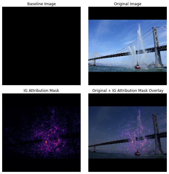"},{"metadata":{"papermill":{"duration":0.042459,"end_time":"2021-01-13T22:39:39.678624","exception":false,"start_time":"2021-01-13T22:39:39.636165","status":"completed"},"tags":[]},"cell_type":"markdown","source":"3 NOTEBOOK SETUP"},{"metadata":{"execution":{"iopub.execute_input":"2021-01-13T22:39:39.779248Z","iopub.status.busy":"2021-01-13T22:39:39.778548Z","iopub.status.idle":"2021-01-13T22:39:40.76653Z","shell.execute_reply":"2021-01-13T22:39:40.767021Z"},"papermill":{"duration":1.046203,"end_time":"2021-01-13T22:39:40.767178","exception":false,"start_time":"2021-01-13T22:39:39.720975","status":"completed"},"tags":[],"trusted":true},"cell_type":"code","source":"# Define the root data directory\nTRAIN_IMG_DIR = KaggleDatasets().get_gcs_path(\"hpa-512512\")\nLOCAL_DATA_DIR = \"/kaggle/input/hpa-single-cell-image-classification\"\n\n# Capture all the relevant full image paths\nTRAIN_IMG_PATHS = tf.io.gfile.glob(os.path.join(TRAIN_IMG_DIR, '*.png'))\nMODEL_DIR = \"/kaggle/input/hpa-xai-ig-tfrecords-tpu-training/model\"\n\n# Capture all the relevant full image paths\nTRAIN_IMG_PATHS = tf.io.gfile.glob(os.path.join(TRAIN_IMG_DIR, '*.png'))\n\nprint(f\"\\n... Recall that 4 training images compose one example (R,G,B,Y) ...\")\nprint(f\"... \\t– i.e. The first 4 training files are:\")\nfor path in [x.rsplit('/',1)[1] for x in TRAIN_IMG_PATHS[:4]]: print(f\"... \\t\\t– {path}\")\nprint(f\"\\n... The number of training images is {len(TRAIN_IMG_PATHS)} i.e. {len(TRAIN_IMG_PATHS)//4} 4-channel images ...\")\n\n# Define paths to the relevant csv files &\n# create the relevant dataframe objects\nTRAIN_CSV = os.path.join(LOCAL_DATA_DIR, \"train.csv\")\ntrain_df = pd.read_csv(TRAIN_CSV)\nprint(\"\\n\\nTRAIN DATAFRAME\\n\\n\")\ndisplay(train_df.head(3))\n\nSS_CSV = os.path.join(LOCAL_DATA_DIR, \"sample_submission.csv\")\nss_df = pd.read_csv(SS_CSV)\nprint(\"\\n\\nSAMPLE SUBMISSION DATAFRAME\\n\\n\")\ndisplay(ss_df.head(3))\n\n# Create Various-Label-Count Dataframes\ndfs_by_label_cnt = {(i+1):train_df[train_df.Label.str.count(\"\\|\")==i].reset_index(drop=True) for i in range(5)}\ndisplay(dfs_by_label_cnt[1].head(3))\ndisplay(dfs_by_label_cnt[2].head(3))\ndisplay(dfs_by_label_cnt[3].head(3))\ndisplay(dfs_by_label_cnt[4].head(3))\ndisplay(dfs_by_label_cnt[5].head(3))","execution_count":null,"outputs":[]},{"metadata":{"papermill":{"duration":0.043842,"end_time":"2021-01-13T22:39:40.85577","exception":false,"start_time":"2021-01-13T22:39:40.811928","status":"completed"},"tags":[]},"cell_type":"markdown","source":"4 HELPER FUNCTIONS"},{"metadata":{"_cell_guid":"79c7e3d0-c299-4dcb-8224-4455121ee9b0","_uuid":"d629ff2d2480ee46fbb7e2d37f6b5fab8052498a","execution":{"iopub.execute_input":"2021-01-13T22:39:40.980411Z","iopub.status.busy":"2021-01-13T22:39:40.979421Z","iopub.status.idle":"2021-01-13T22:39:40.982404Z","shell.execute_reply":"2021-01-13T22:39:40.981881Z"},"papermill":{"duration":0.080032,"end_time":"2021-01-13T22:39:40.982523","exception":false,"start_time":"2021-01-13T22:39:40.902491","status":"completed"},"tags":[],"trusted":true},"cell_type":"code","source":"def decode_img(image_data, resize_to=(512,512)):\n image = tf.image.decode_png(image_data, channels=1)\n # explicit size needed for TPU\n image = tf.reshape(image, resize_to) \n return tf.cast(image, tf.float32)\n\n\ndef load_image(img_id, img_dir, resize_to=(512,512), tpu_style=False):\n \"\"\" Load An Image Using ID and Directory Path - Composes 4 Individual Images \"\"\"\n if not tpu_style:\n rgby = [\n np.asarray(Image.open(os.path.join(img_dir, img_id+f\"_{c}.png\")).resize(resize_to), np.uint8) \\\n for c in [\"red\", \"green\", \"blue\", \"yellow\"]\n ]\n return np.stack(rgby, axis=-1)\n else:\n rgby = [\n decode_img(tf.io.read_file(os.path.join(img_dir, img_id+f\"_{c}.png\")), resize_to) \\\n for c in [\"red\", \"green\", \"blue\", \"yellow\"]\n ]\n return tf.stack(rgby, axis=-1)\n\ndef plot_rgb(arr, figsize=(12,12)):\n \"\"\" Plot 3 Channel Microscopy Image \"\"\"\n plt.figure(figsize=figsize)\n plt.title(f\"RGB Composite Image\", fontweight=\"bold\")\n plt.imshow(arr)\n plt.axis(False)\n plt.show()\n \n \ndef convert_rgby_to_rgb(arr, boost_green=False):\n \"\"\" Convert a 4 channel (RGBY) image to a 3 channel RGB image.\n \n Advice From Competition Host/User: lnhtrang\n\n For annotation (by experts) and for the model, I guess we agree that individual \n channels with full range px values are better. \n In annotation, we toggled the channels. \n For visualization purpose only, you can try blending the channels. \n For example, \n - red = red + yellow\n - green = green + yellow/2\n - blue=blue.\n \n Args:\n arr (numpy array): The RGBY, 4 channel numpy array for a given image\n boost_green (numpy array): Whether to boost the intensity of the green channel\n \n Returns:\n RGB Image\n \"\"\"\n \n rgb_arr = np.zeros_like(arr[..., :-1])\n if boost_green:\n rgb_arr[..., 0] = arr[..., 0]/1.25\n rgb_arr[..., 1] = np.clip(arr[..., 1]*2+arr[..., 3]/5, 0, 255)\n rgb_arr[..., 2] = arr[..., 2]/1.25\n rgb_arr = rgb_arr.astype(np.uint8)\n else:\n rgb_arr[..., 0] = arr[..., 0]\n rgb_arr[..., 1] = arr[..., 1]+arr[..., 3]/2\n rgb_arr[..., 2] = arr[..., 2]\n \n return rgb_arr\n\n\n\ndef plot_ex(arr, figsize=(20,6), title=None, plot_merged=True, rgb_only=False):\n \"\"\" Plot 4 Channels Side by Side \"\"\"\n if plot_merged and not rgb_only:\n n_images=5 \n elif plot_merged and rgb_only:\n n_images=4\n elif plot_merged and rgb_only:\n n_images=4\n else:\n n_images=3\n plt.figure(figsize=figsize)\n if type(title) == str:\n plt.suptitle(title, fontsize=20, fontweight=\"bold\")\n\n for i, c in enumerate([\"Red Channel – Microtubles\", \"Green Channel – Protein of Interest\", \"Blue - Nucleus\", \"Yellow – Endoplasmic Reticulum\"]):\n if not rgb_only:\n ch_arr = np.zeros_like(arr[..., :-1]) \n else:\n ch_arr = np.zeros_like(arr)\n if c in [\"Red Channel – Microtubles\", \"Green Channel – Protein of Interest\", \"Blue - Nucleus\"]:\n ch_arr[..., i] = arr[..., i]\n else:\n if rgb_only:\n continue\n ch_arr[..., 0] = arr[..., i]\n ch_arr[..., 1] = arr[..., i]\n plt.subplot(1,n_images,i+1)\n plt.title(f\"{c.title()}\", fontweight=\"bold\")\n plt.imshow(ch_arr)\n plt.axis(False)\n \n if plot_merged:\n plt.subplot(1,n_images,n_images)\n \n if rgb_only:\n plt.title(f\"Merged RGB\", fontweight=\"bold\")\n plt.imshow(arr)\n else:\n plt.title(f\"Merged RGBY into RGB\", fontweight=\"bold\")\n plt.imshow(convert_rgby_to_rgb(arr))\n plt.axis(False)\n \n plt.tight_layout(rect=[0, 0.2, 1, 0.97])\n plt.show()\n \n \ndef flatten_list_of_lists(l_o_l):\n return [item for sublist in l_o_l for item in sublist]\n\n\ndef load_batch_of_images(df, id_list, img_dir, resize_to=(512,512), return_labels=True, tpu_style=False):\n if not return_labels:\n return np.stack([load_image(ID, img_dir, resize_to) for ID in id_list], axis=0)\n else:\n lbls = df[df.ID.isin(id_list)].Label.apply(lambda x: [int(l) for l in x.split(\"|\")]).to_list()\n return np.stack([load_image(ID, img_dir, resize_to, tpu_style=tpu_style) for ID in id_list], axis=0), lbls\n \ndef plot_batch_of_images(img_batch, lbl_batch=None, pred_batch=None, n_cols=4, labels_as_strs=True, boost_green=True):\n n_imgs = img_batch.shape[0]\n if not lbl_batch:\n lbl_batch = [None,]*n_imgs\n if not pred_batch:\n pred_batch = [None,]*n_imgs\n \n plt.figure(figsize=(19, int(5.5*np.ceil(n_imgs/n_cols))))\n for i, (img, lbl, pred) in enumerate(zip(img_batch, lbl_batch, pred_batch)):\n plt.subplot(int(np.ceil(n_imgs/n_cols)), n_cols, i+1)\n if lbl or pred:\n title_str = \"\"\n if lbl:\n if labels_as_strs:\n title_str+=f\"GT LABEL: {[INT_2_STR[l] for l in lbl]}\"\n else:\n title_str+=f\"GT LABEL: {sorted(list(lbl))}\"\n if pred:\n if labels_as_strs:\n title_str+=f\"\\nPRED LABEL: {[INT_2_STR[p] for p in pred[0]]}\"\n else:\n title_str+=f\"\\nPRED LABEL: {sorted(list(pred[0]))}\"\n plt.title(title_str.strip(\"\\n\"), fontweight=\"bold\")\n plt.imshow(convert_rgby_to_rgb(img, boost_green=boost_green))\n plt.axis(False)\n\n plt.tight_layout()\n plt.show()\n \ndef get_pred(model, img_batch, conf_thresh=0.3, drop_yellow=True):\n if drop_yellow:\n img_batch = img_batch[..., :-1]\n pred_batch = model.predict(img_batch)\n return [np.where(p>conf_thresh) for p in pred_batch]\n\ndef interpolate_images(baseline, image, alphas=None):\n if alphas is None:\n alphas = tf.linspace(start=0.0, stop=1.0, num=25)\n\n # type coercion\n _image = tf.cast(image, alphas.dtype)\n _baseline = tf.cast(baseline, alphas.dtype)\n \n if tf.math.reduce_max(_image)>1.:\n _image /= 255.\n \n if tf.math.reduce_max(_baseline)>1.:\n _baseline /= 255.\n \n # Give alphas, baseline, and input all 4 dimensions (b, w, h, c)\n alphas_x = alphas[:, tf.newaxis, tf.newaxis, tf.newaxis]\n baseline_x = tf.expand_dims(_baseline, axis=0)\n \n input_x = tf.expand_dims(_image, axis=0)\n \n # Calculate delta\n delta = input_x - baseline_x\n\n # Create the stepwise images between baseline and the original image\n # As alphas_x increases the contribution of the original image \n # (represented by delta in our case) grows to become the original value\n #\n # This is in essence, stepping from pure black towards the original\n images = baseline_x + alphas_x*delta\n return images*255\n\ndef compute_gradients(model, images, target_class_idx):\n if images.dtype != tf.float32:\n images = tf.cast(images, tf.float32)\n \n if tf.math.reduce_max(images)<=1.:\n images *= 255.\n \n with tf.GradientTape() as tape:\n tape.watch(images)\n target_pred = model(images)[:, target_class_idx]\n \n return tape.gradient(target_pred, images)\n\ndef integral_approximation(gradients):\n # riemann_trapezoidal\n grads = (gradients[:-1] + gradients[1:]) / tf.constant(2.0)\n integrated_gradients = tf.math.reduce_mean(grads, axis=0)\n return integrated_gradients\n\ndef process_attributions(attributions, rescale_power=1, grayscale=False):\n def _min_max_tensor(tensor, exp=1):\n return tf.math.divide(tf.subtract(tensor, tf.reduce_min(tensor)), \n tf.subtract(tf.reduce_max(tensor), tf.reduce_min(tensor)))**exp\n \n pos_attribution_mask = \\\n tf.reduce_sum(tf.math.abs(tf.clip_by_value(attributions, 0, 10000)), axis=-1)\n neg_attribution_mask = \\\n tf.reduce_sum(tf.math.abs(tf.clip_by_value(attributions, -10000, 0)), axis=-1)\n\n pos_attribution_mask = _min_max_tensor(pos_attribution_mask, 1/rescale_power)\n neg_attribution_mask = _min_max_tensor(neg_attribution_mask, 1/rescale_power)\n \n if grayscale:\n return tf.clip_by_value(pos_attribution_mask+neg_attribution_mask, 0.0, 1.0)\n else:\n return pos_attribution_mask, neg_attribution_mask\n\ndef make_attribution_cmap():\n # Make special colour maps\n pos_cmap = sns.dark_palette(\"red\")\n pos_cmap.insert(0, (0.,0.,0.))\n pos_cmap = ListedColormap(pos_cmap)\n\n neg_cmap = sns.dark_palette(\"blue\")\n neg_cmap.insert(0, (0.,0.,0.))\n neg_cmap = ListedColormap(neg_cmap)\n\n return pos_cmap, neg_cmap\n\ndef plot_img_attributions(attributions, baseline, image, class_label, overlay_alpha=0.5, save_fig=True, rescale_power=1): \n pos_cmap, neg_cmap = make_attribution_cmap()\n\n # Sum of the attributions across color channels for visualization.\n # The attribution mask shape is a grayscale image with height and width\n # equal to the original image.\n pos_attribution_mask, neg_attribution_mask = process_attributions(attributions, rescale_power)\n \n combined_masks = np.zeros_like(attributions)\n combined_masks[:, :, 0] = pos_attribution_mask\n combined_masks[:, :, 2] = neg_attribution_mask\n\n # Plotting\n plt.figure(figsize=(19,16))\n\n plt.suptitle(\"Attribution Visualization for the {} Class\\n\\n\\n\" \\\n \"\".format(class_label), fontsize=16, fontweight=\"bold\")\n \n plt.subplot(2,3,1)\n plt.title('\\nBaseline image', fontweight=\"bold\")\n plt.imshow(baseline)\n plt.axis('off')\n \n plt.subplot(2,3,2)\n plt.title('\\nPositive Attribution Mask', fontweight=\"bold\")\n plt.imshow(pos_attribution_mask, cmap=pos_cmap)\n plt.axis('off')\n\n plt.subplot(2,3,3)\n plt.title('\\nNegative Attribution Mask', fontweight=\"bold\")\n plt.imshow(neg_attribution_mask, cmap=neg_cmap)\n plt.axis('off')\n\n plt.subplot(2,3,4)\n plt.title('Original image', fontweight=\"bold\")\n plt.imshow(image/255)\n plt.axis('off')\n\n plt.subplot(2,3,5)\n plt.title('Full Attribution mask', fontweight=\"bold\")\n plt.imshow(combined_masks)\n plt.axis('off')\n\n plt.subplot(2,3,6)\n plt.title('Overlay', fontweight=\"bold\")\n # plt.imshow(np.sum(combined_masks, axis=2), cmap=\"gray\")\n plt.imshow(combined_masks)\n plt.imshow(image/255, alpha=overlay_alpha)\n plt.axis('off')\n \n if save_fig:\n plt.savefig(f\"/kaggle/working/{c}.jpg\" ,dpi=400)\n \n plt.tight_layout()\n plt.show()\n \n return combined_masks\n\n@tf.function(experimental_relax_shapes=False)\ndef integrated_gradients(model, \n baseline,\n image,\n target_class_idx,\n m_steps=64,\n batch_size=8):\n \n\n # Step 0. Format Check\n if tf.math.reduce_max(image)<=1.:\n image *= 255.\n if tf.math.reduce_max(baseline)<=1.:\n baseline *= 255.\n \n # Step 1. Generate alphas\n alphas = tf.linspace(start=tf.constant(0, dtype=tf.float32), \n stop=tf.constant(1, dtype=tf.float32), \n num=m_steps)\n\n # Accumulate gradients across batches\n integrated_gradients = 0.0\n\n # Batch alpha images\n ds = tf.data.Dataset.from_tensor_slices(alphas).batch(batch_size)\n\n for batch in ds:\n # Step 2. Generate interpolated images\n batch_interpolated_inputs = interpolate_images(baseline=baseline/255,\n image=image/255,\n alphas=batch)\n\n # Step 3. Compute gradients between model outputs and interpolated inputs\n batch_gradients = compute_gradients(model,\n images=batch_interpolated_inputs,\n target_class_idx=target_class_idx)\n\n # Step 4. Average integral approximation. Summing integrated gradients across batches.\n integrated_gradients += integral_approximation(gradients=batch_gradients)\n\n # Step 5. Scale integrated gradients with respect to input\n scaled_integrated_gradients = (image - baseline) * integrated_gradients\n return scaled_integrated_gradients\n\ndef get_labels_from_id(target_id, df):\n return [int(x) for x in df[df.ID==target_id].Label.str.split(\"|\").to_list()[0]]","execution_count":null,"outputs":[]},{"metadata":{},"cell_type":"markdown","source":"5 LOAD AND DEMONSTRATE MODEL PREDICTION"},{"metadata":{},"cell_type":"markdown","source":"5.1 LOAD THE TRAINED MODEL
\n\n---"},{"metadata":{"trusted":true},"cell_type":"code","source":"with strategy.scope():\n load_locally = tf.saved_model.LoadOptions(experimental_io_device='/job:localhost')\n enet = tf.keras.models.load_model(MODEL_DIR, options=load_locally) # loading in Tensorflow's \"SavedModel\" format","execution_count":null,"outputs":[]},{"metadata":{},"cell_type":"markdown","source":"5.2 SHOW MODEL PREDICTIONS
\n\n---\n\n- Grab a random batch of single label IDs\n- Get images and labels for batch from each label-count dataframe\n- Get predictions for batch at a given confidence threshold\n- Visualize"},{"metadata":{"trusted":true},"cell_type":"code","source":"DEMO_BATCH_SIZE = 4\n\nfor i in range(1, 6):\n if i==5:\n DEMO_BATCH_SIZE=len(dfs_by_label_cnt[i])\n print(f\"\\n... {DEMO_BATCH_SIZE} PREDICTIONS FOR IMAGES WITH {i} LABELS ...\\n\")\n RNDM_SNGL_LBL_IDS = dfs_by_label_cnt[i].ID.sample(DEMO_BATCH_SIZE).sort_index().to_list()\n print(RNDM_SNGL_LBL_IDS)\n img_batch, lbl_batch = load_batch_of_images(dfs_by_label_cnt[i], RNDM_SNGL_LBL_IDS, TRAIN_IMG_DIR, tpu_style=True)\n pred_batch = get_pred(enet, img_batch, conf_thresh=0.225, drop_yellow=True)\n plot_batch_of_images(img_batch, lbl_batch, pred_batch, n_cols=4, labels_as_strs=False, boost_green=True)","execution_count":null,"outputs":[]},{"metadata":{},"cell_type":"markdown","source":"5.3 SHOW INTEGRATED GRADIENTS ON A DIFFICULT, MULTI-LABEL IMAGE
\n\n---\n\n- Calculate IG For The Same Image Monitoring Each GT Label Respectively\n- Preprocess These Attributions To Improve Visability (Rescale Between 0-1 and Raise to Fractional Power)\n- Visualize"},{"metadata":{"trusted":true},"cell_type":"code","source":"IG_IMG_ID = \"8e998b50-bbb0-11e8-b2ba-ac1f6b6435d0\"\nBASELINE = tf.zeros(shape=(512,512,3), dtype=tf.float32)\nIG_IMG = tf.cast(load_image(IG_IMG_ID, TRAIN_IMG_DIR, tpu_style=True), tf.float32)\nIG_LBLS = get_labels_from_id(IG_IMG_ID, train_df)\nCMAP=\"magma\"\n\nIG_LBL_MAP = {\n l:integrated_gradients(enet, \n BASELINE,\n image=IG_IMG[..., :-1], \n target_class_idx=tf.constant(l)) \\\n for l in tqdm(IG_LBLS)}","execution_count":null,"outputs":[]},{"metadata":{"trusted":true},"cell_type":"code","source":"attr_img = np.zeros((512,512,len(IG_LBL_MAP)))\nplt.figure(figsize=(20,16))\nfor i, (cls,ig_attr) in enumerate(IG_LBL_MAP.items()):\n attr = process_attributions(ig_attr, rescale_power=tf.constant(1.4, dtype=tf.float32), grayscale=True)\n plt.subplot(2,int(np.ceil((len(IG_LBL_MAP)+1)/2)),i+1)\n plt.imshow(attr, cmap=CMAP)\n plt.title(f\"{INT_2_STR[cls]} Attribution Map\", fontweight=\"bold\")\n plt.axis(False)\n\n# Show the ground truth image \nplt.subplot(2,int(np.ceil((len(IG_LBL_MAP)+1)/2)),len(IG_LBL_MAP)+1)\nplt.imshow(convert_rgby_to_rgb(IG_IMG.numpy(), boost_green=True))\nplt.title(\"Image With Green Channel Boosted\", fontweight=\"bold\")\nplt.axis(False)\n\nplt.tight_layout()\nplt.savefig(\"demonstration_ig.png\", dpi=600)\nplt.show()","execution_count":null,"outputs":[]},{"metadata":{"trusted":true},"cell_type":"code","source":"","execution_count":null,"outputs":[]}],"metadata":{"kernelspec":{"language":"python","display_name":"Python 3","name":"python3"},"language_info":{"pygments_lexer":"ipython3","nbconvert_exporter":"python","version":"3.6.4","file_extension":".py","codemirror_mode":{"name":"ipython","version":3},"name":"python","mimetype":"text/x-python"}},"nbformat":4,"nbformat_minor":4}