
First of all, we would like to express our gratitude to the staff and Kagglers who shared great information and knowledge. We are thrilled to say that by winning the gold medal in this competition, four members from our team have achieved the Kaggle Competitions Master.
\nWe merged Japanese team (Occccn, ktokunaga) and Irish team (Aindriú, RehanAhmed, Rishubh Khurana) right before the deadline for team merging. The Japanese team prepared a 2D model using spectrogram images and a 2D 1D combo model using both spectrogram images and raw EEG data. The Irish team prepared a 1D model, and also 2D 1D combo model. Upon Aindriú's suggestion, we used the geometric mean to merge the predictions.
\nIn this solution, we will focus only on the solution from the Japanese team.
\nWe adopted a two-stage learning strategy, initially training on data with less than <10 labels and then further training on data with ≥10 labels. After the first round of training, we replaced the origianl labels for <10 labels data with the model's predicted labels, treating them as pseudo labels for a second round of training. Using pseudo labels confirmed improvements in the LB scores.
\nAs mentioned in this discussion, we speculate that Training Dataset3 in the image below corresponds to the data in train.csv with ≥10 labels. Further scrutiny revealed that the train.csv data with ≥10 labels contained a higher proportion of 'Other' labels compared to Training Dataset3. We hypothesized that some of the 'Other' labeled data from train.csv with ≥10 labels may be inaccurately labeled by insufficiently trained physicians. Assuming that Test Dataset4 corresponds to Kaggle's test dataset, such inaccurately labeld data are not included in the test dataset. Therefore, training on the train.csv data with ≥10 labels would inadvertently tune the model to expect a higher ratio of 'Other' labels than is present in the test dataset.
\n
As a result, we decided not to use some of the 'Other' data with >10 labels in the second stage of learning. As an another method, following advice from Aindriú, we applied a postprocessing step to adjust the 'Other' prediction values by raising them to the power of 1.1 after merging predictions of ensemble models. This postprocessing confirmed improvements in LB scores.
\npred[:,] = pred[:,]**\npred = pred/pred.(axis=,keepdims=)\nExperiments showed that spectrograms transformed using CWT were more effective than those using STFT. Following a similar approach to Chris's excellent Notebook, we took differences and changed the transformation method to CWT. By converting to a 64-dimensional image in the frequency scale direction, we obtained spectrograms of 50 seconds in the size of (64, 10000, 4). We resized the first 20 seconds to (64, 512, 4), the middle 10 seconds to (64, 512, 4), and the last 10 seconds to (64, 512, 4), stacking them to create an image of (768, 512,1). This was connected to the 10-minute spectrograms provided by Kaggle to form the shape of (512, 1024, 1), which is then repeated to (512, 1024, 3) for image models like EfficientNet.
\nLL Spec = ( CWT(Fp1 - F7) + CWT(F7 - T3) + CWT(T3 - T5) + CWT(T5 - O1) ) / \nLP Spec = ( CWT(Fp1 - F3) + CWT(F3 - C3) + CWT(C3 - P3) + CWT(P3 - O1) ) / \nRP Spec = ( CWT(Fp2 - F4) + CWT(F4 - C4) + CWT(C4 - P4) + CWT(P4 - O2) ) / \nRL Spec = ( CWT(Fp2 - F8) + CWT(F8 - T4) + CWT(T4 - T6) + CWT(T6 - O2) ) / \nThe best public LB score 0.264 (private 0.313) by single model was achieved with the mexh wavelet, efficientnet_b2 model and the aforementioned pseudo labels. Additionally, for ensemble purposes, we also created model with the cmor wavelet, efficientnet_b0, and so on.
\nWe created models that combine spectrogram images with raw EEGs. The basic idea is to treat raw EEGs as 2D images, so we converted raw EEGs into 2D images using a 1D CNN. The conversion method is as follows.
\nWe concatenated this 1D CNN features and the CWT spectrograms (middle 10 seconds) and got features for combo models
\nThe best public LB score 0.266 (private 0.331) by single model was achieved with the mexh wavelet,the cmor wavelet, efficientnet_b0 model and the aforementioned pseudo labels.
\nFor ensemble purposes, we also created various model(efficientb0/2,only mexh etc.)
\narchitecture summary
\n
First of all, we would like to express our gratitude to the staff and Kagglers who shared great information and knowledge. We are thrilled to say that by winning the gold medal in this competition, four members from our team have achieved the Kaggle Competitions Master.
\nWe merged Japanese team (Occccn, ktokunaga) and Irish team (Aindriú, RehanAhmed, Rishubh Khurana) right before the deadline for team merging. The Japanese team prepared a 2D model using spectrogram images and a 2D 1D combo model using both spectrogram images and raw EEG data. The Irish team prepared a 1D model, and also 2D 1D combo model. Upon Aindriú's suggestion, we used the geometric mean to merge the predictions.
\nIn this solution, we will focus only on the solution from the Japanese team.
\nWe adopted a two-stage learning strategy, initially training on data with less than <10 labels and then further training on data with ≥10 labels. After the first round of training, we replaced the origianl labels for <10 labels data with the model's predicted labels, treating them as pseudo labels for a second round of training. Using pseudo labels confirmed improvements in the LB scores.
\nAs mentioned in this discussion, we speculate that Training Dataset3 in the image below corresponds to the data in train.csv with ≥10 labels. Further scrutiny revealed that the train.csv data with ≥10 labels contained a higher proportion of 'Other' labels compared to Training Dataset3. We hypothesized that some of the 'Other' labeled data from train.csv with ≥10 labels may be inaccurately labeled by insufficiently trained physicians. Assuming that Test Dataset4 corresponds to Kaggle's test dataset, such inaccurately labeld data are not included in the test dataset. Therefore, training on the train.csv data with ≥10 labels would inadvertently tune the model to expect a higher ratio of 'Other' labels than is present in the test dataset.
\n
As a result, we decided not to use some of the 'Other' data with >10 labels in the second stage of learning. As an another method, following advice from Aindriú, we applied a postprocessing step to adjust the 'Other' prediction values by raising them to the power of 1.1 after merging predictions of ensemble models. This postprocessing confirmed improvements in LB scores.
\npred[:,] = pred[:,]**\npred = pred/pred.(axis=,keepdims=)\nExperiments showed that spectrograms transformed using CWT were more effective than those using STFT. Following a similar approach to Chris's excellent Notebook, we took differences and changed the transformation method to CWT. By converting to a 64-dimensional image in the frequency scale direction, we obtained spectrograms of 50 seconds in the size of (64, 10000, 4). We resized the first 20 seconds to (64, 512, 4), the middle 10 seconds to (64, 512, 4), and the last 10 seconds to (64, 512, 4), stacking them to create an image of (768, 512,1). This was connected to the 10-minute spectrograms provided by Kaggle to form the shape of (512, 1024, 1), which is then repeated to (512, 1024, 3) for image models like EfficientNet.
\nLL Spec = ( CWT(Fp1 - F7) + CWT(F7 - T3) + CWT(T3 - T5) + CWT(T5 - O1) ) / \nLP Spec = ( CWT(Fp1 - F3) + CWT(F3 - C3) + CWT(C3 - P3) + CWT(P3 - O1) ) / \nRP Spec = ( CWT(Fp2 - F4) + CWT(F4 - C4) + CWT(C4 - P4) + CWT(P4 - O2) ) / \nRL Spec = ( CWT(Fp2 - F8) + CWT(F8 - T4) + CWT(T4 - T6) + CWT(T6 - O2) ) / \nThe best public LB score 0.264 (private 0.313) by single model was achieved with the mexh wavelet, efficientnet_b2 model and the aforementioned pseudo labels. Additionally, for ensemble purposes, we also created model with the cmor wavelet, efficientnet_b0, and so on.
\nWe created models that combine spectrogram images with raw EEGs. The basic idea is to treat raw EEGs as 2D images, so we converted raw EEGs into 2D images using a 1D CNN. The conversion method is as follows.
\nWe concatenated this 1D CNN features and the CWT spectrograms (middle 10 seconds) and got features for combo models
\nThe best public LB score 0.266 (private 0.331) by single model was achieved with the mexh wavelet,the cmor wavelet, efficientnet_b0 model and the aforementioned pseudo labels.
\nFor ensemble purposes, we also created various model(efficientb0/2,only mexh etc.)
\narchitecture summary
\n
Congratulations on Gold medal finish!
\nI am confused. If the following is true, shouldn't we multiply Other by a number less than 1 like 0.9? Why do you multiply by 1.1?
\n\nTherefore, training on the train.csv data with ≥10 labels would inadvertently tune the model to expect a higher ratio of 'Other' labels than is present in the test dataset.
\n
Here is your post process:
\n\n", "rawMarkdown": "Congratulations on Gold medal finish!\n\nI am confused. If the following is true, shouldn't we multiply `Other` by a number less than 1 like `0.9`? Why do you multiply by `1.1`?\n\n>Therefore, training on the train.csv data with ≥10 labels would inadvertently tune the model to expect a higher ratio of 'Other' labels than is present in the test dataset.\n\nHere is your post process:\n\n>pred[:,5] = pred[:,5]**1.1\npred = pred/pred.sum(axis=1,keepdims=True)", "votes": null }, { "id": "2750131", "postDate": "04/13/2024 13:18:05", "content": "pred[:,5] = pred[:,5]**1.1
\n
\n pred = pred/pred.sum(axis=1,keepdims=True)
Thank you for your comment!
\nSorry for the complication. It's the power, not the multiplication. Raising a probability to the power of 1.1 will get a smaller value.
Thanks for explanation. Congratulations on 14th place ! 🔥
", "rawMarkdown": "Thanks for explanation. Congratulations on 14th place ! 🔥", "votes": null } ], "comments": [ { "id": 2749078, "author_name": "cdeotte", "author_url": "", "post_date": "04/12/2024 20:13:00", "content": "Congratulations on Gold medal finish!
\nI am confused. If the following is true, shouldn't we multiply Other by a number less than 1 like 0.9? Why do you multiply by 1.1?
\n\nTherefore, training on the train.csv data with ≥10 labels would inadvertently tune the model to expect a higher ratio of 'Other' labels than is present in the test dataset.
\n
Here is your post process:
\n\n", "votes": null, "replies": [ { "id": 2750131, "author_name": "kazuakitokunaga", "author_url": "", "post_date": "04/13/2024 13:18:05", "content": "pred[:,5] = pred[:,5]**1.1
\n
\n pred = pred/pred.sum(axis=1,keepdims=True)
Thank you for your comment!
\nSorry for the complication. It's the power, not the multiplication. Raising a probability to the power of 1.1 will get a smaller value.
Thanks for explanation. Congratulations on 14th place ! 🔥
", "votes": null, "replies": [] } ], "raw_markdown_by_id": { "2747812": "First of all, we would like to express our gratitude to the staff and Kagglers who shared great information and knowledge. We are thrilled to say that by winning the gold medal in this competition, four members from our team have achieved the Kaggle Competitions Master.\n\n# Summary\n\nWe merged Japanese team (Occccn, ktokunaga) and Irish team (Aindriú, RehanAhmed, Rishubh Khurana) right before the deadline for team merging. The Japanese team prepared a 2D model using spectrogram images and a 2D 1D combo model using both spectrogram images and raw EEG data. The Irish team prepared a 1D model, and also 2D 1D combo model. Upon Aindriú's suggestion, we used the geometric mean to merge the predictions.\n\nIn this solution, we will focus only on the solution from the Japanese team.\n\n# Japanese team solution\n\n### Learning Strategy\n\nWe adopted a two-stage learning strategy, initially training on data with less than <10 labels and then further training on data with ≥10 labels. After the first round of training, we replaced the origianl labels for <10 labels data with the model's predicted labels, treating them as pseudo labels for a second round of training. Using pseudo labels confirmed improvements in the LB scores.\n\n### About Test Dataset\n\nAs mentioned in [this discussion](https://www.kaggle.com/competitions/hms-harmful-brain-activity-classification/discussion/492262), we speculate that Training Dataset3 in the image below corresponds to the data in train.csv with ≥10 labels. Further scrutiny revealed that the train.csv data with ≥10 labels contained a higher proportion of 'Other' labels compared to Training Dataset3. We hypothesized that some of the 'Other' labeled data from train.csv with ≥10 labels may be inaccurately labeled by insufficiently trained physicians. Assuming that Test Dataset4 corresponds to Kaggle's test dataset, such inaccurately labeld data are not included in the test dataset. Therefore, training on the train.csv data with ≥10 labels would inadvertently tune the model to expect a higher ratio of 'Other' labels than is present in the test dataset.\n\n\n\nAs a result, we decided not to use some of the 'Other' data with >10 labels in the second stage of learning. As an another method, following advice from Aindriú, we applied a postprocessing step to adjust the 'Other' prediction values by raising them to the power of 1.1 after merging predictions of ensemble models. This postprocessing confirmed improvements in LB scores.\n\n```python\npred[:,5] = pred[:,5]**1.1\npred = pred/pred.sum(axis=1,keepdims=True)\n```\n\n### 2D model (mainly by ktokunaga)\n\nExperiments showed that spectrograms transformed using CWT were more effective than those using STFT. Following a similar approach to [Chris's excellent Notebook](https://www.kaggle.com/code/cdeotte/how-to-make-spectrogram-from-eeg), we took differences and changed the transformation method to CWT. By converting to a 64-dimensional image in the frequency scale direction, we obtained spectrograms of 50 seconds in the size of (64, 10000, 4). We resized the first 20 seconds to (64, 512, 4), the middle 10 seconds to (64, 512, 4), and the last 10 seconds to (64, 512, 4), stacking them to create an image of (768, 512,1). This was connected to the 10-minute spectrograms provided by Kaggle to form the shape of (512, 1024, 1), which is then repeated to (512, 1024, 3) for image models like EfficientNet.\n\n```python\nLL Spec = ( CWT(Fp1 - F7) + CWT(F7 - T3) + CWT(T3 - T5) + CWT(T5 - O1) ) / 4\nLP Spec = ( CWT(Fp1 - F3) + CWT(F3 - C3) + CWT(C3 - P3) + CWT(P3 - O1) ) / 4\nRP Spec = ( CWT(Fp2 - F4) + CWT(F4 - C4) + CWT(C4 - P4) + CWT(P4 - O2) ) / 4\nRL Spec = ( CWT(Fp2 - F8) + CWT(F8 - T4) + CWT(T4 - T6) + CWT(T6 - O2) ) / 4\n```\n\nThe best public LB score 0.264 (private 0.313) by single model was achieved with the mexh wavelet, efficientnet_b2 model and the aforementioned pseudo labels. Additionally, for ensemble purposes, we also created model with the cmor wavelet, efficientnet_b0, and so on.\n\n### 2D / 1D combo model (mainly by **Occccn**)\n\nWe created models that combine spectrogram images with raw EEGs. The basic idea is to treat raw EEGs as 2D images, so we converted raw EEGs into 2D images using a 1D CNN. The conversion method is as follows.\n\n1. Create a data of (24,2000) by taking the difference between various EEGs and downsampling.\n2. Convert (1,2000) by using multiple 1DCNN layers into a data of (64, 512), finally we get a data of (64,512,24).\n3. Reshape the (64,512,24) data into (512,512,3).\n\nWe concatenated this 1D CNN features and the CWT spectrograms (middle 10 seconds) and got features for combo models\n\nThe best public LB score 0.266 (private 0.331) by single model was achieved with the mexh wavelet,the cmor wavelet, efficientnet_b0 model and the aforementioned pseudo labels. \n\nFor ensemble purposes, we also created various model(efficientb0/2,only mexh etc.)\n\n**architecture summary**\n\n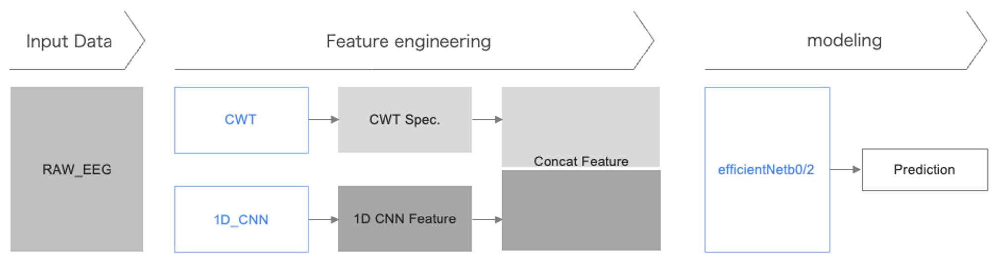\n\n### What doesn’t work for us\n\n- data augmentation (flipping, gaussian noise, etc.)\n- using external dataset", "2749078": "Congratulations on Gold medal finish!\n\nI am confused. If the following is true, shouldn't we multiply `Other` by a number less than 1 like `0.9`? Why do you multiply by `1.1`?\n\n>Therefore, training on the train.csv data with ≥10 labels would inadvertently tune the model to expect a higher ratio of 'Other' labels than is present in the test dataset.\n\nHere is your post process:\n\n>pred[:,5] = pred[:,5]**1.1\npred = pred/pred.sum(axis=1,keepdims=True)", "2750131": "Thank you for your comment!\nSorry for the complication. It's the power, not the multiplication. Raising a probability to the power of 1.1 will get a smaller value.", "2750322": "Thanks for explanation. Congratulations on 14th place ! 🔥" }, "source": "meta" }