{"cells":[{"metadata":{"_uuid":"99bc5558af8549c0945d380f1e1544f5979974bf"},"cell_type":"markdown","source":"# **Histopathologic Cancer Detection**\n\nIdentify metastatic tissue in histopathologic scans of lymph node sections. This problem is a **binary classification problem** in which the **evaluation metric is area under roc curve**.\n\n**CONTENT: **\n\n**1.** Introduction and understanding of the problem given\n\n![](http://)**2.** Understanding the evalution metric for the given problem\n\n**3.** Simple EDA - (Exploratory Data Analysis)\n\n**4.** Different Modeling Strategies\n\n**5.** Validation and Analysis of results\n\n**5.** Modeling Limitations/Constraints\n\n**6.** Final model submission file creation\n\n**7.** Scope for further imrpovement"},{"metadata":{"_uuid":"aa21559892e02b9a906b39093707066c69266962"},"cell_type":"markdown","source":"# **1. INTRODUCTION AND UNDERSTANDING THE GIVEN PROBLEM**\n\nIn this competition, we need to create an algorithm to identify metastatic cancer in small image patches taken from larger digital pathology scans. A **metastasis refers to the spread of cancer cells from their primary location (the organ in which the cancer began) to another region of the body**. Cancer cells may spread through the bloodstream, the lymphatic vessels, or locally, and can do so because chemicals that ordinarily keep cells where they belong in the body are absent. **Cancers can metastasize to nearly any regions of the body, but some of the more common sites are the bones, lungs, liver, and brain**. Symptoms are often related to the presence of cancer cells in the organ where they spread. The treatment of metastases can vary with the original cancer and the region to which it has spread. **Understanding metastases is a critical area of cancer research, as metastatic disease is responsible for roughly 90 percent of cancer deaths**\n\n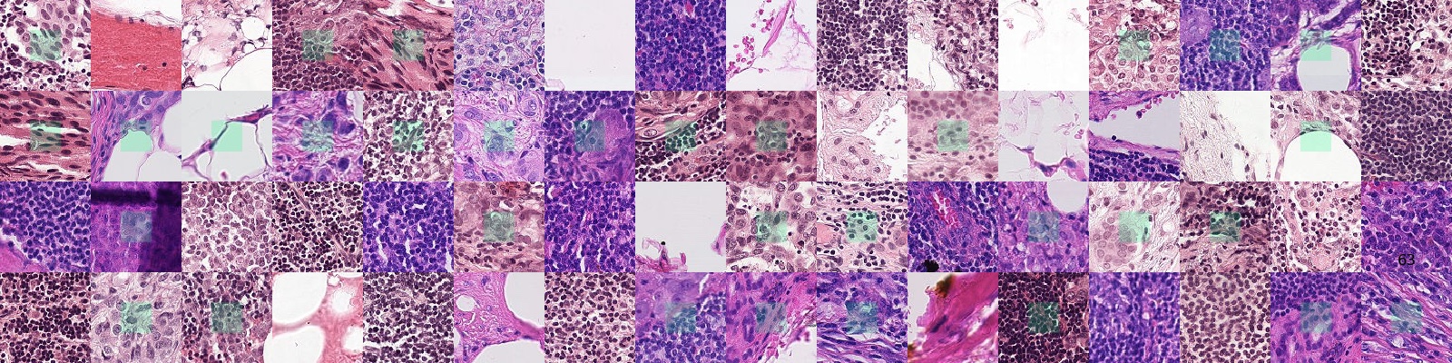![](https://raw.githubusercontent.com/basveeling/pcam/master/pcam.jpg).\n\nSo we are required to use our machine learning skills in order to create to reliable detector which might help saving many people life's by detecting cancer at early stages. "},{"metadata":{"_uuid":"9e2b4e1e6e23fb927babb293ee57ce0d95521ccd"},"cell_type":"markdown","source":"# **2. UNDERSTANDING THE EVALUTION METRIC OF THE GIVEN PROBLEM**\n\nAn **ROC curve** is a commonly used way to **visualize the performance of a binary classifier**, meaning a classifier with two possible output classes. Please open these links to get understanding of the metric:\n\n1. https://www.youtube.com/watch?v=OAl6eAyP-yo\n2. https://www.youtube.com/watch?v=xugjARegisk\n3. https://www.youtube.com/watch?v=egTNM8NSa2k\n\nVisit this link to get hands on experience on the ROC curve: http://www.navan.name/roc/\n\n"},{"metadata":{"_uuid":"73cb261d9bacfba1c7e70500902b98e488f2afda"},"cell_type":"markdown","source":"# **3. SIMPLE EDA  - (Exploratory Data Analysis)**"},{"metadata":{"_uuid":"8f2839f25d086af736a60e9eeb907d3b93b6e0e5","_cell_guid":"b1076dfc-b9ad-4769-8c92-a6c4dae69d19","trusted":true},"cell_type":"code","source":"# IMPORTING NECESSARY MODULES FOR DATA ANALYSIS AND PREDICTIVE MODELLING\nimport numpy as np\nimport pandas as pd\nimport seaborn as sns\nimport psutil\nimport cv2\nimport humanize\nfrom sklearn.preprocessing import LabelEncoder\nfrom sklearn.metrics import accuracy_score,confusion_matrix\nfrom sklearn.tree import DecisionTreeClassifier\nfrom sklearn.ensemble import RandomForestClassifier\nfrom sklearn.model_selection import train_test_split\nimport xgboost as xgb\nimport os\nimport gc\nfrom sklearn.model_selection import KFold, StratifiedKFold\nfrom tqdm import tqdm\nimport matplotlib.pyplot as plt\nfrom IPython.display import HTML, display, clear_output\nimport warnings\nwarnings.filterwarnings('ignore')\n%matplotlib inline\npd.set_option('display.max_rows', 500)\npd.set_option('display.max_columns', 500)","execution_count":null,"outputs":[]},{"metadata":{"trusted":true,"_uuid":"e897b70d102e63d1b7fe057d9368667023cddf31"},"cell_type":"code","source":"print(os.listdir('../input/'))","execution_count":null,"outputs":[]},{"metadata":{"_cell_guid":"79c7e3d0-c299-4dcb-8224-4455121ee9b0","_uuid":"d629ff2d2480ee46fbb7e2d37f6b5fab8052498a","trusted":true},"cell_type":"code","source":"#len(next(os.walk(\"../input/train/\"))[2]) # Number of images present in the train folder","execution_count":null,"outputs":[]},{"metadata":{"trusted":true,"_uuid":"f61251b92f7d0c88f89ef02fbf15b21087aa4666"},"cell_type":"code","source":"TrainDataPath = '../input/train_labels.csv'\nSubDataPath = '../input/sample_submission.csv'\n\n# Loading the Training and Test Dataset\nTrainData = pd.read_csv(TrainDataPath)\nSubData = pd.read_csv(SubDataPath)","execution_count":null,"outputs":[]},{"metadata":{"trusted":true,"_uuid":"4b38121b88fcc12e7abb9e31b38eb7f9f023a156"},"cell_type":"code","source":"print(\"Training Dataset Shape:\")\nprint(TrainData.shape)\nprint(\"\\n\")\nprint(\"Training Dataset Columns/Features:\")\nprint(TrainData.dtypes)\nTrainData.head()","execution_count":null,"outputs":[]},{"metadata":{"trusted":true,"_uuid":"3be0a6cfc1c177bb1ec06d609610855cf467498f"},"cell_type":"code","source":"# checking missing data percentage in train data\ntotal = TrainData.isnull().sum().sort_values(ascending = False)\npercent = (TrainData.isnull().sum()/TrainData.isnull().count()*100).sort_values(ascending = False)\nmissing_TrainData  = pd.concat([total, percent], axis=1, keys=['Total', 'Percent'])\nmissing_TrainData.head(10)","execution_count":null,"outputs":[]},{"metadata":{"trusted":true,"_uuid":"aa02ab55aad4af9722738439eadde1ef20103303"},"cell_type":"code","source":"SubData.head() # Submission Format","execution_count":null,"outputs":[]},{"metadata":{"_uuid":"78ee678ea4771b56c0373e0cdbb32451d494769c"},"cell_type":"markdown","source":"### Some Basic Stats Of The Dataset"},{"metadata":{"trusted":true,"_uuid":"cfba1f005e279a1f46a05fdf86ea7f3363681fe5"},"cell_type":"code","source":"print(\"Number Of Training Images Present In the Train Folder:\")\nprint(TrainData.shape[0])\nprint()\nprint(\"Number Of Test Images Present In the Test Folder:\")\nprint(SubData.shape[0])\nprint()\nprint()\nprint(\"0 - Represent Presence Of NO Tumors\")\nprint(\"1 - Represent Presence Of Tumors\")\nprint()\nprint()\nprint()\nprint(\"The Evaluation Metric For This Problem :  area under the ROC curve\")","execution_count":null,"outputs":[]},{"metadata":{"_uuid":"04c5be323504608fc46a17782e78410b11ad7f10"},"cell_type":"markdown","source":"# Helper Functions"},{"metadata":{"trusted":true,"_uuid":"b7cdf345010750bae857d47403309b7d404a4964"},"cell_type":"code","source":"def printmemusage():\n process = psutil.Process(os.getpid())\n print(\"Gen RAM Free: \" + humanize.naturalsize( psutil.virtual_memory().available ), \" | Proc size: \" + humanize.naturalsize( process.memory_info().rss))\nprintmemusage()","execution_count":null,"outputs":[]},{"metadata":{"trusted":true,"_uuid":"c744718d1562010c6ed336568c38fc4e1cc2df10"},"cell_type":"code","source":"# source: https://www.kaggle.com/gpreda/honey-bee-subspecies-classification\ndef draw_category_images(col_name,figure_cols, df, IMAGE_PATH):\n    categories = (df.groupby([col_name])[col_name].nunique()).index\n    f, ax = plt.subplots(nrows=len(categories),ncols=figure_cols, \n                         figsize=(4*figure_cols,4*len(categories))) # adjust size here\n    # draw a number of images for each location\n    for i, cat in enumerate(categories):\n        sample = df[df[col_name]==cat].sample(figure_cols) # figure_cols is also the sample size\n        for j in range(0,figure_cols):\n            file=IMAGE_PATH + sample.iloc[j]['id'] + '.tif'\n            im=cv2.imread(file)\n            ax[i, j].imshow(im, resample=True, cmap='gray')\n            ax[i, j].set_title('Label: '+str(cat), fontsize=16)  \n    plt.tight_layout()\n    plt.show()","execution_count":null,"outputs":[]},{"metadata":{"trusted":true,"_uuid":"99cc855ff70df914044e836dbf7fd7da8e3c78b5"},"cell_type":"code","source":"def train_test_data_check(train_df, test_df, cols=None, use_all_cols=True):\n    if cols == None:\n        if use_all_cols:\n            train_cols = set(train_df.columns)\n            test_cols = set(test_df.columns)\n            cols = train_cols.intersection(test_cols)\n        else:\n            train_cols = set(train_df.select_dtypes(['object', 'category']).columns)\n            test_cols = set(test_df.select_dtypes(['object', 'category']).columns)\n            cols = train_cols.intersection(test_cols)\n        \n    for i, col in enumerate(cols):\n        display(HTML('<h3><font id=\"'+ col + '-ttdc' + '\" color=\"blue\">' + str(i+1) + ') ' + col + '</font></h3>'))\n        print(\"Datatype : \" + str(train_df[col].dtype) )\n        print(str(train_df[col].dropna().nunique()) + \" unique \" + col  + \" in Train dataset\")\n        print(str(test_df[col].dropna().nunique()) + \" unique \" + col  + \" in Test dataset\")\n        extra = len(set(test_df[col].dropna().unique()) - set(train_df[col].dropna().unique()))\n        print(str(extra) + \" extra \" + col + \" in Test dataset\")\n        if extra == 0:\n            display(HTML('<h5><font color=\"green\"> All values present in Test dataset also present in Train dataset for column ' + col + '</font></h5>'))\n        else:\n            display(HTML('<h5><font color=\"green\">' + str(extra) + ' ' +  col + ' are not present in Train dataset which are in Test dataset</font></h5>'))","execution_count":null,"outputs":[]},{"metadata":{"trusted":true,"_uuid":"3727185c2e204675ce90e551111d8ab27fc9e102"},"cell_type":"code","source":"def plot_bar_counts_categorical(data_se, title, figsize, sort_by_counts=False):\n    info = data_se.value_counts()\n    info_norm = data_se.value_counts(normalize=True)\n    categories = info.index.values\n    counts = info.values\n    counts_norm = info_norm.values\n    fig, ax = plt.subplots(figsize=figsize)\n    if data_se.dtype in ['object']:\n        if sort_by_counts == False:\n            inds = categories.argsort()\n            counts = counts[inds]\n            counts_norm = counts_norm[inds]\n            categories = categories[inds]\n        ax = sns.barplot(counts, categories, orient = \"h\", ax=ax)\n        ax.set(xlabel=\"count\", ylabel=data_se.name)\n        ax.set_title(\"Distribution of \" + title)\n        for n, da in enumerate(counts):\n            ax.text(da, n, str(da)+ \",  \" + str(round(counts_norm[n]*100,2)) + \" %\", fontsize=10, va='center')\n    else:\n        inds = categories.argsort()\n        counts_sorted = counts[inds]\n        counts_norm_sorted = counts_norm[inds]\n        ax = sns.barplot(categories, counts, orient = \"v\", ax=ax)\n        ax.set(xlabel=data_se.name, ylabel='count')\n        ax.set_title(\"Distribution of \" + title)\n        for n, da in enumerate(counts_sorted):\n            ax.text(n, da, str(da)+ \",  \" + str(round(counts_norm_sorted[n]*100,2)) + \" %\", fontsize=10, ha='center')","execution_count":null,"outputs":[]},{"metadata":{"trusted":true,"_uuid":"1b04dbdf88e7842702676b5a69060d285caf5c0b"},"cell_type":"code","source":"train_test_data_check(TrainData, SubData)","execution_count":null,"outputs":[]},{"metadata":{"_uuid":"35b95af19786454f475c60a0e8fe3482dd0dcf1f"},"cell_type":"markdown","source":"From above we can infer and assert that the image present in test folder are not present in train folder."},{"metadata":{"_uuid":"21b03e7d22a94a5626010b076ebbaf6f81b60252"},"cell_type":"markdown","source":"# Class Distribution"},{"metadata":{"trusted":true,"_uuid":"bd165c0bf0c3474332c45696bc20178e369bd6ed"},"cell_type":"code","source":"plot_bar_counts_categorical(TrainData['label'], 'Train Dataset Column: label', (18,3))","execution_count":null,"outputs":[]},{"metadata":{"_uuid":"2ab5bf711b6ae995e023f0a828a5cc9d67a47e7a"},"cell_type":"markdown","source":"We can see from the above plot that we have **130908 samples belonging to class - 0** and **89117 samples belonging to class - 1** or we can say that **59.5% are class - 0 samples** and **40.5% are class - 1 samples**"},{"metadata":{"_uuid":"45c72ae16db5132c1fb24b5461afec28c13333b1"},"cell_type":"markdown","source":"# Let's Begin With Viewing Some Of The Images"},{"metadata":{"_uuid":"74702895fe0d711262bf25009e30c3cbbb66306f"},"cell_type":"markdown","source":"We can view and do image processing using various modules present in python stack. I personally like to use opencv because I find it much more straight and intuitive than other modules like skimage.io, PIL, glob etc."},{"metadata":{"trusted":true,"_uuid":"80fe5439967948668e074cbcdc19d6000f7904ca"},"cell_type":"code","source":"# OpenCV uses BGR as its default colour order for images, matplotlib uses RGB.\nimg = cv2.imread('../input/train/'+TrainData['id'][0]+'.tif')\nprint(img.shape)\nplt.imshow(img)","execution_count":null,"outputs":[]},{"metadata":{"_uuid":"dd02f23727464355415b5a3ef38877d5dd560b4f"},"cell_type":"markdown","source":"All the images present in the train and test dataset are of the same shape i.e. **96x96x3**."},{"metadata":{"trusted":true,"_uuid":"531d11d09802a9b08432892dfcee396a623e6776"},"cell_type":"code","source":"# Dsiplaying 5 images per class\nIMAGE_PATH = '../input/train/' \ndraw_category_images('label',5, TrainData, IMAGE_PATH)","execution_count":null,"outputs":[]},{"metadata":{"_uuid":"6dd905e9263ca95e31ddfe27236976aaa642d9aa"},"cell_type":"markdown","source":"As we know that there are many images present in the train dataset and taking all the images into consideration will kill our kernal due to fact that there will be memory constraint error in holding all the images of the images at a time in the memory. So we need to use some kind of image generator function which can fed the data into our model in small batches. Keras library has a great support for image generator function. "},{"metadata":{"trusted":true,"_uuid":"ac1a8ee6a4513bf5e4d7575e84131538fe03143f"},"cell_type":"markdown","source":"### Please upvote guys. I will be soon updating the kernal with more learning stuff."},{"metadata":{"trusted":true,"_uuid":"3cddc4d44a898d39f72e23d9b71007582b4120b6"},"cell_type":"code","source":"","execution_count":null,"outputs":[]}],"metadata":{"kernelspec":{"display_name":"Python 3","language":"python","name":"python3"},"language_info":{"name":"python","version":"3.6.6","mimetype":"text/x-python","codemirror_mode":{"name":"ipython","version":3},"pygments_lexer":"ipython3","nbconvert_exporter":"python","file_extension":".py"}},"nbformat":4,"nbformat_minor":1}