{"metadata":{"kernelspec":{"language":"python","display_name":"Python 3","name":"python3"},"language_info":{"pygments_lexer":"ipython3","nbconvert_exporter":"python","version":"3.6.4","file_extension":".py","codemirror_mode":{"name":"ipython","version":3},"name":"python","mimetype":"text/x-python"}},"nbformat_minor":4,"nbformat":4,"cells":[{"cell_type":"code","source":"try:\n import captum\nexcept:\n !pip install captum\n \ntry:\n import flask_compress\nexcept:\n !pip install flask_compress","metadata":{"_kg_hide-input":true,"_kg_hide-output":true,"execution":{"iopub.status.busy":"2022-03-29T01:27:17.486192Z","iopub.execute_input":"2022-03-29T01:27:17.486628Z","iopub.status.idle":"2022-03-29T01:27:17.727084Z","shell.execute_reply.started":"2022-03-29T01:27:17.486505Z","shell.execute_reply":"2022-03-29T01:27:17.725998Z"},"trusted":true},"execution_count":null,"outputs":[]},{"cell_type":"markdown","source":"
\n\n# Introduction\n\n\n\nPicture Credit: https://64.media.tumblr.com\n\n**What is Herbarium?**\n> A herbarium (plural: herbaria) is a collection of preserved plant specimens and associated data used for scientific study.\n> \n> The specimens may be whole plants or plant parts; these will usually be in dried form mounted on a sheet of paper (called exsiccatae) but, depending upon the material, may also be stored in boxes or kept in alcohol or other preservative. The specimens in a herbarium are often used as reference material in describing plant taxa; some specimens may be types.","metadata":{}},{"cell_type":"markdown","source":"Memories of my childhood came to mind while doing this project. Gone are the days when I was traveling through the mountains and fields to do the homework given to me by school, collecting grass and flowers, putting them between bookshelves, and waiting for them to dry.\nI did not know the species and names of the grasses and flowers that I collected at that time, but I had a pleasant memory of seeing dried grass and flowers.\nNow that the world has changed a lot, I am surprised at the development of technology again to be able to distinguish their species through machine learning.\n\nNow, let's start the project while remembering the good old days.","metadata":{}},{"cell_type":"code","source":"import numpy as np\nimport pandas as pd \nfrom captum.attr import IntegratedGradients,NoiseTunnel,GradientShap,Occlusion\nfrom captum.attr import visualization as viz\n\nfrom matplotlib.colors import LinearSegmentedColormap\n\nfrom captum.insights import AttributionVisualizer, Batch\nfrom captum.insights.attr_vis.features import ImageFeature\n\nfrom fastai.vision.all import *\nimport albumentations\nfrom random import randint\nimport seaborn as sns\nimport matplotlib.pyplot as plt\nimport json\nimport cv2","metadata":{"execution":{"iopub.status.busy":"2022-03-29T01:27:17.731094Z","iopub.execute_input":"2022-03-29T01:27:17.731545Z","iopub.status.idle":"2022-03-29T01:27:19.517394Z","shell.execute_reply.started":"2022-03-29T01:27:17.731492Z","shell.execute_reply":"2022-03-29T01:27:19.516311Z"},"trusted":true},"execution_count":null,"outputs":[]},{"cell_type":"markdown","source":"------------------------\n# Setting Up","metadata":{}},{"cell_type":"code","source":"train_dir = '../input/herbarium-2022-fgvc9/train_images/'\n\nwith open(\"../input/herbarium-2022-fgvc9/train_metadata.json\") as json_file:\n train_meta = json.load(json_file)","metadata":{"execution":{"iopub.status.busy":"2022-03-29T01:27:19.519283Z","iopub.execute_input":"2022-03-29T01:27:19.519625Z","iopub.status.idle":"2022-03-29T01:27:31.516523Z","shell.execute_reply.started":"2022-03-29T01:27:19.519576Z","shell.execute_reply":"2022-03-29T01:27:31.515505Z"},"trusted":true},"execution_count":null,"outputs":[]},{"cell_type":"code","source":"image_ids = [image[\"image_id\"] for image in train_meta[\"images\"]]\nimage_dirs = [train_dir + image['file_name'] for image in train_meta[\"images\"]]\ncategory_ids = [annotation['category_id'] for annotation in train_meta['annotations']]\ngenus_ids = [annotation['genus_id'] for annotation in train_meta['annotations']]\n\ntrain_df = pd.DataFrame({\n \"image_id\" : image_ids,\n \"image_dir\" : image_dirs,\n \"category\" : category_ids,\n \"genus\" : genus_ids})\n\ngenus_map = {genus['genus_id'] : genus['genus'] for genus in train_meta['genera']}\ntrain_df['genus'] = train_df['genus'].map(genus_map)\n\ntrain_df.head().style.set_properties(**{'background-color': 'black',\n 'color': 'white',\n 'border-color': 'white'})","metadata":{"execution":{"iopub.status.busy":"2022-03-29T02:40:41.036998Z","iopub.execute_input":"2022-03-29T02:40:41.037526Z","iopub.status.idle":"2022-03-29T02:40:42.491774Z","shell.execute_reply.started":"2022-03-29T02:40:41.037468Z","shell.execute_reply":"2022-03-29T02:40:42.490775Z"},"trusted":true},"execution_count":null,"outputs":[]},{"cell_type":"code","source":"train_df.info()","metadata":{"execution":{"iopub.status.busy":"2022-03-29T02:41:04.80443Z","iopub.execute_input":"2022-03-29T02:41:04.804777Z","iopub.status.idle":"2022-03-29T02:41:05.097247Z","shell.execute_reply.started":"2022-03-29T02:41:04.804734Z","shell.execute_reply":"2022-03-29T02:41:05.096353Z"},"trusted":true},"execution_count":null,"outputs":[]},{"cell_type":"markdown","source":" Observation: \n \nWow! Dataset size is too large.","metadata":{}},{"cell_type":"code","source":"train_df['category'].nunique()","metadata":{"execution":{"iopub.status.busy":"2022-03-29T02:41:36.058341Z","iopub.execute_input":"2022-03-29T02:41:36.05882Z","iopub.status.idle":"2022-03-29T02:41:36.073655Z","shell.execute_reply.started":"2022-03-29T02:41:36.058785Z","shell.execute_reply":"2022-03-29T02:41:36.0726Z"},"trusted":true},"execution_count":null,"outputs":[]},{"cell_type":"markdown","source":" Observation: \n \nThe level of the target is also large.","metadata":{}},{"cell_type":"code","source":"cat_val_cnt = train_df['category'].value_counts()\ncat_val_cnt","metadata":{"execution":{"iopub.status.busy":"2022-03-29T01:27:33.21282Z","iopub.execute_input":"2022-03-29T01:27:33.213532Z","iopub.status.idle":"2022-03-29T01:27:33.229166Z","shell.execute_reply.started":"2022-03-29T01:27:33.21349Z","shell.execute_reply":"2022-03-29T01:27:33.228251Z"},"trusted":true},"execution_count":null,"outputs":[]},{"cell_type":"markdown","source":"There are too many categories. Let's reduce the target (Category) level to reduce the learning time.","metadata":{}},{"cell_type":"code","source":"cat_index = cat_val_cnt[cat_val_cnt == 80].sort_values(ascending=False).index\ncat_index = cat_index[:20]","metadata":{"execution":{"iopub.status.busy":"2022-03-29T01:27:33.231203Z","iopub.execute_input":"2022-03-29T01:27:33.23182Z","iopub.status.idle":"2022-03-29T01:27:33.24009Z","shell.execute_reply.started":"2022-03-29T01:27:33.231753Z","shell.execute_reply":"2022-03-29T01:27:33.238909Z"},"trusted":true},"execution_count":null,"outputs":[]},{"cell_type":"code","source":"herb_train_df = train_df[train_df.category.isin(cat_index)]\nherb_train_df.info()","metadata":{"execution":{"iopub.status.busy":"2022-03-29T01:27:33.241462Z","iopub.execute_input":"2022-03-29T01:27:33.241742Z","iopub.status.idle":"2022-03-29T01:27:33.345958Z","shell.execute_reply.started":"2022-03-29T01:27:33.241693Z","shell.execute_reply":"2022-03-29T01:27:33.344895Z"},"trusted":true},"execution_count":null,"outputs":[]},{"cell_type":"code","source":"sns.set(style=\"ticks\", context=\"talk\",font_scale = 1)\nplt.style.use(\"dark_background\")","metadata":{"execution":{"iopub.status.busy":"2022-03-29T01:27:33.363264Z","iopub.execute_input":"2022-03-29T01:27:33.36364Z","iopub.status.idle":"2022-03-29T01:27:33.373865Z","shell.execute_reply.started":"2022-03-29T01:27:33.3636Z","shell.execute_reply":"2022-03-29T01:27:33.372686Z"},"trusted":true},"execution_count":null,"outputs":[]},{"cell_type":"markdown","source":"-------------------------------\n# Augumentation\n\n> Our dataset has a long-tail distribution. The number of images per taxon is as few as seven and as many as 100 images. \n\nAs above, the dataset has a long-tail distribution. There may be many ways to solve this, but in this notebook, we decided to use data augumentation.\nLet's use albumentations to augment the original data in various ways.","metadata":{}},{"cell_type":"code","source":"def get_train_aug(): return albumentations.Compose([\n# albumentations.RandomResizedCrop(300,300),\n albumentations.Transpose(p=0.5),\n albumentations.VerticalFlip(p=0.5),\n albumentations.ShiftScaleRotate(p=0.5),\n albumentations.HueSaturationValue(\n hue_shift_limit=0.2, \n sat_shift_limit=0.2, \n val_shift_limit=0.2, \n p=0.5),\n albumentations.CoarseDropout(p=0.5),\n albumentations.Cutout(p=0.5)\n])","metadata":{"execution":{"iopub.status.busy":"2022-03-29T01:27:33.375069Z","iopub.execute_input":"2022-03-29T01:27:33.375299Z","iopub.status.idle":"2022-03-29T01:27:33.389162Z","shell.execute_reply.started":"2022-03-29T01:27:33.375271Z","shell.execute_reply":"2022-03-29T01:27:33.387845Z"},"trusted":true},"execution_count":null,"outputs":[]},{"cell_type":"code","source":"class AlbumentationsTransform(DisplayedTransform):\n split_idx,order=0,2\n def __init__(self, train_aug): store_attr()\n \n def encodes(self, img: PILImage):\n aug_img = self.train_aug(image=np.array(img))['image']\n return PILImage.create(aug_img)","metadata":{"execution":{"iopub.status.busy":"2022-03-29T01:27:33.391301Z","iopub.execute_input":"2022-03-29T01:27:33.39165Z","iopub.status.idle":"2022-03-29T01:27:33.480714Z","shell.execute_reply.started":"2022-03-29T01:27:33.391603Z","shell.execute_reply":"2022-03-29T01:27:33.479766Z"},"trusted":true},"execution_count":null,"outputs":[]},{"cell_type":"code","source":"item_tfms = [Resize(400), AlbumentationsTransform(get_train_aug())]","metadata":{"execution":{"iopub.status.busy":"2022-03-29T01:27:33.484604Z","iopub.execute_input":"2022-03-29T01:27:33.485335Z","iopub.status.idle":"2022-03-29T01:27:33.495475Z","shell.execute_reply.started":"2022-03-29T01:27:33.485263Z","shell.execute_reply":"2022-03-29T01:27:33.494127Z"},"trusted":true},"execution_count":null,"outputs":[]},{"cell_type":"markdown","source":"----------------------------------\n# Making Pipeline and Dataloaders","metadata":{}},{"cell_type":"code","source":"splits = RandomSplitter(valid_pct=0.2)\ndls = DataBlock(blocks = (ImageBlock, CategoryBlock),\n get_x=ColReader(1),\n get_y=ColReader(2),\n splitter = splits,\n item_tfms=item_tfms).dataloaders(herb_train_df,bs=16)","metadata":{"execution":{"iopub.status.busy":"2022-03-29T01:27:33.497082Z","iopub.execute_input":"2022-03-29T01:27:33.497374Z","iopub.status.idle":"2022-03-29T01:27:33.743119Z","shell.execute_reply.started":"2022-03-29T01:27:33.497342Z","shell.execute_reply":"2022-03-29T01:27:33.742077Z"},"trusted":true},"execution_count":null,"outputs":[]},{"cell_type":"markdown","source":"--------------------------------------------\n# Showing Batch","metadata":{}},{"cell_type":"code","source":"dls.show_batch(max_n=16)","metadata":{"execution":{"iopub.status.busy":"2022-03-29T01:27:33.744365Z","iopub.execute_input":"2022-03-29T01:27:33.744589Z","iopub.status.idle":"2022-03-29T01:27:35.84652Z","shell.execute_reply.started":"2022-03-29T01:27:33.744562Z","shell.execute_reply":"2022-03-29T01:27:35.845683Z"},"trusted":true},"execution_count":null,"outputs":[]},{"cell_type":"markdown","source":"-----------------------------------------\n# Modeling (Deeper and Deeper)\n\n\n\nPicture Credit: https://i.pinimg.com\n\nIt will depend on what you need to do, but in general, in deep learning, the deeper the layer, the better.\nConsidering weight decay, resnet is used in this notebook.\n\nAlso, use early stopping to prevent overfitting. Also, make a callback function to check the distribution of activations.\nLet Metric use accuracy and tok_k_accuracy at the same time.","metadata":{}},{"cell_type":"code","source":"learn = cnn_learner(dls, \n xresnet18, \n metrics=[accuracy, top_k_accuracy],\n cbs = [EarlyStoppingCallback(monitor='accuracy', min_delta=0.1, patience=5),ActivationStats(with_hist=True)])","metadata":{"execution":{"iopub.status.busy":"2022-03-29T01:27:35.847762Z","iopub.execute_input":"2022-03-29T01:27:35.848142Z","iopub.status.idle":"2022-03-29T01:27:36.330269Z","shell.execute_reply.started":"2022-03-29T01:27:35.84811Z","shell.execute_reply":"2022-03-29T01:27:36.329352Z"},"trusted":true},"execution_count":null,"outputs":[]},{"cell_type":"markdown","source":"**What is XResnet**\n> 1. It applies a number of tricks that modify things like the training or model.\n> 2. Heuristics to increase the parallelism of training and decrease the computational cost through lower precision computing and modifying the learning rate or biases\n> 3. Tweaking the models by modifying the network architecture. They explore several modifications they call ResNet A, ResNet B, ResNet C and ResNet D. These modify the stride length in particular convolutional layers.\n> 4. Training refinements to improve accuracy\n> * Learning Rate Decay\n> * Label Smoothing\n> * Knowledge Distillation\n> * Mixup Training\n> * Transfer learning to see if they benefit from any downstream learning improvements to improve accuracy.\n\nRef: https://www.quora.com/What-is-the-difference-between-ResNeXt-XResnet-and-ResNet","metadata":{}},{"cell_type":"code","source":"learn.model","metadata":{"execution":{"iopub.status.busy":"2022-03-29T01:27:36.331662Z","iopub.execute_input":"2022-03-29T01:27:36.331964Z","iopub.status.idle":"2022-03-29T01:27:36.34132Z","shell.execute_reply.started":"2022-03-29T01:27:36.331928Z","shell.execute_reply":"2022-03-29T01:27:36.340142Z"},"trusted":true},"execution_count":null,"outputs":[]},{"cell_type":"markdown","source":"-------------------------------\n# Finding the proper learning rate","metadata":{}},{"cell_type":"code","source":"plt.rcParams[\"figure.figsize\"] = (8,6)\nsr = learn.lr_find()\nsr.valley","metadata":{"execution":{"iopub.status.busy":"2022-03-29T01:27:36.342641Z","iopub.execute_input":"2022-03-29T01:27:36.34296Z","iopub.status.idle":"2022-03-29T01:41:53.421951Z","shell.execute_reply.started":"2022-03-29T01:27:36.342927Z","shell.execute_reply":"2022-03-29T01:41:53.420756Z"},"trusted":true},"execution_count":null,"outputs":[]},{"cell_type":"markdown","source":"--------------------------------------------\n# Training\n\n\n\nPicture Credit: https://miro.medium.com\n\nLet's learn until early stopping!","metadata":{}},{"cell_type":"code","source":"learn.fit_one_cycle(100,sr.valley)","metadata":{"execution":{"iopub.status.busy":"2022-03-29T01:41:53.423618Z","iopub.execute_input":"2022-03-29T01:41:53.423928Z","iopub.status.idle":"2022-03-29T02:35:02.701065Z","shell.execute_reply.started":"2022-03-29T01:41:53.423893Z","shell.execute_reply":"2022-03-29T02:35:02.698803Z"},"trusted":true},"execution_count":null,"outputs":[]},{"cell_type":"markdown","source":"-------------------------------------------\n# Checking Activation\n\n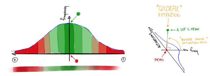\n\n> The idea of the colorful dimension is to express with colors the mean and standard deviation of activations for each batch during training. Vertical axis represents a group (bin) of activation values. Each column in the horizontal axis is a batch. The colours represent how many activations for that batch have a value in that bin.\n\nRef: https://forums.fast.ai/t/the-colorful-dimension/42908","metadata":{}},{"cell_type":"code","source":"def plot_layer_stats(self, idx):\n plt,axs = subplots(1, 3, figsize=(15,3))\n plt.subplots_adjust(wspace=0.5)\n for o,ax,title in zip(self.layer_stats(idx),axs,('mean','std','% near zero')):\n ax.plot(o)\n ax.set_title(f\"{-1*layer}th layer {title}\")","metadata":{"execution":{"iopub.status.busy":"2022-03-29T02:35:09.484157Z","iopub.execute_input":"2022-03-29T02:35:09.4845Z","iopub.status.idle":"2022-03-29T02:35:09.492043Z","shell.execute_reply.started":"2022-03-29T02:35:09.484462Z","shell.execute_reply":"2022-03-29T02:35:09.491268Z"},"trusted":true},"execution_count":null,"outputs":[]},{"cell_type":"code","source":"for layer in range(1,4):\n plot_layer_stats(learn.activation_stats,-1*layer)","metadata":{"execution":{"iopub.status.busy":"2022-03-29T02:35:10.198683Z","iopub.execute_input":"2022-03-29T02:35:10.199526Z","iopub.status.idle":"2022-03-29T02:35:12.240864Z","shell.execute_reply.started":"2022-03-29T02:35:10.199477Z","shell.execute_reply":"2022-03-29T02:35:12.239885Z"},"trusted":true},"execution_count":null,"outputs":[]},{"cell_type":"code","source":"def color_dim(self, idx):\n with plt.rc_context({\"figure.figsize\": (10,40), \"figure.dpi\": (600)}):\n res = self.hist(idx)\n fig = plt.figure()\n ax = fig.add_subplot(111)\n ax.imshow(res, origin='lower')\n ax.set_title(f\"{idx}th activation histogram\")\n ax.axis('off')","metadata":{"execution":{"iopub.status.busy":"2022-03-29T02:35:12.242295Z","iopub.execute_input":"2022-03-29T02:35:12.24314Z","iopub.status.idle":"2022-03-29T02:35:12.249332Z","shell.execute_reply.started":"2022-03-29T02:35:12.243096Z","shell.execute_reply":"2022-03-29T02:35:12.248591Z"},"trusted":true},"execution_count":null,"outputs":[]},{"cell_type":"code","source":"matplotlib.rcParams['image.cmap'] = 'rainbow_r'\nfor layer in range(1,4):\n color_dim(learn.activation_stats,-1*layer)","metadata":{"execution":{"iopub.status.busy":"2022-03-29T02:35:12.250413Z","iopub.execute_input":"2022-03-29T02:35:12.251081Z","iopub.status.idle":"2022-03-29T02:35:16.04558Z","shell.execute_reply.started":"2022-03-29T02:35:12.25103Z","shell.execute_reply":"2022-03-29T02:35:16.044611Z"},"trusted":true},"execution_count":null,"outputs":[]},{"cell_type":"markdown","source":"----------------------------------------------\n# Checking Results","metadata":{}},{"cell_type":"code","source":"plt.rcParams[\"figure.figsize\"] = (8,6)\nlearn.recorder.plot_loss()","metadata":{"execution":{"iopub.status.busy":"2022-03-29T02:35:27.540013Z","iopub.execute_input":"2022-03-29T02:35:27.540325Z","iopub.status.idle":"2022-03-29T02:35:27.75285Z","shell.execute_reply.started":"2022-03-29T02:35:27.540289Z","shell.execute_reply":"2022-03-29T02:35:27.751917Z"},"trusted":true},"execution_count":null,"outputs":[]},{"cell_type":"code","source":"learn.show_results(figsize=(20,20))","metadata":{"execution":{"iopub.status.busy":"2022-03-29T02:35:27.884328Z","iopub.execute_input":"2022-03-29T02:35:27.884618Z","iopub.status.idle":"2022-03-29T02:35:37.944367Z","shell.execute_reply.started":"2022-03-29T02:35:27.884587Z","shell.execute_reply":"2022-03-29T02:35:37.943092Z"},"trusted":true},"execution_count":null,"outputs":[]},{"cell_type":"code","source":"interp = ClassificationInterpretation.from_learner(learn)\ninterp.plot_confusion_matrix(figsize=(15,15),dpi=480)","metadata":{"execution":{"iopub.status.busy":"2022-03-29T02:50:31.556366Z","iopub.execute_input":"2022-03-29T02:50:31.556778Z","iopub.status.idle":"2022-03-29T02:53:24.77744Z","shell.execute_reply.started":"2022-03-29T02:50:31.55674Z","shell.execute_reply":"2022-03-29T02:53:24.776448Z"},"trusted":true},"execution_count":null,"outputs":[]},{"cell_type":"code","source":"interp.most_confused(min_val=5)","metadata":{"execution":{"iopub.status.busy":"2022-03-29T02:45:24.107261Z","iopub.execute_input":"2022-03-29T02:45:24.107758Z","iopub.status.idle":"2022-03-29T02:45:24.115945Z","shell.execute_reply.started":"2022-03-29T02:45:24.107709Z","shell.execute_reply":"2022-03-29T02:45:24.114976Z"},"trusted":true},"execution_count":null,"outputs":[]},{"cell_type":"markdown","source":"-----------------------------\n# Interpreting\n\nWe want to know where we are looking in our model and which points we have decided are important.\nThis allows us to check whether the learning has gone well and whether there is more work to be done to further improve performance.","metadata":{}},{"cell_type":"code","source":"class CaptumInterpretation():\n \"Captum Interpretation for Resnet\"\n def __init__(self,learn,cmap_name='viridis',colors=None,N=256,methods=('original_image','heat_map'),\n signs=(\"all\", \"positive\"),outlier_perc=1):\n if colors is None: colors = [(0, '#ffffff'),(0.25, '#000000'),(1, '#000000')]\n store_attr()\n self.dls,self.model = learn.dls,self.learn.model\n self.supported_metrics=['IG','NT','Occl']\n\n def get_baseline_img(self, img_tensor,baseline_type):\n baseline_img=None\n if baseline_type=='zeros': baseline_img= img_tensor*0\n if baseline_type=='uniform': baseline_img= torch.rand(img_tensor.shape)\n if baseline_type=='gauss':\n baseline_img= (torch.rand(img_tensor.shape).to(self.dls.device)+img_tensor)/2\n return baseline_img.to(self.dls.device)\n\n def visualize(self,inp,metric='IG',n_steps=1000,baseline_type='zeros',nt_type='smoothgrad', strides=(3,4,4), sliding_window_shapes=(3,15,15)):\n if metric not in self.supported_metrics:\n raise Exception(f\"Metric {metric} is not supported. Currently {self.supported_metrics} are only supported\")\n print(inp)\n tls = L([TfmdLists(inp, t) for t in L(ifnone(self.dls.tfms,[None]))])\n inp_data=list(zip(*(tls[0],tls[1])))[0]\n enc_data,dec_data=self._get_enc_dec_data(inp_data)\n attributions=self._get_attributions(enc_data,metric,n_steps,nt_type,baseline_type,strides,sliding_window_shapes)\n self._viz(attributions,dec_data,metric)\n\n def _viz(self,attributions,dec_data,metric):\n default_cmap = LinearSegmentedColormap.from_list(self.cmap_name,self.colors, N=self.N)\n _ = viz.visualize_image_attr_multiple(np.transpose(attributions.squeeze().cpu().detach().numpy(), (1,2,0)),\n np.transpose(dec_data[0].numpy(), (1,2,0)),\n methods=self.methods,\n cmap=default_cmap,\n show_colorbar=True,\n signs=self.signs,\n outlier_perc=self.outlier_perc, titles=[f'Original Image - ({dec_data[1]})', metric])\n\n\n\n def _get_enc_dec_data(self,inp_data):\n dec_data=self.dls.after_item(inp_data)\n enc_data=self.dls.after_batch(to_device(self.dls.before_batch(dec_data),self.dls.device))\n return(enc_data,dec_data)\n\n def _get_attributions(self,enc_data,metric,n_steps,nt_type,baseline_type,strides,sliding_window_shapes):\n # Get Baseline\n baseline=self.get_baseline_img(enc_data[0],baseline_type)\n supported_metrics ={}\n if metric == 'IG':\n self._int_grads = self._int_grads if hasattr(self,'_int_grads') else IntegratedGradients(self.model)\n return self._int_grads.attribute(enc_data[0],baseline, target=enc_data[1], n_steps=200)\n elif metric == 'NT':\n self._int_grads = self._int_grads if hasattr(self,'_int_grads') else IntegratedGradients(self.model)\n self._noise_tunnel= self._noise_tunnel if hasattr(self,'_noise_tunnel') else NoiseTunnel(self._int_grads)\n return self._noise_tunnel.attribute(enc_data[0].to(self.dls.device), n_samples=1, nt_type=nt_type, target=enc_data[1])\n elif metric == 'Occl':\n self._occlusion = self._occlusion if hasattr(self,'_occlusion') else Occlusion(self.model)\n return self._occlusion.attribute(enc_data[0].to(self.dls.device),\n strides = strides,\n target=enc_data[1],\n sliding_window_shapes=sliding_window_shapes,\n baselines=baseline)","metadata":{"execution":{"iopub.status.busy":"2022-03-29T02:45:24.117651Z","iopub.execute_input":"2022-03-29T02:45:24.117941Z","iopub.status.idle":"2022-03-29T02:45:24.14499Z","shell.execute_reply.started":"2022-03-29T02:45:24.117909Z","shell.execute_reply":"2022-03-29T02:45:24.143963Z"},"trusted":true},"execution_count":null,"outputs":[]},{"cell_type":"code","source":"path = '../input/herbarium-2022-fgvc9/train_images/002'\nfnames = get_image_files(path)\nsplits = RandomSplitter(valid_pct=0.2)\ndls = DataBlock(blocks = (ImageBlock, CategoryBlock),\n get_items = get_image_files,\n get_y = parent_label,\n splitter = splits,\n item_tfms=item_tfms).dataloaders(path,bs=16)","metadata":{"execution":{"iopub.status.busy":"2022-03-29T02:35:02.724569Z","iopub.status.idle":"2022-03-29T02:35:02.725386Z","shell.execute_reply.started":"2022-03-29T02:35:02.725085Z","shell.execute_reply":"2022-03-29T02:35:02.725115Z"},"trusted":true},"execution_count":null,"outputs":[]},{"cell_type":"code","source":"learn = cnn_learner(dls, \n xresnet18, \n metrics=[accuracy, top_k_accuracy],\n cbs = [EarlyStoppingCallback(monitor='accuracy', min_delta=0.1, patience=5),ActivationStats(with_hist=True)])","metadata":{"execution":{"iopub.status.busy":"2022-03-29T02:35:02.726488Z","iopub.status.idle":"2022-03-29T02:35:02.726827Z","shell.execute_reply.started":"2022-03-29T02:35:02.726645Z","shell.execute_reply":"2022-03-29T02:35:02.726662Z"},"trusted":true},"execution_count":null,"outputs":[]},{"cell_type":"code","source":"captum=CaptumInterpretation(learn,colors=['green','red','yellow'])\nidx=randint(0,len(fnames))\ncaptum.visualize(fnames[idx])","metadata":{"execution":{"iopub.status.busy":"2022-03-29T02:35:02.728061Z","iopub.status.idle":"2022-03-29T02:35:02.728372Z","shell.execute_reply.started":"2022-03-29T02:35:02.728204Z","shell.execute_reply":"2022-03-29T02:35:02.728221Z"},"trusted":true},"execution_count":null,"outputs":[]},{"cell_type":"code","source":"idx=randint(0,len(fnames))\ncaptum.visualize(fnames[idx],metric='IG',baseline_type='uniform')","metadata":{"execution":{"iopub.status.busy":"2022-03-29T02:35:02.731005Z","iopub.status.idle":"2022-03-29T02:35:02.731614Z","shell.execute_reply.started":"2022-03-29T02:35:02.731432Z","shell.execute_reply":"2022-03-29T02:35:02.731452Z"},"trusted":true},"execution_count":null,"outputs":[]},{"cell_type":"markdown","source":"
","metadata":{}},{"cell_type":"code","source":"","metadata":{},"execution_count":null,"outputs":[]}]}