{"metadata":{"kernelspec":{"language":"python","display_name":"Python 3","name":"python3"},"language_info":{"pygments_lexer":"ipython3","nbconvert_exporter":"python","version":"3.6.4","file_extension":".py","codemirror_mode":{"name":"ipython","version":3},"name":"python","mimetype":"text/x-python"}},"nbformat_minor":4,"nbformat":4,"cells":[{"cell_type":"code","source":"from pathlib import Path\nimport warnings\nwarnings.filterwarnings('ignore')\n\ndata_path = Path(\"../input/google-smartphone-decimeter-challenge\")","metadata":{"execution":{"iopub.status.busy":"2021-09-13T07:31:52.833692Z","iopub.execute_input":"2021-09-13T07:31:52.834247Z","iopub.status.idle":"2021-09-13T07:31:52.846999Z","shell.execute_reply.started":"2021-09-13T07:31:52.834136Z","shell.execute_reply":"2021-09-13T07:31:52.845505Z"},"trusted":true},"execution_count":null,"outputs":[]},{"cell_type":"markdown","source":"# Problem Definition\n## Goal\n\nThis competition, hosted by the Android GPS team, was presented at the ION GNSS+ 2021 Conference. They seek to advance research in smartphone GNSS positioning accuracy and help people better navigate the world around them.\n\nGlobal Navigation Satellite System (GNSS) provides raw signals, which the GPS chipset uses to compute a position. Current mobile phones only offer 3-5 meters of positioning accuracy. While useful in many cases, it can create a “jumpy” experience. For many use cases the results are not fine nor stable enough to be reliable.\n\nThe objective of the competition is that different teams acroos the world could use data collected from the host team’s own Android phones to compute location down to decimeter or even centimeter resolution, if possible. **We'll have access to precise ground truth, raw GPS measurements, and assistance data from nearby GPS stations, in order to train and test your submissions.**\n\nOur submission file is like this.","metadata":{}},{"cell_type":"code","source":"import pandas as pd\n\nsub = pd.read_csv(data_path / \"sample_submission.csv\")\nsub.head()","metadata":{"execution":{"iopub.status.busy":"2021-09-13T07:31:52.869555Z","iopub.execute_input":"2021-09-13T07:31:52.869923Z","iopub.status.idle":"2021-09-13T07:31:53.019891Z","shell.execute_reply.started":"2021-09-13T07:31:52.869894Z","shell.execute_reply":"2021-09-13T07:31:53.018472Z"},"trusted":true},"execution_count":null,"outputs":[]},{"cell_type":"markdown","source":"**latDeg** and **lngDeg** are our target.\n\nWe can use GNSS tracking data and variety of sensor data to improve our solution.\n\n## About dataset \n\nGoogle releases 60+ datasets collected from phones in the Android GPS team, together with corrections from SwiftNavigation Inc. and Verizon Inc. These datasets were collected on highways in the US San Francisco Bay Area in the summer of 2020. We can see the video for dataset.\n\nWe are given data from actual runs with android devices installed in cars, see following.\n\n![](https://raw.githubusercontent.com/tasotasoso/kaggle_media/main/Android_smartphones_high_accuracy_GNSS_datasets/fig3_fig4.JPG)\n\n<font size=\"1\">The figures come from <I>Fu, Guoyu (Michael), Khider, Mohammed, van Diggelen, Frank, \"Android Raw GNSS Measurement Datasets for Precise Positioning,\" Proceedings of the 33rd International Technical Meeting of the Satellite Division of The Institute of Navigation (ION GNSS+ 2020), September 2020, pp. 1925-1937.\n[https://doi.org/10.33012/2020.17628](https://www.ion.org/publications/abstract.cfm?articleID=17628)</I></font>\n\nWe can see more detail of data collection process at [Android smartphones high accuracy GNSS datasets](https://www.kaggle.com/google/android-smartphones-high-accuracy-datasets).","metadata":{}},{"cell_type":"markdown","source":"Data collection trials are separated as collectionName and under each collectionName, the data of the device is stored. In addition, the data collected from each device, groundtruth, and supplemental data are stored under it. The supplemental data contains the raw data that was measured.","metadata":{}},{"cell_type":"markdown","source":"# Basic Data Exploration\n\nThe first step in any machine learning project is familiarize yourself with the data.  You'll use the Pandas library for this.  Pandas is the primary tool data scientists use for exploring and manipulating data. Most people abbreviate pandas in their code as `pd`.  We do this with the command","metadata":{}},{"cell_type":"code","source":"import pandas as pd","metadata":{"execution":{"iopub.status.busy":"2021-09-13T07:31:53.022105Z","iopub.execute_input":"2021-09-13T07:31:53.022504Z","iopub.status.idle":"2021-09-13T07:31:53.028293Z","shell.execute_reply.started":"2021-09-13T07:31:53.022468Z","shell.execute_reply":"2021-09-13T07:31:53.02645Z"},"trusted":true},"execution_count":null,"outputs":[]},{"cell_type":"markdown","source":"## Reading data files\n\n### CSV data files\n\nBeing able to create a DataFrame or Series by hand is handy. But, most of the time, we won't actually be creating our own data by hand. Instead, we'll be working with data that already exists.\n\nData can be stored in any of a number of different forms and formats. By far the most basic of these is the humble CSV file. When you open a CSV file you get something that looks like this:\n\n```\nValue A,Value B,Value C,\n30,21,9,\n35,34,1,\n41,11,11\n```\n\nSo a CSV file is a table of values separated by commas. Hence the name: \"Comma-Separated Values\", or CSV.\n\nLet's now set aside our toy datasets and see what a real dataset looks like when we read it into a DataFrame. We'll use the `pd.read_csv()` function to read the data into a DataFrame. The input data is at the file path **`../input/google-smartphone-decimeter-challenge`**. We will use [train/test]/[drive_id]/[phone_name]/[phone_name]_derived.csv as organized data. And also we can use ground_truth.csv as reference.","metadata":{}},{"cell_type":"code","source":"# read the data and store data in DataFrame\nsample_trail_derived = pd.read_csv(data_path / \"train/2020-05-14-US-MTV-1/Pixel4/Pixel4_derived.csv\")\nsample_trail_truth = pd.read_csv(data_path / \"train/2020-05-14-US-MTV-1/Pixel4/ground_truth.csv\")","metadata":{"execution":{"iopub.status.busy":"2021-09-13T07:31:53.031866Z","iopub.execute_input":"2021-09-13T07:31:53.032777Z","iopub.status.idle":"2021-09-13T07:31:53.402871Z","shell.execute_reply.started":"2021-09-13T07:31:53.032711Z","shell.execute_reply":"2021-09-13T07:31:53.401921Z"},"trusted":true},"execution_count":null,"outputs":[]},{"cell_type":"markdown","source":"We can use the `shape` attribute to check how large the resulting DataFrame is:","metadata":{}},{"cell_type":"code","source":"sample_trail_derived.shape","metadata":{"execution":{"iopub.status.busy":"2021-09-13T07:31:53.404428Z","iopub.execute_input":"2021-09-13T07:31:53.404927Z","iopub.status.idle":"2021-09-13T07:31:53.411607Z","shell.execute_reply.started":"2021-09-13T07:31:53.40489Z","shell.execute_reply":"2021-09-13T07:31:53.410317Z"},"trusted":true},"execution_count":null,"outputs":[]},{"cell_type":"markdown","source":"So our new DataFrame has 55.218 records split across 20 different columns. That's around 1.1 million entries!\n\nWe can examine the contents of the resultant DataFrame using the `head()` command, which grabs the first five rows:","metadata":{}},{"cell_type":"code","source":"sample_trail_derived.head()","metadata":{"execution":{"iopub.status.busy":"2021-09-13T07:31:53.413054Z","iopub.execute_input":"2021-09-13T07:31:53.413383Z","iopub.status.idle":"2021-09-13T07:31:53.455119Z","shell.execute_reply.started":"2021-09-13T07:31:53.413352Z","shell.execute_reply":"2021-09-13T07:31:53.453542Z"},"trusted":true},"execution_count":null,"outputs":[]},{"cell_type":"markdown","source":"We can also have a look at the first rows of the ground truth data frame","metadata":{}},{"cell_type":"code","source":"sample_trail_truth.head()","metadata":{"execution":{"iopub.status.busy":"2021-09-13T07:31:53.457781Z","iopub.execute_input":"2021-09-13T07:31:53.458369Z","iopub.status.idle":"2021-09-13T07:31:53.486734Z","shell.execute_reply.started":"2021-09-13T07:31:53.458307Z","shell.execute_reply":"2021-09-13T07:31:53.485454Z"},"trusted":true},"execution_count":null,"outputs":[]},{"cell_type":"markdown","source":"### Read complex data files (GNSS Log)\n\nThe phone's logs has been generated by the [GnssLogger App](https://play.google.com/store/apps/details?id=com.google.android.apps.location.gps.gnsslogger&hl=en_US&gl=US). Each gnss file contains several sub-datasets:\n* **Raw** - The raw GNSS measurements of one GNSS signal (each satellite may have 1-2 signals for L5-enabled smartphones), collected from the Android API [GnssMeasurement](https://developer.android.com/reference/android/location/GnssMeasurement).\n* **Status** - The status of a GNSS signal, as collected from the Android API [GnssStatus](https://developer.android.com/reference/android/location/GnssStatus.Callback).\n* **UncalAccel** - Readings from the uncalibrated accelerometer, as collected from the Android API [Sensor#TYPE_ACCELEROMETER_UNCALIBRATED](https://developer.android.com/reference/android/hardware/Sensor#TYPE_ACCELEROMETER_UNCALIBRATED).\n* **UncalGyro** - Readings from the uncalibrated gyroscope, as collected from the Android API [Sensor#TYPE_GYROSCOPE_UNCALIBRATED](https://developer.android.com/reference/android/hardware/Sensor#TYPE_GYROSCOPE_UNCALIBRATED).\n* **UncalMag** - Readings from the uncalibrated magnetometer as collected from the Android API [Sensor#STRING_TYPE_MAGNETIC_FIELD_UNCALIBRATED](https://developer.android.com/reference/android/hardware/Sensor#STRING_TYPE_MAGNETIC_FIELD_UNCALIBRATED).\n* **OrientationDeg** - Each row represents an estimated device orientation, collected from Android API [SensorManager#getOrientation](https://developer.android.com/reference/android/hardware/SensorManager#getOrientation%28float%5B%5D,%20float%5B%5D%29). This message is only available in logs collected since March 2021.","metadata":{}},{"cell_type":"code","source":"# Adapted from https://www.kaggle.com/sohier/loading-gnss-logs\ndef gnss_log_to_dataframes(path):\n    print(f'Loading {path}', flush=True)\n    gnss_section_names = {'Raw','UncalAccel', 'UncalGyro', 'UncalMag', 'Fix', 'Status', 'OrientationDeg'}\n    with open(path) as f_open:\n        datalines = f_open.readlines()\n\n    datas = {k: [] for k in gnss_section_names}\n    gnss_map = {k: [] for k in gnss_section_names}\n    for dataline in datalines:\n        is_header = dataline.startswith('#')\n        dataline = dataline.strip('#').strip().split(',')\n        # skip over notes, version numbers, etc\n        if is_header and dataline[0] in gnss_section_names:\n            gnss_map[dataline[0]] = dataline[1:]\n        elif not is_header:\n            datas[dataline[0]].append(dataline[1:])\n\n    results = dict()\n    for k, v in datas.items():\n        results[k] = pd.DataFrame(v, columns=gnss_map[k])\n    # pandas doesn't properly infer types from these lists by default\n    for k, df in results.items():\n        for col in df.columns:\n            if col == 'CodeType':\n                continue\n            results[k][col] = pd.to_numeric(results[k][col])\n\n    return results","metadata":{"execution":{"iopub.status.busy":"2021-09-13T07:31:53.488789Z","iopub.execute_input":"2021-09-13T07:31:53.489281Z","iopub.status.idle":"2021-09-13T07:31:53.501709Z","shell.execute_reply.started":"2021-09-13T07:31:53.489228Z","shell.execute_reply":"2021-09-13T07:31:53.50007Z"},"trusted":true},"execution_count":null,"outputs":[]},{"cell_type":"code","source":"sample_trail_gnss_log = gnss_log_to_dataframes(data_path / \"train/2020-05-14-US-MTV-1/Pixel4/Pixel4_GnssLog.txt\")\nsample_trail_gnss_log.keys()","metadata":{"execution":{"iopub.status.busy":"2021-09-13T07:31:53.503542Z","iopub.execute_input":"2021-09-13T07:31:53.503928Z","iopub.status.idle":"2021-09-13T07:32:19.898418Z","shell.execute_reply.started":"2021-09-13T07:31:53.503885Z","shell.execute_reply":"2021-09-13T07:32:19.897277Z"},"trusted":true},"execution_count":null,"outputs":[]},{"cell_type":"markdown","source":"We´ve got a dictionary with one key per each sub-dataset. We can have a look at the first rows of the *Raw* dataset.","metadata":{}},{"cell_type":"code","source":"raw_gnss = sample_trail_gnss_log['Raw']\nraw_gnss.head()","metadata":{"execution":{"iopub.status.busy":"2021-09-13T07:32:19.901376Z","iopub.execute_input":"2021-09-13T07:32:19.901785Z","iopub.status.idle":"2021-09-13T07:32:19.939167Z","shell.execute_reply.started":"2021-09-13T07:32:19.901747Z","shell.execute_reply":"2021-09-13T07:32:19.936837Z"},"trusted":true},"execution_count":null,"outputs":[]},{"cell_type":"markdown","source":"## Indexing, Selecting & Assigning\n\nSelecting specific values of a pandas DataFrame or Series to work on is an implicit step in almost any data operation we'll run, so one of the first things you need to learn in working with data in Python is how to go about selecting the data points relevant to us quickly and effectively.\n\nHence to access the `constellationType` property of `derived` data we can use:","metadata":{}},{"cell_type":"code","source":"sample_trail_derived.constellationType # Or sample_trail_derived['constellationType']","metadata":{"execution":{"iopub.status.busy":"2021-09-13T07:32:19.941363Z","iopub.execute_input":"2021-09-13T07:32:19.941749Z","iopub.status.idle":"2021-09-13T07:32:19.951116Z","shell.execute_reply.started":"2021-09-13T07:32:19.941714Z","shell.execute_reply":"2021-09-13T07:32:19.949933Z"},"trusted":true},"execution_count":null,"outputs":[]},{"cell_type":"markdown","source":"To select the first row of data in a DataFrame, we may use the following:","metadata":{}},{"cell_type":"code","source":"sample_trail_derived.iloc[0]","metadata":{"execution":{"iopub.status.busy":"2021-09-13T07:32:19.952842Z","iopub.execute_input":"2021-09-13T07:32:19.953279Z","iopub.status.idle":"2021-09-13T07:32:19.967851Z","shell.execute_reply.started":"2021-09-13T07:32:19.95324Z","shell.execute_reply":"2021-09-13T07:32:19.966726Z"},"trusted":true},"execution_count":null,"outputs":[]},{"cell_type":"markdown","source":"## Conditional selection\n\nSo far we've been indexing various strides of data, using structural properties of the DataFrame itself. To do *interesting* things with the data, however, we often need to ask questions based on conditions. \n\nFor example, suppose that we're interested specifically in Galileo E1 signal types.\n\nWe can start by checking if each entry is a Galileo E1 signal types:","metadata":{}},{"cell_type":"code","source":"sample_trail_derived.signalType == 'GAL_E1'","metadata":{"execution":{"iopub.status.busy":"2021-09-13T07:32:19.969588Z","iopub.execute_input":"2021-09-13T07:32:19.970188Z","iopub.status.idle":"2021-09-13T07:32:19.995373Z","shell.execute_reply.started":"2021-09-13T07:32:19.970143Z","shell.execute_reply":"2021-09-13T07:32:19.994249Z"},"trusted":true},"execution_count":null,"outputs":[]},{"cell_type":"markdown","source":"This operation produced a Series of True/False booleans based on the signal type of each record. This result can then be used inside of loc to select the relevant data:","metadata":{}},{"cell_type":"code","source":"sample_trail_derived.loc[sample_trail_derived.signalType == 'GAL_E1']","metadata":{"execution":{"iopub.status.busy":"2021-09-13T07:32:19.997166Z","iopub.execute_input":"2021-09-13T07:32:19.997542Z","iopub.status.idle":"2021-09-13T07:32:20.06012Z","shell.execute_reply.started":"2021-09-13T07:32:19.997506Z","shell.execute_reply":"2021-09-13T07:32:20.058859Z"},"trusted":true},"execution_count":null,"outputs":[]},{"cell_type":"markdown","source":"This DataFrame has ~11,000 rows. The original had ~55,000. That means that around 20% of the entries have signal type Galileo E1.\n\nIf we also wanted to select entries from satellite id 13 or 15, we can use the ampersand (`&`) to bring the two questions together:","metadata":{}},{"cell_type":"code","source":"sample_trail_derived.loc[(sample_trail_derived.signalType == 'GAL_E1') & (sample_trail_derived.svid.isin([13, 15]))]","metadata":{"execution":{"iopub.status.busy":"2021-09-13T07:32:20.061938Z","iopub.execute_input":"2021-09-13T07:32:20.062439Z","iopub.status.idle":"2021-09-13T07:32:20.120646Z","shell.execute_reply.started":"2021-09-13T07:32:20.062368Z","shell.execute_reply":"2021-09-13T07:32:20.119373Z"},"trusted":true},"execution_count":null,"outputs":[]},{"cell_type":"markdown","source":"Suppose we want to filter for any Galileo E1 or GPS L5 sygnal type. For this we use a pipe (`|`):","metadata":{}},{"cell_type":"code","source":"sample_trail_derived.loc[(sample_trail_derived.signalType == 'GAL_E1') | (sample_trail_derived.signalType == 'GPS_L5')]","metadata":{"execution":{"iopub.status.busy":"2021-09-13T07:32:20.122173Z","iopub.execute_input":"2021-09-13T07:32:20.122555Z","iopub.status.idle":"2021-09-13T07:32:20.190748Z","shell.execute_reply.started":"2021-09-13T07:32:20.122509Z","shell.execute_reply":"2021-09-13T07:32:20.189611Z"},"trusted":true},"execution_count":null,"outputs":[]},{"cell_type":"markdown","source":"## Summary Functions\n\nPandas provides many simple \"summary functions\" which restructure the data in some useful way. For example, let´s consider the describe() method to review the carrier-to-noise density in dB-Hz.:","metadata":{}},{"cell_type":"code","source":"raw_gnss.Cn0DbHz.describe()","metadata":{"execution":{"iopub.status.busy":"2021-09-13T07:32:20.192399Z","iopub.execute_input":"2021-09-13T07:32:20.19279Z","iopub.status.idle":"2021-09-13T07:32:20.208685Z","shell.execute_reply.started":"2021-09-13T07:32:20.192753Z","shell.execute_reply":"2021-09-13T07:32:20.207762Z"},"trusted":true},"execution_count":null,"outputs":[]},{"cell_type":"markdown","source":"This method generates a high-level summary of the attributes of the given column. It is type-aware, meaning that its output changes based on the data type of the input. The output above only makes sense for numerical data; for string data here's what we get:","metadata":{}},{"cell_type":"code","source":"sample_trail_derived.signalType.describe()","metadata":{"execution":{"iopub.status.busy":"2021-09-13T07:32:20.209992Z","iopub.execute_input":"2021-09-13T07:32:20.210301Z","iopub.status.idle":"2021-09-13T07:32:20.255024Z","shell.execute_reply.started":"2021-09-13T07:32:20.210272Z","shell.execute_reply":"2021-09-13T07:32:20.253873Z"},"trusted":true},"execution_count":null,"outputs":[]},{"cell_type":"markdown","source":"If you want to get some particular simple summary statistic about a column in a DataFrame or a Series, there is usually a helpful pandas function that makes it happen. \n\nFor example, to see the mean of the points allotted (e.g. how well an averagely rated wine does), we can use the `mean()` function:","metadata":{}},{"cell_type":"code","source":"raw_gnss.Cn0DbHz.mean()","metadata":{"execution":{"iopub.status.busy":"2021-09-13T07:32:20.256715Z","iopub.execute_input":"2021-09-13T07:32:20.257163Z","iopub.status.idle":"2021-09-13T07:32:20.267567Z","shell.execute_reply.started":"2021-09-13T07:32:20.257116Z","shell.execute_reply":"2021-09-13T07:32:20.266503Z"},"trusted":true},"execution_count":null,"outputs":[]},{"cell_type":"markdown","source":"To see a list of unique values we can use the `unique()` function:","metadata":{}},{"cell_type":"code","source":"sample_trail_derived.signalType.unique()","metadata":{"execution":{"iopub.status.busy":"2021-09-13T07:32:20.269281Z","iopub.execute_input":"2021-09-13T07:32:20.269957Z","iopub.status.idle":"2021-09-13T07:32:20.284303Z","shell.execute_reply.started":"2021-09-13T07:32:20.26991Z","shell.execute_reply":"2021-09-13T07:32:20.283315Z"},"trusted":true},"execution_count":null,"outputs":[]},{"cell_type":"markdown","source":"To see a list of unique values _and_ how often they occur in the dataset, we can use the `value_counts()` method:","metadata":{}},{"cell_type":"code","source":"sample_trail_derived.signalType.value_counts()","metadata":{"execution":{"iopub.status.busy":"2021-09-13T07:32:20.285996Z","iopub.execute_input":"2021-09-13T07:32:20.286501Z","iopub.status.idle":"2021-09-13T07:32:20.310249Z","shell.execute_reply.started":"2021-09-13T07:32:20.286454Z","shell.execute_reply":"2021-09-13T07:32:20.309337Z"},"trusted":true},"execution_count":null,"outputs":[]},{"cell_type":"markdown","source":"## Data Types and Missing Values\n\nThe data type for a column in a DataFrame or a Series is known as the **dtype**.\n\nWe can use the `dtype` property to grab the type of a specific column.  For instance, we can get the dtype of the `Cn0DbHz` column in the `derived` DataFrame:","metadata":{}},{"cell_type":"code","source":"raw_gnss.Cn0DbHz.dtype","metadata":{"execution":{"iopub.status.busy":"2021-09-13T07:32:20.311725Z","iopub.execute_input":"2021-09-13T07:32:20.312231Z","iopub.status.idle":"2021-09-13T07:32:20.319365Z","shell.execute_reply.started":"2021-09-13T07:32:20.312182Z","shell.execute_reply":"2021-09-13T07:32:20.317899Z"},"trusted":true},"execution_count":null,"outputs":[]},{"cell_type":"markdown","source":"Alternatively, the `info` method returns the `dtype` of _every_ column in the DataFrame and the number of non-empty values:","metadata":{}},{"cell_type":"code","source":"sample_trail_derived.info()","metadata":{"execution":{"iopub.status.busy":"2021-09-13T07:32:20.321202Z","iopub.execute_input":"2021-09-13T07:32:20.321915Z","iopub.status.idle":"2021-09-13T07:32:20.364021Z","shell.execute_reply.started":"2021-09-13T07:32:20.321861Z","shell.execute_reply":"2021-09-13T07:32:20.363147Z"},"trusted":true},"execution_count":null,"outputs":[]},{"cell_type":"markdown","source":"## Data Visualization\n\n### Visualize a track with Plotly\n","metadata":{}},{"cell_type":"code","source":"import plotly.express as px\n\n# from https://www.kaggle.com/nayuts/let-s-visualize-dataset-to-understand\ndef visualize_trafic(df, center, zoom=9):\n    fig = px.scatter_mapbox(df,\n                            \n                            # Here, plotly gets, (x,y) coordinates\n                            lat=\"latDeg\",\n                            lon=\"lngDeg\",\n                            \n                            #Here, plotly detects color of series\n                            color=\"phoneName\",\n                            labels=\"phoneName\",\n                            \n                            zoom=zoom,\n                            center=center,\n                            height=600,\n                            width=800)\n    fig.update_layout(mapbox_style='stamen-terrain')\n    fig.update_layout(margin={\"r\": 0, \"t\": 0, \"l\": 0, \"b\": 0})\n    fig.update_layout(title_text=\"GPS trafic\")\n    fig.show()","metadata":{"execution":{"iopub.status.busy":"2021-09-13T07:32:20.36515Z","iopub.execute_input":"2021-09-13T07:32:20.365588Z","iopub.status.idle":"2021-09-13T07:32:21.681782Z","shell.execute_reply.started":"2021-09-13T07:32:20.365555Z","shell.execute_reply":"2021-09-13T07:32:21.68055Z"},"trusted":true},"execution_count":null,"outputs":[]},{"cell_type":"code","source":"center = {\"lat\":37.423576, \"lon\":-122.094132}\nvisualize_trafic(sample_trail_truth, center)","metadata":{"execution":{"iopub.status.busy":"2021-09-13T07:32:21.685874Z","iopub.execute_input":"2021-09-13T07:32:21.686262Z","iopub.status.idle":"2021-09-13T07:32:22.513427Z","shell.execute_reply.started":"2021-09-13T07:32:21.686227Z","shell.execute_reply":"2021-09-13T07:32:22.512623Z"},"trusted":true},"execution_count":null,"outputs":[]},{"cell_type":"markdown","source":"Let´s now plot data which have same collectionName to see if they have the same ground truth.","metadata":{}},{"cell_type":"code","source":"sample_trail_2_truth = pd.read_csv(data_path / \"train/2020-05-14-US-MTV-1/Pixel4XLModded/ground_truth.csv\")\n\n# Since plotly looks at the phoneName of the dataframe,\n# you can visualize multiple series of data by simply concatting dataframes.\nsample_trail_truth_combined = pd.concat([sample_trail_truth, sample_trail_2_truth])\n\ncenter = {\"lat\":37.423576, \"lon\":-122.094132}\nvisualize_trafic(sample_trail_truth_combined, center)","metadata":{"execution":{"iopub.status.busy":"2021-09-13T07:32:22.514592Z","iopub.execute_input":"2021-09-13T07:32:22.515046Z","iopub.status.idle":"2021-09-13T07:32:22.618235Z","shell.execute_reply.started":"2021-09-13T07:32:22.515013Z","shell.execute_reply":"2021-09-13T07:32:22.617336Z"},"trusted":true},"execution_count":null,"outputs":[]},{"cell_type":"markdown","source":"### Visualize multiple tracks with GeoPandas\n\nIn the previous step we saw how to use plotly to map data on OpenStreetMap. This time, since there is a certain amount of tracking data in the train data alone, we will see how to use geopandas to get a quick overview as a regular diagram.\n\nFirst, we'll download shape file lof bayarea.","metadata":{}},{"cell_type":"code","source":"import geopandas as gpd\nfrom geopandas import GeoDataFrame\nimport requests\nfrom shapely.geometry import Point, shape\nimport shapely.wkt\n\n#Download geojson file of US San Francisco Bay Area.\nr = requests.get(\"https://data.sfgov.org/api/views/wamw-vt4s/rows.json?accessType=DOWNLOAD\")\nr.raise_for_status()\n\n#get geojson from response\ndata = r.json()\n\n#get polygons that represents San Francisco Bay Area.\nshapes = []\nfor d in data[\"data\"]:\n    shapes.append(shapely.wkt.loads(d[8]))\n    \n#Convert list of porygons to geopandas dataframe.\ngdf_bayarea = pd.DataFrame()\n\n#I'll use only 6 and 7th object.\nfor shp in shapes[5:7]:\n    tmp = pd.DataFrame(shp, columns=[\"geometry\"])\n    gdf_bayarea = pd.concat([gdf_bayarea, tmp])\n    \ngdf_bayarea = GeoDataFrame(gdf_bayarea)","metadata":{"execution":{"iopub.status.busy":"2021-09-13T07:32:22.619678Z","iopub.execute_input":"2021-09-13T07:32:22.620008Z","iopub.status.idle":"2021-09-13T07:32:24.34839Z","shell.execute_reply.started":"2021-09-13T07:32:22.619975Z","shell.execute_reply":"2021-09-13T07:32:24.34691Z"},"trusted":true},"execution_count":null,"outputs":[]},{"cell_type":"markdown","source":"For each collectionNames, read the ground truth files in format that is convenient for visualization. At this time, we have already converted it to geopandas dataframe.","metadata":{}},{"cell_type":"code","source":"import glob\n\ncollectionNames = [item.split(\"/\")[-1] for item in glob.glob(\"../input/google-smartphone-decimeter-challenge/train/*\")]\n\ngdfs = []\nfor collectionName in collectionNames:\n    gdfs_each_collectionName = []\n    csv_paths = glob.glob(f\"../input/google-smartphone-decimeter-challenge/train/{collectionName}/*/ground_truth.csv\")\n    for csv_path in csv_paths:\n        df_gt = pd.read_csv(csv_path)\n        df_gt[\"geometry\"] = [Point(lngDeg, latDeg) for lngDeg, latDeg in zip(df_gt[\"lngDeg\"], df_gt[\"latDeg\"])]\n        gdfs_each_collectionName.append(GeoDataFrame(df_gt))\n    gdfs.append(gdfs_each_collectionName)\n    \ncolors = ['blue', 'green', 'purple', 'orange']","metadata":{"execution":{"iopub.status.busy":"2021-09-13T07:32:24.354746Z","iopub.execute_input":"2021-09-13T07:32:24.355142Z","iopub.status.idle":"2021-09-13T07:32:26.878881Z","shell.execute_reply.started":"2021-09-13T07:32:24.355094Z","shell.execute_reply":"2021-09-13T07:32:26.87779Z"},"trusted":true},"execution_count":null,"outputs":[]},{"cell_type":"markdown","source":"Now, let's visualize tracks. Some of them were too small to be seen when projected on the map, so we put them side by side with the ones that are just routes.","metadata":{}},{"cell_type":"code","source":"import matplotlib.pyplot as plt\n\nfor collectionName, gdfs_each_collectionName in zip(collectionNames, gdfs):\n    fig, axs = plt.subplots(1, 2, figsize=(15, 5))\n    gdf_bayarea.plot(figsize=(10,10), color='none', edgecolor='gray', zorder=3, ax=axs[0])\n    for i, gdf in enumerate(gdfs_each_collectionName):\n        g1 = gdf.plot(color=colors[i], ax=axs[0])\n        g1.set_title(f\"Phone track of {collectionName} with map\")\n        g2 = gdf.plot(color=colors[i], ax=axs[1])\n        g2.set_title(f\"Phone track of {collectionName}\")","metadata":{"execution":{"iopub.status.busy":"2021-09-13T07:32:26.881257Z","iopub.execute_input":"2021-09-13T07:32:26.881716Z","iopub.status.idle":"2021-09-13T07:33:10.287082Z","shell.execute_reply.started":"2021-09-13T07:32:26.881676Z","shell.execute_reply":"2021-09-13T07:33:10.285807Z"},"trusted":true},"execution_count":null,"outputs":[]},{"cell_type":"markdown","source":"There are several tracks that have the same form of data with different collectionName. It is easy to understand the positional relationship by overlapping them. There are two roads extending from the northwest to the southeast, and they seem to run along those roads all the time, or occasionally go off those roads. The tracks wandering around the grid-like paths seem to be collected farther southeast than those paths.","metadata":{}},{"cell_type":"code","source":"fig, ax = plt.subplots(figsize=(15, 5))\n\nfor collectionName, gdfs_each_collectionName in zip(collectionNames, gdfs):   \n    for i, gdf in enumerate(gdfs_each_collectionName):\n        gdf.plot(color=colors[i], ax=ax, markersize=5, alpha=0.5)","metadata":{"execution":{"iopub.status.busy":"2021-09-13T07:33:10.288848Z","iopub.execute_input":"2021-09-13T07:33:10.289179Z","iopub.status.idle":"2021-09-13T07:33:37.833006Z","shell.execute_reply.started":"2021-09-13T07:33:10.289147Z","shell.execute_reply":"2021-09-13T07:33:37.831701Z"},"trusted":true},"execution_count":null,"outputs":[]},{"cell_type":"markdown","source":"In geopandas, it's easy to see where they are in relation to each other, but it's hard to see the details and geographic information, so let's look at them with plotly as well","metadata":{}},{"cell_type":"code","source":"all_tracks = pd.DataFrame()\n\nfor collectionName, gdfs_each_collectionName in zip(collectionNames, gdfs):   \n    for i, gdf in enumerate(gdfs_each_collectionName):\n        all_tracks = pd.concat([all_tracks, gdf])\n        # Tracks they have same collectionName is also same\n        break\n        \nfig = px.scatter_mapbox(all_tracks,\n                            \n                        # Here, plotly gets, (x,y) coordinates\n                        lat=\"latDeg\",\n                        lon=\"lngDeg\",\n                            \n                        #Here, plotly detects color of series\n                        color=\"collectionName\",\n                        labels=\"collectionName\",\n                            \n                        zoom=9,\n                        center={\"lat\":37.423576, \"lon\":-122.094132},\n                        height=600,\n                        width=800)\nfig.update_layout(mapbox_style='stamen-terrain')\nfig.update_layout(margin={\"r\": 0, \"t\": 0, \"l\": 0, \"b\": 0})\nfig.update_layout(title_text=\"GPS trafic\")\nfig.show()","metadata":{"execution":{"iopub.status.busy":"2021-09-13T07:33:37.834955Z","iopub.execute_input":"2021-09-13T07:33:37.835311Z","iopub.status.idle":"2021-09-13T07:33:39.037722Z","shell.execute_reply.started":"2021-09-13T07:33:37.835276Z","shell.execute_reply":"2021-09-13T07:33:39.036026Z"},"trusted":true},"execution_count":null,"outputs":[]},{"cell_type":"markdown","source":"### Visualize Heatmap for Geo-Data with Folium","metadata":{}},{"cell_type":"code","source":"# from https://www.kaggle.com/dannellyz/start-here-simple-folium-heatmap-for-geo-data\nimport folium\nfrom folium import plugins\n\n\ndef simple_folium(df:pd.DataFrame, lat_col:str, lon_col:str):\n    \"\"\"\n    Descrption\n    ----------\n        Returns a simple Folium HeatMap with Markers\n    ----------\n    Parameters\n    ----------\n        df : padnas DataFrame, required\n            The DataFrane with the data to map\n        lat_col : str, required\n            The name of the column with latitude\n        lon_col : str, required\n            The name of the column with longitude\n    \"\"\"\n    #Preprocess\n    #Drop rows that do not have lat/lon\n    df = df[df[lat_col].notnull() & df[lon_col].notnull()]\n\n    # Convert lat/lon to (n, 2) nd-array format for heatmap\n    # Then send to list\n    df_locs = list(df[[lat_col, lon_col]].values)\n\n    #Set up folium map\n    fol_map = folium.Map([df[lat_col].median(), df[lon_col].median()])\n\n    # plot heatmap\n    heat_map = plugins.HeatMap(df_locs)\n    fol_map.add_child(heat_map)\n\n    # plot markers\n    markers = plugins.MarkerCluster(locations = df_locs)\n    fol_map.add_child(markers)\n\n    #Add Layer Control\n    folium.LayerControl().add_to(fol_map)\n\n    return fol_map","metadata":{"execution":{"iopub.status.busy":"2021-09-13T07:33:39.039823Z","iopub.execute_input":"2021-09-13T07:33:39.040527Z","iopub.status.idle":"2021-09-13T07:33:39.496594Z","shell.execute_reply.started":"2021-09-13T07:33:39.040466Z","shell.execute_reply":"2021-09-13T07:33:39.495396Z"},"trusted":true},"execution_count":null,"outputs":[]},{"cell_type":"markdown","source":"First, let's see how estimated locations between the training and test data look like. The ground truth for training data is available per phone in {collectionName}/{phoneName}/ground_truth.csv.","metadata":{}},{"cell_type":"code","source":"train_baseline_locations = pd.read_csv(data_path / 'baseline_locations_train.csv')\nlatlon_trn = train_baseline_locations[['latDeg', 'lngDeg']].round(3)\nlatlon_trn['counts'] = 1\nlatlon_trn = latlon_trn.groupby(['latDeg', 'lngDeg']).sum().reset_index()\nlatlon_trn.head()","metadata":{"execution":{"iopub.status.busy":"2021-09-13T07:33:39.498626Z","iopub.execute_input":"2021-09-13T07:33:39.499128Z","iopub.status.idle":"2021-09-13T07:33:39.766922Z","shell.execute_reply.started":"2021-09-13T07:33:39.499072Z","shell.execute_reply":"2021-09-13T07:33:39.765725Z"},"trusted":true},"execution_count":null,"outputs":[]},{"cell_type":"markdown","source":"Let's see the heatmap for the training data.","metadata":{}},{"cell_type":"code","source":"simple_folium(latlon_trn, 'latDeg', 'lngDeg')","metadata":{"execution":{"iopub.status.busy":"2021-09-13T07:33:39.768446Z","iopub.execute_input":"2021-09-13T07:33:39.768771Z","iopub.status.idle":"2021-09-13T07:33:41.27952Z","shell.execute_reply.started":"2021-09-13T07:33:39.768741Z","shell.execute_reply":"2021-09-13T07:33:41.278024Z"},"trusted":true},"execution_count":null,"outputs":[]},{"cell_type":"markdown","source":"Let's see the heatmap for the test data too","metadata":{}},{"cell_type":"code","source":"test_baseline_locations = pd.read_csv(data_path / 'baseline_locations_test.csv')\nlatlon_tst = test_baseline_locations[['latDeg', 'lngDeg']].round(3)\nlatlon_tst['counts'] = 1\nlatlon_tst = latlon_tst.groupby(['latDeg', 'lngDeg']).sum().reset_index()\n\nsimple_folium(latlon_tst, 'latDeg', 'lngDeg')","metadata":{"execution":{"iopub.status.busy":"2021-09-13T07:33:41.280931Z","iopub.execute_input":"2021-09-13T07:33:41.281429Z","iopub.status.idle":"2021-09-13T07:33:42.982338Z","shell.execute_reply.started":"2021-09-13T07:33:41.281375Z","shell.execute_reply":"2021-09-13T07:33:42.980673Z"},"trusted":true},"execution_count":null,"outputs":[]},{"cell_type":"markdown","source":"## Feature Engineering\n\nThe goal of feature engineering is simply to make our data better suited to the problem at hand. We might perform feature engineering to:\n- improve a model's predictive performance\n- reduce computational or data needs\n- improve interpretability of the results\n\n### A Guiding Principle of Feature Engineering\n\nFor a feature to be useful, it must have a relationship to the target that your model is able to learn. Linear models, for instance, are only able to learn linear relationships. So, when using a linear model, your goal is to transform the features to make their relationship to the target linear.\n\nWhatever relationships our model can't learn, we can provide ourself through transformations. As we develop our feature set, think about what information our model could use to achieve its best performance. \n\n#### Corrected Pseudo Range\n\nLet's calculate a corrected pseudorange (i.e. a closer approximation to the geometric range from the phone to the satellite) as described in the data description:\n```\ncorrectedPrM = rawPrM + satClkBiasM - isrbM - ionoDelayM - tropoDelayM\n```\n\"The baseline locations are computed using correctedPrM and the satellite positions, using a standard Weighted Least Squares (WLS) solver, with the phone's position (x, y, z), clock bias (t), and isrbM for each unique signal type as states for each epoch.\"","metadata":{}},{"cell_type":"code","source":"sample_trail_derived['correctedPrM'] = (sample_trail_derived.rawPrM + sample_trail_derived.satClkBiasM - sample_trail_derived.isrbM - \n                        sample_trail_derived.ionoDelayM - sample_trail_derived.tropoDelayM)\nsample_trail_derived.head()","metadata":{"execution":{"iopub.status.busy":"2021-09-13T07:33:42.984378Z","iopub.execute_input":"2021-09-13T07:33:42.984896Z","iopub.status.idle":"2021-09-13T07:33:43.037452Z","shell.execute_reply.started":"2021-09-13T07:33:42.984844Z","shell.execute_reply":"2021-09-13T07:33:43.03626Z"},"trusted":true},"execution_count":null,"outputs":[]},{"cell_type":"markdown","source":"#### Previous location\n\nWe can add previous latitude and longitude estimates as features.","metadata":{}},{"cell_type":"code","source":"train_baseline_locations.columns","metadata":{"execution":{"iopub.status.busy":"2021-09-13T07:33:43.039256Z","iopub.execute_input":"2021-09-13T07:33:43.039976Z","iopub.status.idle":"2021-09-13T07:33:43.047875Z","shell.execute_reply.started":"2021-09-13T07:33:43.039919Z","shell.execute_reply":"2021-09-13T07:33:43.046631Z"},"trusted":true},"execution_count":null,"outputs":[]},{"cell_type":"code","source":"train_baseline_locations.sort_values(['phone', 'millisSinceGpsEpoch'], inplace=True)\ntrain_baseline_locations[['prev_lat']] = train_baseline_locations['latDeg'].shift().where(train_baseline_locations['phone'].eq(train_baseline_locations['phone'].shift()))\ntrain_baseline_locations[['prev_lon']] = train_baseline_locations['lngDeg'].shift().where(train_baseline_locations['phone'].eq(train_baseline_locations['phone'].shift()))\n\ntest_baseline_locations.sort_values(['phone', 'millisSinceGpsEpoch'], inplace=True)\ntest_baseline_locations[['prev_lat']] = test_baseline_locations['latDeg'].shift().where(test_baseline_locations['phone'].eq(test_baseline_locations['phone'].shift()))\ntest_baseline_locations[['prev_lon']] = test_baseline_locations['lngDeg'].shift().where(test_baseline_locations['phone'].eq(test_baseline_locations['phone'].shift()))\n\ntest_baseline_locations.head()","metadata":{"execution":{"iopub.status.busy":"2021-09-13T07:33:43.05006Z","iopub.execute_input":"2021-09-13T07:33:43.050619Z","iopub.status.idle":"2021-09-13T07:33:43.246929Z","shell.execute_reply.started":"2021-09-13T07:33:43.050572Z","shell.execute_reply":"2021-09-13T07:33:43.245733Z"},"trusted":true},"execution_count":null,"outputs":[]},{"cell_type":"markdown","source":"# Create a Machine Learning Model\n\nIn this example we will apply a Kalman Filter to improve the baseline slightly. \n\n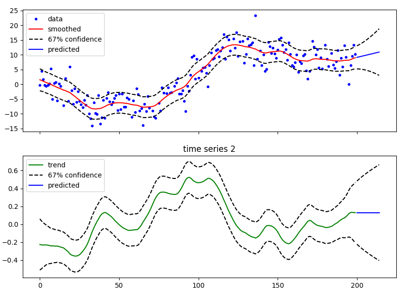![Drag Racing](https://simdkalman.readthedocs.io/en/latest/_images/example.png)\n\nPlease read the documentation if you would like to learn more about this implementation of kf: https://simdkalman.readthedocs.io/en/latest/","metadata":{}},{"cell_type":"code","source":"!pip install simdkalman\n\nfrom pathlib import Path\nimport numpy as np\nimport pandas as pd\nimport simdkalman\nfrom tqdm.notebook import tqdm","metadata":{"_uuid":"8f2839f25d086af736a60e9eeb907d3b93b6e0e5","_cell_guid":"b1076dfc-b9ad-4769-8c92-a6c4dae69d19","execution":{"iopub.status.busy":"2021-09-13T07:33:43.248635Z","iopub.execute_input":"2021-09-13T07:33:43.248983Z","iopub.status.idle":"2021-09-13T07:33:50.547351Z","shell.execute_reply.started":"2021-09-13T07:33:43.248949Z","shell.execute_reply":"2021-09-13T07:33:50.545877Z"},"trusted":true},"execution_count":null,"outputs":[]},{"cell_type":"markdown","source":"## Define Model\n","metadata":{}},{"cell_type":"code","source":"# from https://www.kaggle.com/jpmiller/baseline-from-host-data\nT = 1.0\nstate_transition = np.array([[1, 0, T, 0, 0.5 * T ** 2, 0], [0, 1, 0, T, 0, 0.5 * T ** 2], [0, 0, 1, 0, T, 0],\n                             [0, 0, 0, 1, 0, T], [0, 0, 0, 0, 1, 0], [0, 0, 0, 0, 0, 1]])\nprocess_noise = np.diag([1e-5, 1e-5, 5e-6, 5e-6, 1e-6, 1e-6]) + np.ones((6, 6)) * 1e-9\nobservation_model = np.array([[1, 0, 0, 0, 0, 0], [0, 1, 0, 0, 0, 0]])\nobservation_noise = np.diag([5e-5, 5e-5]) + np.ones((2, 2)) * 1e-9\n\nkf = simdkalman.KalmanFilter(\n        state_transition = state_transition,\n        process_noise = process_noise,\n        observation_model = observation_model,\n        observation_noise = observation_noise)\n\ndef apply_kf_smoothing(df, kf_=kf):\n    unique_paths = df[['collectionName', 'phoneName']].drop_duplicates().to_numpy()\n    for collection, phone in tqdm(unique_paths):\n        cond = np.logical_and(df['collectionName'] == collection, df['phoneName'] == phone)\n        data = df[cond][['latDeg', 'lngDeg']].to_numpy()\n        data = data.reshape(1, len(data), 2)\n        smoothed = kf_.smooth(data)\n        df.loc[cond, 'latDeg'] = smoothed.states.mean[0, :, 0]\n        df.loc[cond, 'lngDeg'] = smoothed.states.mean[0, :, 1]\n    return df","metadata":{"execution":{"iopub.status.busy":"2021-09-13T07:33:50.564476Z","iopub.execute_input":"2021-09-13T07:33:50.565502Z","iopub.status.idle":"2021-09-13T07:33:50.5781Z","shell.execute_reply.started":"2021-09-13T07:33:50.565433Z","shell.execute_reply":"2021-09-13T07:33:50.576638Z"},"trusted":true},"execution_count":null,"outputs":[]},{"cell_type":"markdown","source":"# Model Validation\n\nWe've built a model. But how good is it?\n\nNow we will learn to use model validation to measure the quality of our model. Measuring model quality is the key to iteratively improving your models.\n\n## What is Model Validation\nWe'll want to evaluate almost every model we ever build. In most (though not all) applications, the relevant measure of model quality is predictive accuracy. In other words, will the model's predictions be close to what actually happens.\n\nMany people make a huge mistake when measuring predictive accuracy. They make predictions with their training data and compare those predictions to the target values in the training data. We'll see the problem with this approach and how to solve it in a moment, but let's think about how we'd do this first.\n\nYou'd first need to summarize the model quality into an understandable way. If you compare predicted and actual phone positions, we'll likely find mix of good and bad predictions. Looking through a list of undred of thousands predicted and actual values would be pointless. We need to summarize this into a single metric.\n\nThere are many metrics for summarizing model quality, but we'll start with one called **Mean Absolute Error** (also called **MAE**). Let's break down this metric starting with the last word, error.\n\nThe prediction error for each position is: <br>\n```\nerror = haversine_distance(actual_position, predicted_position)\n```\n\nSo, if a phone is at 50° 03′ 59″ N, 005° 42′ 53″ W and our position prediction is at 50° 03′ 59″ N, 005° 42′ 53.1″ W the error is 1.98m.\n\nWith the MAE metric, we take the absolute value of each error. This converts each error to a positive number. We then take the average of those absolute errors. This is our measure of model quality. In plain English, it can be said as\n\n> On average, our predictions are off by about X.\n\nMAE is not the only measure that can be used to summarize model quality. For example, in the case of the Google Smartphone Decimeter Challenge, submissions are socred on the mean of the **50th and 95th percentile distance errors**.","metadata":{}},{"cell_type":"code","source":"# Simplified haversine distance\ndef haversine_distance(lat1: float, lon1: float, lat2: float, lon2: float):\n    \"\"\"Calculates the great circle distance between two points\n    on the earth. Inputs are array-like and specified in decimal degrees.\n    \"\"\"\n    lat1, lon1, lat2, lon2 = map(np.radians, [lat1, lon1, lat2, lon2])\n    dlat = lat2 - lat1\n    dlon = lon2 - lon1\n    a = np.sin(dlat/2.0)**2 + np.cos(lat1) * np.cos(lat2) * np.sin(dlon/2.0)**2\n\n    c = 2 * np.arcsin(a**0.5)\n    dist = 6_367_000 * c\n    return dist","metadata":{"execution":{"iopub.status.busy":"2021-09-13T07:33:50.59569Z","iopub.execute_input":"2021-09-13T07:33:50.596097Z","iopub.status.idle":"2021-09-13T07:33:50.61377Z","shell.execute_reply.started":"2021-09-13T07:33:50.596058Z","shell.execute_reply":"2021-09-13T07:33:50.612511Z"},"trusted":true},"execution_count":null,"outputs":[]},{"cell_type":"markdown","source":"## Calculate Google Baseline model accuracy as reference point\n\nIn order to evaluate how good our model is, as a reference we can analyze the accuracy of the baseline solution provided by Google. The baseline locations\nare computed using a corrected pseudorange (i.e. a closer approximation to the geometric range from the phone to the satellite) and the satellite positions, using a standard Weighted Least Squares (WLS) solver, with the phone's position (x, y, z), clock bias (t), and the Inter-Signal Range Bias in meters (isrbM) for each unique signal type as states for each epoch.","metadata":{}},{"cell_type":"code","source":"# from https://www.kaggle.com/jpmiller/baseline-from-host-data\ntruths = (data_path / 'train').rglob('ground_truth.csv')\n\ndf_list = []\ncols = ['collectionName', 'phoneName', 'millisSinceGpsEpoch', 'latDeg', 'lngDeg']\n\nfor t in tqdm(truths, total=73):\n    df_phone = pd.read_csv(t, usecols=cols)  \n    df_list.append(df_phone)\ndf_truth = pd.concat(df_list, ignore_index=True)\n\nbaseline_locations_train = pd.read_csv(data_path / 'baseline_locations_train.csv', usecols=cols)\nbaseline_predictions = df_truth.merge(baseline_locations_train, how='inner', on=cols[:3], suffixes=('_truth', '_basepred'))\n\nbaseline_predictions['dist'] = haversine_distance(baseline_predictions.latDeg_truth, baseline_predictions.lngDeg_truth, \n    baseline_predictions.latDeg_basepred, baseline_predictions.lngDeg_basepred)\n\ndisplay(baseline_predictions[:5])","metadata":{"execution":{"iopub.status.busy":"2021-09-13T07:33:50.615303Z","iopub.execute_input":"2021-09-13T07:33:50.615887Z","iopub.status.idle":"2021-09-13T07:33:51.821919Z","shell.execute_reply.started":"2021-09-13T07:33:50.615844Z","shell.execute_reply":"2021-09-13T07:33:51.820857Z"},"trusted":true},"execution_count":null,"outputs":[]},{"cell_type":"code","source":"print(f'Mean error of the baseline locations on the train dataset: {baseline_predictions.dist.mean():.3f}m')\nprint(f'50th and 95th Percentile Distance Error: {np.percentile(baseline_predictions.dist, [50, 95])}m')","metadata":{"execution":{"iopub.status.busy":"2021-09-13T07:33:51.823427Z","iopub.execute_input":"2021-09-13T07:33:51.823746Z","iopub.status.idle":"2021-09-13T07:33:51.834777Z","shell.execute_reply.started":"2021-09-13T07:33:51.823715Z","shell.execute_reply":"2021-09-13T07:33:51.83366Z"},"trusted":true},"execution_count":null,"outputs":[]},{"cell_type":"markdown","source":"## Calculate the Mean Absolute Error of our Model","metadata":{}},{"cell_type":"code","source":"df_basepreds_kf = apply_kf_smoothing(pd.read_csv('../input/google-smartphone-decimeter-challenge/baseline_locations_train.csv', usecols=cols))\ndf_all = df_truth.merge(df_basepreds_kf, how='inner', on=cols[:3], suffixes=('_truth', '_basepred'))\n\ndf_all['dist'] = haversine_distance(df_all.latDeg_truth, df_all.lngDeg_truth, df_all.latDeg_basepred, df_all.lngDeg_basepred)\n\nprint(f'Mean error of our model on train dataset: {df_all.dist.mean():.3f}m')\nprint(f'50th and 95th Percentile Distance Error: {np.percentile(df_all.dist, [50, 95])}m')","metadata":{"execution":{"iopub.status.busy":"2021-09-13T07:33:51.83651Z","iopub.execute_input":"2021-09-13T07:33:51.836882Z","iopub.status.idle":"2021-09-13T07:34:43.897567Z","shell.execute_reply.started":"2021-09-13T07:33:51.836846Z","shell.execute_reply":"2021-09-13T07:34:43.896213Z"},"trusted":true},"execution_count":null,"outputs":[]},{"cell_type":"markdown","source":"Our model accuracy is slightly better than the baseline but there are many ways to improve this model, such as experimenting to find better features or different model types. ","metadata":{}},{"cell_type":"markdown","source":"## The Problem with \"In-Sample\" Scores\n\nThe measure we just computed can be called an \"in-sample\" score. We used a single \"sample\" of measures for both building the model and evaluating it. But since the model was derived from the training data, the model will appear accurate in the training data.\n\nSince models' practical value come from making predictions on new data, we measure performance on data that wasn't used to build the model. The most straightforward way to do this is to exclude some data from the model-building process, and then use those to test the model's accuracy on data it hasn't seen before. This data is called **validation data**.","metadata":{}},{"cell_type":"markdown","source":"# Submit results","metadata":{}},{"cell_type":"code","source":"test_base = pd.read_csv('../input/google-smartphone-decimeter-challenge/baseline_locations_test.csv')\n\noutput = pd.read_csv('../input/google-smartphone-decimeter-challenge/sample_submission.csv')\n\nkf_smoothed_baseline = apply_kf_smoothing(test_base)\noutput = output.assign(\n    latDeg = kf_smoothed_baseline.latDeg,\n    lngDeg = kf_smoothed_baseline.lngDeg\n)\noutput.to_csv('submission.csv', index=False)","metadata":{"execution":{"iopub.status.busy":"2021-09-13T07:34:43.89903Z","iopub.execute_input":"2021-09-13T07:34:43.899359Z","iopub.status.idle":"2021-09-13T07:35:19.961175Z","shell.execute_reply.started":"2021-09-13T07:34:43.899325Z","shell.execute_reply":"2021-09-13T07:35:19.959877Z"},"trusted":true},"execution_count":null,"outputs":[]},{"cell_type":"markdown","source":"# References\nThis notebook is based on \n- https://www.kaggle.com/dansbecker/model-validation\n- https://www.kaggle.com/emaerthin/demonstration-of-the-kalman-filter\n- https://www.kaggle.com/jpmiller/baseline-from-host-data\n- https://www.kaggle.com/nayuts/let-s-visualize-dataset-to-understand\n- https://www.kaggle.com/dansbecker/basic-data-exploration\n- https://www.kaggle.com/dannellyz/start-here-simple-folium-heatmap-for-geo-data\n- https://www.kaggle.com/jeongyoonlee/google-smartphone-decimeter-eda-keras-tpu\n- https://www.kaggle.com/residentmario/creating-reading-and-writing\n- https://www.kaggle.com/residentmario/indexing-selecting-assigning\n- https://www.kaggle.com/residentmario/summary-functions-and-maps\n- https://www.kaggle.com/residentmario/data-types-and-missing-values\n- https://www.kaggle.com/ryanholbrook/what-is-feature-engineering","metadata":{}}]}