{"metadata":{"kernelspec":{"language":"python","display_name":"Python 3","name":"python3"},"language_info":{"pygments_lexer":"ipython3","nbconvert_exporter":"python","version":"3.6.4","file_extension":".py","codemirror_mode":{"name":"ipython","version":3},"name":"python","mimetype":"text/x-python"}},"nbformat_minor":4,"nbformat":4,"cells":[{"cell_type":"markdown","source":"## [Google Smartphone Decimeter Challenge](https://www.kaggle.com/c/google-smartphone-decimeter-challenge): EDA\n\n**Objective:** Current mobile phones only offer 3-5 meters of positioning accuracy. The challenge is to compute location down to decimeter or even centimeter resolution, if possible.\n\nWhat is a GNSS?\n> \"*A satellite navigation system with global coverage may be termed a global navigation satellite system (GNSS). As of September 2020, the United States' Global Positioning System (GPS), Russia's Global Navigation Satellite System (GLONASS), China's BeiDou Navigation Satellite System (BDS) and the European Union's Galileo are fully operational GNSSs. Japan's Quasi-Zenith Satellite System (QZSS) is a (US) GPS satellite-based augmentation system to enhance the accuracy of GPS, with satellite navigation independent of GPS scheduled for 2023. The Indian Regional Navigation Satellite System (IRNSS) plans to expand to a global version in the long term.*\n\n> *Global coverage for each system is generally achieved by a satellite constellation of 18–30 medium Earth orbit (MEO) satellites spread between several orbital planes. The actual systems vary, but use orbital inclinations of >50° and orbital periods of roughly twelve hours (at an altitude of about 20,000 kilometres or 12,000 miles).*\" (Source: [Wikipedia](https://en.wikipedia.org/wiki/Satellite_navigation))\n\n## Contents\n* [The training data files](#train)\n* [Raw data](#Raw)\n* [OrientationDeg](#OrientationDeg)\n* [UncalMag](#UncalMag)\n* [UncalGyro](#UncalGyro)\n* [Ground truth file](#Ground_truth)\n* [Derived values file](#Derived_values)\n* [The test data](#Test_data)\n* [The Haversine and Vincenty formula](#Haversine)\n* [Related reading](#Related_reading)\n\n\n## Training data files\nLet us take a look at just one of the [Global Navigation Satellite System (GNSS)](https://www.euspa.europa.eu/european-space/what-euspace/what-gnss) log files:","metadata":{}},{"cell_type":"code","source":"import pandas as pd\npd.set_option('display.max_columns', None)\n#pd.set_option('display.max_rows', None)\n\nimport numpy as np\nimport missingno as msno\nimport seaborn as sns\nsns.set(font_scale=1.3)\nimport matplotlib.pyplot as plt\n\n#-------------------------------------------------------------------------\n# The following is thanks to https://www.kaggle.com/sohier/loading-gnss-logs by Sohier Dane\n#-------------------------------------------------------------------------\ndef gnss_log_to_dataframes(path):\n print('Loading ' + path, flush=True)\n gnss_section_names = {'Raw','UncalAccel', 'UncalGyro', 'UncalMag', 'Fix', 'Status', 'OrientationDeg'}\n with open(path) as f_open:\n datalines = f_open.readlines()\n\n datas = {k: [] for k in gnss_section_names}\n gnss_map = {k: [] for k in gnss_section_names}\n for dataline in datalines:\n is_header = dataline.startswith('#')\n dataline = dataline.strip('#').strip().split(',')\n # skip over notes, version numbers, etc\n if is_header and dataline[0] in gnss_section_names:\n gnss_map[dataline[0]] = dataline[1:]\n elif not is_header:\n datas[dataline[0]].append(dataline[1:])\n\n results = dict()\n for k, v in datas.items():\n results[k] = pd.DataFrame(v, columns=gnss_map[k])\n # pandas doesn't properly infer types from these lists by default\n for k, df in results.items():\n for col in df.columns:\n if col == 'CodeType':\n continue\n results[k][col] = pd.to_numeric(results[k][col])\n\n return results","metadata":{"_uuid":"8f2839f25d086af736a60e9eeb907d3b93b6e0e5","_cell_guid":"b1076dfc-b9ad-4769-8c92-a6c4dae69d19","_kg_hide-input":true,"trusted":true},"execution_count":null,"outputs":[]},{"cell_type":"markdown","source":"The training data directories:","metadata":{}},{"cell_type":"code","source":"!ls -1 ../input/google-smartphone-decimeter-challenge/train/","metadata":{"trusted":true},"execution_count":null,"outputs":[]},{"cell_type":"code","source":"!ls -1 ../input/google-smartphone-decimeter-challenge/train/ | wc -w","metadata":{"trusted":true},"execution_count":null,"outputs":[]},{"cell_type":"markdown","source":"We can see that there are 29 directories with training data. Let us select just one of those directories and look at the GNSS log:","metadata":{}},{"cell_type":"code","source":"dfs = gnss_log_to_dataframes('../input/google-smartphone-decimeter-challenge/train/2021-04-22-US-SJC-1/SamsungS20Ultra/SamsungS20Ultra_GnssLog.txt')","metadata":{"_uuid":"8f2839f25d086af736a60e9eeb907d3b93b6e0e5","_cell_guid":"b1076dfc-b9ad-4769-8c92-a6c4dae69d19","_kg_hide-input":true,"trusted":true},"execution_count":null,"outputs":[]},{"cell_type":"markdown","source":"\n## Raw data","metadata":{}},{"cell_type":"code","source":"dfs_raw = dfs['Raw']","metadata":{"_uuid":"8f2839f25d086af736a60e9eeb907d3b93b6e0e5","_cell_guid":"b1076dfc-b9ad-4769-8c92-a6c4dae69d19","_kg_hide-input":true,"trusted":true},"execution_count":null,"outputs":[]},{"cell_type":"markdown","source":"`utcTimeMillis` - Milliseconds since UTC epoch (1970/1/1), converted from [GnssClock](https://developer.android.com/reference/android/location/GnssClock)","metadata":{}},{"cell_type":"code","source":"fig, ax = plt.subplots(figsize=(15, 7))\nsns.histplot(data = dfs_raw, x=\"utcTimeMillis\", kde=True, kde_kws={\"bw_adjust\":.45} , color='sienna', alpha=0.85)\nplt.title('utcTimeMillis')\n#plt.xlim([0, 600])\nplt.show();","metadata":{"_kg_hide-input":true,"trusted":true},"execution_count":null,"outputs":[]},{"cell_type":"markdown","source":"`TimeNanos` - The GNSS receiver internal hardware clock value in nanoseconds.","metadata":{}},{"cell_type":"code","source":"fig, ax = plt.subplots(figsize=(15, 7))\nsns.histplot(data = dfs_raw, x=\"TimeNanos\", kde=True, kde_kws={\"bw_adjust\":.45} , color='sienna', alpha=0.85)\nplt.title('TimeNanos')\n#plt.xlim([0, 600])\nplt.show();","metadata":{"_kg_hide-input":true,"trusted":true},"execution_count":null,"outputs":[]},{"cell_type":"markdown","source":"`BiasNanos` - The clock's sub-nanosecond bias.","metadata":{}},{"cell_type":"markdown","source":"`BiasUncertaintyNanos` - The clock's bias uncertainty (1-sigma) in nanoseconds.","metadata":{}},{"cell_type":"code","source":"fig, ax = plt.subplots(figsize=(15, 7))\nsns.histplot(data = dfs_raw, x=\"BiasUncertaintyNanos\", kde=True, kde_kws={\"bw_adjust\":.45} , color='sienna', alpha=0.85)\nplt.title('BiasUncertaintyNanos')\n#plt.xlim([0, 600])\nplt.show();","metadata":{"_kg_hide-input":true,"trusted":true},"execution_count":null,"outputs":[]},{"cell_type":"markdown","source":"`DriftNanosPerSecond` - The clock's drift in nanoseconds per second.","metadata":{}},{"cell_type":"code","source":"fig, ax = plt.subplots(figsize=(15, 7))\nsns.histplot(data = dfs_raw, x=\"DriftNanosPerSecond\", kde=True, kde_kws={\"bw_adjust\":.45} , color='sienna', alpha=0.85)\nplt.title('DriftNanosPerSecond')\n#plt.xlim([0, 600])\nplt.show();","metadata":{"_kg_hide-input":true,"trusted":true},"execution_count":null,"outputs":[]},{"cell_type":"markdown","source":"`Svid` - The satellite ID.","metadata":{}},{"cell_type":"code","source":"dfs_raw['Svid'].value_counts().to_frame().T","metadata":{"_kg_hide-input":true,"trusted":true},"execution_count":null,"outputs":[]},{"cell_type":"markdown","source":"`State` - Integer signifying sync state of the satellite. Each bit in the integer attributes to a particular state information of the measurement. See the metadata/raw_state_bit_map.json file for the mapping between bits and states.","metadata":{}},{"cell_type":"code","source":"dfs_raw['State'].value_counts().to_frame().T","metadata":{"_kg_hide-input":true,"trusted":true},"execution_count":null,"outputs":[]},{"cell_type":"markdown","source":"`ReceivedSvTimeNanos` - The received GNSS satellite time, at the measurement time, in nanoseconds.","metadata":{}},{"cell_type":"code","source":"fig, ax = plt.subplots(figsize=(15, 7))\nsns.histplot(data = dfs_raw, x=\"ReceivedSvTimeNanos\", kde=True, kde_kws={\"bw_adjust\":.45} , color='sienna', alpha=0.85)\nplt.title('ReceivedSvTimeNanos')\n#plt.xlim([0, 600])\nplt.show();","metadata":{"_kg_hide-input":true,"trusted":true},"execution_count":null,"outputs":[]},{"cell_type":"markdown","source":"`ReceivedSvTimeUncertaintyNanos` - The error estimate (1-sigma) for the received GNSS time, in nanoseconds.","metadata":{}},{"cell_type":"code","source":"fig, ax = plt.subplots(figsize=(15, 7))\nsns.histplot(data = dfs_raw, x=\"ReceivedSvTimeUncertaintyNanos\", kde=True, kde_kws={\"bw_adjust\":.45} , color='sienna', alpha=0.85)\nplt.title('ReceivedSvTimeUncertaintyNanos')\n#plt.xlim([0, 600])\nplt.show();","metadata":{"_kg_hide-input":true,"trusted":true},"execution_count":null,"outputs":[]},{"cell_type":"markdown","source":"`Cn0DbHz` - The carrier-to-noise density in dB-Hz.","metadata":{}},{"cell_type":"code","source":"fig, ax = plt.subplots(figsize=(15, 7))\nsns.histplot(data = dfs_raw, x=\"Cn0DbHz\", kde=True, kde_kws={\"bw_adjust\":.45} , color='sienna', alpha=0.85)\nplt.title('Cn0DbHz')\n#plt.xlim([0, 600])\nplt.show();","metadata":{"_kg_hide-input":true,"trusted":true},"execution_count":null,"outputs":[]},{"cell_type":"markdown","source":"`PseudorangeRateMetersPerSecond` - The pseudorange rate at the timestamp in m/s.","metadata":{}},{"cell_type":"code","source":"fig, ax = plt.subplots(figsize=(15, 7))\nsns.histplot(data = dfs_raw, x=\"PseudorangeRateMetersPerSecond\", kde=True, kde_kws={\"bw_adjust\":.45} , color='sienna', alpha=0.85)\nplt.title('PseudorangeRateMetersPerSecond')\n#plt.xlim([0, 600])\nplt.show();","metadata":{"_kg_hide-input":true,"trusted":true},"execution_count":null,"outputs":[]},{"cell_type":"markdown","source":"`PseudorangeRateUncertaintyMetersPerSecond` - The pseudorange's rate uncertainty (1-sigma) in m/s.","metadata":{}},{"cell_type":"code","source":"fig, ax = plt.subplots(figsize=(15, 7))\nsns.histplot(data = dfs_raw, x=\"PseudorangeRateUncertaintyMetersPerSecond\", kde=True, kde_kws={\"bw_adjust\":.45} , color='sienna', alpha=0.85)\nplt.title('PseudorangeRateUncertaintyMetersPerSecond')\n#plt.xlim([0, 600])\nplt.show();","metadata":{"_kg_hide-input":true,"trusted":true},"execution_count":null,"outputs":[]},{"cell_type":"markdown","source":"`AccumulatedDeltaRangeState` - This indicates the state of the 'Accumulated Delta Range' measurement. Each bit in the integer attributes to state of the measurement.","metadata":{}},{"cell_type":"code","source":"fig, ax = plt.subplots(figsize=(15, 7))\nsns.histplot(data = dfs_raw, x=\"AccumulatedDeltaRangeState\", kde=True, kde_kws={\"bw_adjust\":.45} , color='sienna', alpha=0.85)\nplt.title('AccumulatedDeltaRangeState')\n#plt.xlim([0, 600])\nplt.show();","metadata":{"_kg_hide-input":true,"trusted":true},"execution_count":null,"outputs":[]},{"cell_type":"markdown","source":"`AccumulatedDeltaRangeMeters` - The accumulated delta range since the last channel reset, in meters.","metadata":{}},{"cell_type":"code","source":"fig, ax = plt.subplots(figsize=(15, 7))\nsns.histplot(data = dfs_raw, x=\"AccumulatedDeltaRangeMeters\", kde=True, kde_kws={\"bw_adjust\":.45} , color='sienna', alpha=0.85)\nplt.title('AccumulatedDeltaRangeMeters')\n#plt.xlim([0, 600])\nplt.show();","metadata":{"_kg_hide-input":true,"trusted":true},"execution_count":null,"outputs":[]},{"cell_type":"markdown","source":"`AccumulatedDeltaRangeUncertaintyMeters` - The accumulated delta range's uncertainty (1-sigma) in meters.","metadata":{}},{"cell_type":"code","source":"fig, ax = plt.subplots(figsize=(15, 7))\nsns.histplot(data = dfs_raw, x=\"AccumulatedDeltaRangeUncertaintyMeters\", kde=True, kde_kws={\"bw_adjust\":.45} , color='sienna', alpha=0.85)\nplt.title('AccumulatedDeltaRangeUncertaintyMeters')\n#plt.xlim([0, 600])\nplt.show();","metadata":{"_kg_hide-input":true,"trusted":true},"execution_count":null,"outputs":[]},{"cell_type":"markdown","source":"`CarrierFrequencyHz` - The carrier frequency of the tracked signal.","metadata":{}},{"cell_type":"code","source":"dfs_raw['CarrierFrequencyHz'].value_counts().to_frame().T","metadata":{"_kg_hide-input":true,"trusted":true},"execution_count":null,"outputs":[]},{"cell_type":"markdown","source":"`ConstellationType` - GNSS constellation type.","metadata":{}},{"cell_type":"code","source":"dfs_raw['ConstellationType'].value_counts().to_frame().T","metadata":{"_kg_hide-input":true,"trusted":true},"execution_count":null,"outputs":[]},{"cell_type":"markdown","source":"what does this mean?","metadata":{}},{"cell_type":"code","source":"constellation_type_mapping = pd.read_csv('../input/google-smartphone-decimeter-challenge/metadata/constellation_type_mapping.csv')\nconstellation_type_mapping","metadata":{"trusted":true},"execution_count":null,"outputs":[]},{"cell_type":"markdown","source":"We can see that we have data from the European [GALILEO](http://www.esa.int/Applications/Navigation/Galileo), the U.S.A. [GPS](https://www.gps.gov/) and the Russian [GLONASS](https://www.glonass-iac.ru/en/), the Chinese [BEIDOU](https://en.wikipedia.org/wiki/BeiDou) and the Japanese [Quasi-Zenith Satellite System (QZSS)](https://en.wikipedia.org/wiki/Quasi-Zenith_Satellite_System) GNSS systems.\n\n`AgcDb` - The Automatic Gain Control level in dB.","metadata":{}},{"cell_type":"code","source":"fig, ax = plt.subplots(figsize=(15, 7))\nsns.histplot(data = dfs_raw, x=\"AgcDb\", kde=True, kde_kws={\"bw_adjust\":.45} , color='sienna', alpha=0.85)\nplt.title('AgcDb')\n#plt.xlim([0, 600])\nplt.show();","metadata":{"_kg_hide-input":true,"trusted":true},"execution_count":null,"outputs":[]},{"cell_type":"markdown","source":"\n## OrientationDeg","metadata":{}},{"cell_type":"code","source":"dfs_orientation = dfs['OrientationDeg']\ndfs_orientation","metadata":{"trusted":true},"execution_count":null,"outputs":[]},{"cell_type":"markdown","source":"* `yawDeg` If the screen is in portrait mode, this value equals the Azimuth degree (modulus to 0° / 360°). If the screen is in landscape mode, it equals the sum (modulus to 0°~360°) of the screen rotation angle (either 90° or 270°) and the Azimuth degree. Azimuth, refers to the angle of rotation about the -z axis. This value represents the angle between the device's y axis and the magnetic north pole.\n* `rollDeg` Roll, angle of rotation about the y axis. This value represents the angle between a plane perpendicular to the device's screen and a plane perpendicular to the ground.\n* `pitchDeg` Pitch, angle of rotation about the x axis. This value represents the angle between a plane parallel to the device's screen and a plane parallel to the ground.\n\n","metadata":{}},{"cell_type":"markdown","source":"\n## UncalMag\nA [magnetometer](https://en.wikipedia.org/wiki/Magnetometer) is a device that measures magnetic field or magnetic dipole moment. Some magnetometers measure the direction, strength, or relative change of a magnetic field at a particular location. A compass is one such device, one that measures the direction of an ambient magnetic field, in this case, the Earth's magnetic field. (Source: Wikipedia)","metadata":{}},{"cell_type":"code","source":"dfs_UncalMag = dfs['UncalMag']\ndfs_UncalMag","metadata":{"trusted":true},"execution_count":null,"outputs":[]},{"cell_type":"markdown","source":"\n## UncalGyro\nReadings from the internal [gyroscope](https://en.wikipedia.org/wiki/Gyroscope)","metadata":{}},{"cell_type":"code","source":"dfs_UncalGyro = dfs['UncalGyro']\ndfs_UncalGyro","metadata":{"trusted":true},"execution_count":null,"outputs":[]},{"cell_type":"markdown","source":"\n## Ground truth file\nWe also have an associated `ground_truth.csv` file ","metadata":{}},{"cell_type":"code","source":"ground_truth = pd.read_csv('../input/google-smartphone-decimeter-challenge/train/2021-04-22-US-SJC-1/SamsungS20Ultra/ground_truth.csv')\nground_truth","metadata":{"trusted":true},"execution_count":null,"outputs":[]},{"cell_type":"markdown","source":"of particular interest is the [heightAboveWgs84EllipsoidM](https://support.pix4d.com/hc/en-us/articles/211739726-When-to-use-the-Geoid-Height-Above-the-Ellipsoid-Function)\n\n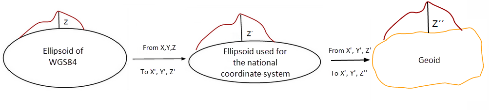","metadata":{}},{"cell_type":"markdown","source":"this is the height, in meters, above the [Reference ellipsoid for World Geodetic System 1984](https://www.mathworks.com/help/map/ref/wgs84ellipsoid.html).\n\nIn the other columns we see\n* `latDeg`, `lngDeg` - The WGS84 latitude, longitude (in decimal degrees) estimated by the reference GNSS receiver (NovAtel SPAN).\n* `timeSinceFirstFixSeconds` - The elapsed time (in seconds) since the first location fix.\n* `hDop` - Horizontal dilution of precision DOP, from the GGA sentence, describes how errors in the measurements affect the final horizontal position estimation.\n* `vDop` - Vertical dilution of precision DOP, from the GSA sentence, describes how errors in the measurements affect the final vertical position estimation.\n* `courseDegree` - The course angle clockwise with respect to the truth north over ground (in degrees).\n* `speedMps` - The speed over ground in meters per second.\n\nOut of curiosity, let us look at the maximum speed","metadata":{}},{"cell_type":"code","source":"max_speed_mps = ground_truth['speedMps'].max()\nmax_speed_mps","metadata":{"trusted":true},"execution_count":null,"outputs":[]},{"cell_type":"markdown","source":"and in miles per hour","metadata":{}},{"cell_type":"code","source":"max_speed_mph = max_speed_mps*3600/1609.344\nmax_speed_mph","metadata":{"trusted":true},"execution_count":null,"outputs":[]},{"cell_type":"markdown","source":"\n## Derived values file","metadata":{}},{"cell_type":"code","source":"derived = pd.read_csv('../input/google-smartphone-decimeter-challenge/train/2021-04-22-US-SJC-1/SamsungS20Ultra//SamsungS20Ultra_derived.csv')\nderived","metadata":{"trusted":true},"execution_count":null,"outputs":[]},{"cell_type":"markdown","source":"from this data we can calculate a *corrected pseudorange*:\n\n> correctedPrM = rawPrM + satClkBiasM - isrbM - ionoDelayM - tropoDelayM\n\nwhere `ionoDelayM` is the ionospheric delay in meters, estimated with the [Klobuchar model](https://gssc.esa.int/navipedia//index.php/Klobuchar_Ionospheric_Model).\nand `tropoDelayM` is the tropospheric delay in meters, estimated with the [EGNOS model](https://doi.org/10.1017/S0373463300001107).\n\n\n","metadata":{}},{"cell_type":"markdown","source":"\n## The test data","metadata":{}},{"cell_type":"code","source":"!ls -1 ../input/google-smartphone-decimeter-challenge/test/","metadata":{"trusted":true},"execution_count":null,"outputs":[]},{"cell_type":"code","source":"!ls -1 ../input/google-smartphone-decimeter-challenge/test/ | wc -w","metadata":{"trusted":true},"execution_count":null,"outputs":[]},{"cell_type":"markdown","source":"we can see that we have 19 directories of test data.\n\n## The haversine and Vincenty formulas\nThe haversine formula is used to calculate the great-circle distance between two points on a sphere, given their longitudes and latitudes. \n\n$$ d = 2r\\arcsin\\left(\\sqrt{hav(\\theta)}\\right) $$\n\nwhere \n\n$$ {hav}(\\theta) = {hav}\\left(\\varphi_2 - \\varphi_1\\right) + \\cos\\left(\\varphi_1\\right)\\cos\\left(\\varphi_2\\right)\\operatorname{hav}\\left(\\lambda_2 - \\lambda_1\\right) $$\n\nwhere $\\varphi$ is the latitude, and $\\lambda$ is the longitude.\n\nHowever, the Earth is not a perfect sphere but rather more like an oblate spheroid, as per the Reference ellipsoid for World Geodetic System of 1984. In view of this Vincenty developed more precise [formulas](https://en.wikipedia.org/wiki/Vincenty%27s_formulae) to take this into account. Despite the complexity of the Vincenty equations there exists a python package, [Vincenty](https://github.com/maurycyp/vincenty) (`!pip install vincenty`) which makes the calculation trivial. ","metadata":{}},{"cell_type":"markdown","source":"\n## Related reading\n* [Guoyu (Michael) Fu, Mohammed Khider, Frank van Diggelen \"*Android Raw GNSS Measurement Datasets for Precise Positioning*\", Proceedings of the 33rd International Technical Meeting of the Satellite Division of The Institute of Navigation (ION GNSS+ 2020) pp. 1925-1937 (2020)](https://doi.org/10.33012/2020.17628)","metadata":{}}]}