{"metadata":{"kernelspec":{"language":"python","display_name":"Python 3","name":"python3"},"language_info":{"pygments_lexer":"ipython3","nbconvert_exporter":"python","version":"3.6.4","file_extension":".py","codemirror_mode":{"name":"ipython","version":3},"name":"python","mimetype":"text/x-python"}},"nbformat_minor":4,"nbformat":4,"cells":[{"cell_type":"markdown","source":"\n\n\nData Mining and Analysis Course Project ( 2021 )
\n\n***\n Team - 5D03
\n\n- [Avantika Shrivastava](https://www.kaggle.com/avantikashrivastava) *- 01FE19BCS253* \n- [Tanmayi Shurpali](https://www.kaggle.com/t01fe19bcs238) *- 01FE19BCS238*\n- [Shrinidhi Kulkarni](https://www.kaggle.com/shrinidhi05) *- 01FE19BCS241* \n- [Bhavana Kumbar](https://www.kaggle.com/bhavanakumbar) *- 01FE19BCS244*\n\n***\n\n## Contents of this Notebok\n1. Imports\n2. Reading DataSet\n3. Explorative Data Analysis\n4. Preprocessing\n5. Model Training\n6. Evaluation\n7. Results and Conclusion\n\n***\n***Kaggle Challange Name:*** [G2Net Gravitational Wave Detection](https://www.kaggle.com/c/g2net-gravitational-wave-detection) - (Submission Deadline : 30th September, 2021)\n***\n***Introduction*** : \n*Gravitational Waves have been discussed since the beginning of the 20th century, and scientifically researched since the Einstein's General Theory of Relativity. They are caused by massive celestial bodies, like the Neutron Stars or ***Black Holes***, when they accelerate they cause gravitational waves, in the form of waves, propagating through the curvature of space-time at the speed of light. These disturbances can be felt on the other side of the observable universe, but are extremely weak as they lose energy as gravitational radiation. It can be imagined similar to throwing a pebble in the pond, the site where the pebble hits water is the source of the disturbance and the outgoing ripples, are the gravitational waves, that get weaker as they move away from the source.In February 2015, the Laser Interferometer Gravitational-wave Observatory ***(LIGO) Scientific Collaboration and the Virgo Collaboration*** announced the first observation of a Gravitational-Wave (GW) signal from a ***stellar-mass Compact Binary Coalescence (CBC) system** .Despite all the initial successes, the future of GW astronomy is facing many challenges. Because of the effectiveness of ML algorithms in identifying patterns in data, ML techniques may be harnessed to make all these searches more sensitive and robust. Applications of ML algorithms to GW searches range from building automated data analysis methods for low-latency pipelines to distinguishing terrestrial noise from astrophysical signals and improving the reach of searches.*\n\n\n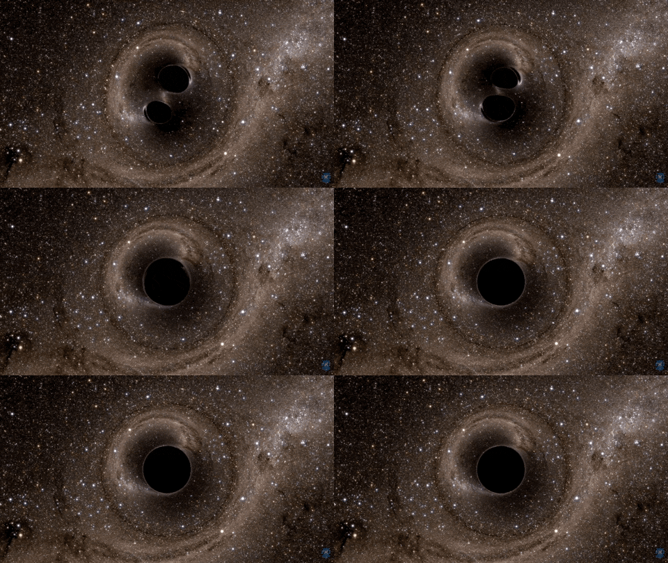\n\n\n***Problem Statement*** : *To preprocess data then build, train & evaluate binary classification model to predict if the given set of signals has Gravitational Waves in them or not.*\n\n***Objectives :*** \n1. *To understand and visulaize raw data using EDA methods*\n2. *To build and train model using Deep Learning Techniques*\n3. *To evaluate model using metrics like ROC AUC (receiver operating charateristics area under curve)*\n\n***\nNote: This notebook was developed and run in the kaggle notebook environment.","metadata":{}},{"cell_type":"markdown","source":"# 1.Imports","metadata":{}},{"cell_type":"code","source":"import numpy as np # linear algebra\nimport pandas as pd # data processing\nimport matplotlib.pyplot as plt # plotting tools\n%matplotlib inline\nimport seaborn as sns\nsns.set()\nplt.rcParams[\"axes.grid\"] = False\n\nimport matplotlib.mlab as mlab\nfrom scipy import signal\nfrom scipy.interpolate import interp1d\nfrom scipy.signal import butter, filtfilt, iirdesign, zpk2tf, freqz\n# Train test split\nfrom sklearn.model_selection import train_test_split\n\nfrom glob import glob\nfrom tqdm import tqdm\n\n# Import tensorflow\nimport tensorflow as tf\n\n# Model & compile arguments\nfrom tensorflow.keras.models import Sequential\nfrom tensorflow.keras.optimizers import Adam\n\n# Get the layers\nfrom tensorflow.keras.layers import Dense\nfrom tensorflow.keras.layers import Conv2D\nfrom tensorflow.keras.layers import MaxPooling2D\nfrom tensorflow.keras.layers import GlobalAveragePooling2D\nfrom tensorflow.keras.layers import Flatten\n\n# Import the Efficientnet models\nfrom tensorflow.keras.applications import EfficientNetB0\n\n# TF model metrics\nfrom tensorflow.keras.metrics import AUC\n\n# \nimport librosa\nimport torch\n\n# (Install &) Import the nnAudio library for Constant Q-Transform\ntry:\n from nnAudio.Spectrogram import CQT1992v2\nexcept:\n !pip install -q nnAudio\n from nnAudio.Spectrogram import CQT1992v2\n#Note: The nnAudio's CQT1992v2 is used, instead of GWpy from analysis notebook, to transform the wave data into Constant Q-Transform spectrograms because this performs the operation much faster and is GPU compatible.\n \nfrom IPython.display import HTML","metadata":{"_kg_hide-input":true,"_kg_hide-output":true,"execution":{"iopub.status.busy":"2021-09-29T14:44:53.949583Z","iopub.execute_input":"2021-09-29T14:44:53.950387Z","iopub.status.idle":"2021-09-29T14:45:12.235404Z","shell.execute_reply.started":"2021-09-29T14:44:53.95035Z","shell.execute_reply":"2021-09-29T14:45:12.234364Z"},"trusted":true},"execution_count":null,"outputs":[]},{"cell_type":"markdown","source":"# 2. Reading Datasets\n\n 1. **train/** - the training set files, one npy file per observation; labels are provided in a files shown below\n 2. **test/** - the test set files; you must predict the probability that the observation contains a gravitational wave\n 3. **training_labels.csv** - target values of whether the associated signal contains a gravitational wave \n 4. **sample_submission.csv** - a sample submission file in the correct format","metadata":{}},{"cell_type":"code","source":"## Get the training ids\ntrain = pd.read_csv('../input/g2net-gravitational-wave-detection/training_labels.csv')\n\n# Get the subsmission file\nsample_sub = pd.read_csv('../input/g2net-gravitational-wave-detection/sample_submission.csv')","metadata":{"execution":{"iopub.status.busy":"2021-09-29T14:45:29.093635Z","iopub.execute_input":"2021-09-29T14:45:29.093983Z","iopub.status.idle":"2021-09-29T14:45:29.824372Z","shell.execute_reply.started":"2021-09-29T14:45:29.093949Z","shell.execute_reply":"2021-09-29T14:45:29.823324Z"},"trusted":true},"execution_count":null,"outputs":[]},{"cell_type":"markdown","source":"# 3. Explorative Data Analysis\n","metadata":{}},{"cell_type":"code","source":"print(f'Training labels: {train.shape[0]} | Test dataset: {sample_sub.shape[0]}')","metadata":{"execution":{"iopub.status.busy":"2021-09-29T05:42:17.204955Z","iopub.execute_input":"2021-09-29T05:42:17.205233Z","iopub.status.idle":"2021-09-29T05:42:17.211084Z","shell.execute_reply.started":"2021-09-29T05:42:17.205207Z","shell.execute_reply":"2021-09-29T05:42:17.210017Z"},"trusted":true},"execution_count":null,"outputs":[]},{"cell_type":"markdown","source":"There are **5,60,000** records in train data and **2,26,000** records in Test data","metadata":{}},{"cell_type":"code","source":"#Checking train data contents\ntrain.head()","metadata":{"execution":{"iopub.status.busy":"2021-09-29T05:42:20.55411Z","iopub.execute_input":"2021-09-29T05:42:20.554596Z","iopub.status.idle":"2021-09-29T05:42:20.573769Z","shell.execute_reply.started":"2021-09-29T05:42:20.554551Z","shell.execute_reply":"2021-09-29T05:42:20.572966Z"},"trusted":true},"execution_count":null,"outputs":[]},{"cell_type":"code","source":"train.shape","metadata":{"execution":{"iopub.status.busy":"2021-09-29T05:42:23.92039Z","iopub.execute_input":"2021-09-29T05:42:23.920907Z","iopub.status.idle":"2021-09-29T05:42:23.927371Z","shell.execute_reply.started":"2021-09-29T05:42:23.920871Z","shell.execute_reply":"2021-09-29T05:42:23.926413Z"},"trusted":true},"execution_count":null,"outputs":[]},{"cell_type":"markdown","source":"- There are **5,60,000 rows** and **2 columns.**\n- The attributes are **'id'** and **'target'**","metadata":{}},{"cell_type":"code","source":"train['target'].value_counts()","metadata":{"execution":{"iopub.status.busy":"2021-09-29T05:42:26.440758Z","iopub.execute_input":"2021-09-29T05:42:26.441076Z","iopub.status.idle":"2021-09-29T05:42:26.457612Z","shell.execute_reply.started":"2021-09-29T05:42:26.441045Z","shell.execute_reply":"2021-09-29T05:42:26.457001Z"},"trusted":true},"execution_count":null,"outputs":[]},{"cell_type":"markdown","source":"**'target'** has value either *'0' or '1'*.","metadata":{}},{"cell_type":"code","source":"train['id'].value_counts()","metadata":{"execution":{"iopub.status.busy":"2021-09-29T05:42:29.936025Z","iopub.execute_input":"2021-09-29T05:42:29.936506Z","iopub.status.idle":"2021-09-29T05:42:30.611007Z","shell.execute_reply.started":"2021-09-29T05:42:29.936455Z","shell.execute_reply":"2021-09-29T05:42:30.610135Z"},"trusted":true},"execution_count":null,"outputs":[]},{"cell_type":"markdown","source":"**'id'** has 5,60,000 unique values.","metadata":{}},{"cell_type":"code","source":"#Checking for any Null Values\ntrain.isnull().sum()","metadata":{"execution":{"iopub.status.busy":"2021-09-29T05:42:33.853288Z","iopub.execute_input":"2021-09-29T05:42:33.853582Z","iopub.status.idle":"2021-09-29T05:42:33.925104Z","shell.execute_reply.started":"2021-09-29T05:42:33.853551Z","shell.execute_reply":"2021-09-29T05:42:33.924187Z"},"trusted":true},"execution_count":null,"outputs":[]},{"cell_type":"markdown","source":"There are no *null* values in the file","metadata":{}},{"cell_type":"code","source":"sns.countplot(data=train, x=\"target\")\n","metadata":{"_kg_hide-input":true,"execution":{"iopub.status.busy":"2021-09-29T05:42:37.941501Z","iopub.execute_input":"2021-09-29T05:42:37.941796Z","iopub.status.idle":"2021-09-29T05:42:38.214938Z","shell.execute_reply.started":"2021-09-29T05:42:37.941763Z","shell.execute_reply":"2021-09-29T05:42:38.214343Z"},"trusted":true},"execution_count":null,"outputs":[]},{"cell_type":"markdown","source":"**Inference**\n- The data is evenly distributed with 50-50 division between the samples with and without gravitational waves signal.\n\n**Insights**\n- The data is binary classified.\n- target *'0'* indicates absence of GW signal i.e **only noise** where as *'1'* indicates presence of GW signal i.e **GW signal + noise.**\n\n## 3.2 Raw Data Visualization\nTo visualize raw signal, we load any one np array file as sample","metadata":{}},{"cell_type":"code","source":"#Obtain path of all 5,60,000 files in ./train\ntrain_path = glob('../input/g2net-gravitational-wave-detection/train/*/*/*/*')","metadata":{"execution":{"iopub.status.busy":"2021-09-29T14:45:42.028021Z","iopub.execute_input":"2021-09-29T14:45:42.028332Z","iopub.status.idle":"2021-09-29T14:48:06.606406Z","shell.execute_reply.started":"2021-09-29T14:45:42.0283Z","shell.execute_reply":"2021-09-29T14:48:06.60548Z"},"trusted":true},"execution_count":null,"outputs":[]},{"cell_type":"code","source":"print(\"The total number of files in the training set:\", len(train_path))","metadata":{"execution":{"iopub.status.busy":"2021-09-29T05:46:23.5442Z","iopub.execute_input":"2021-09-29T05:46:23.544496Z","iopub.status.idle":"2021-09-29T05:46:23.5501Z","shell.execute_reply.started":"2021-09-29T05:46:23.544468Z","shell.execute_reply":"2021-09-29T05:46:23.549171Z"},"trusted":true},"execution_count":null,"outputs":[]},{"cell_type":"code","source":"ids = [path.split(\"/\")[-1].split(\".\")[0] for path in train_path]\npaths_df = pd.DataFrame({\"path\":train_path, \"id\": ids})\ntrain_data = pd.merge(left=train, right=paths_df, on=\"id\")\ntrain_data.head()","metadata":{"_kg_hide-input":true,"execution":{"iopub.status.busy":"2021-09-29T14:49:32.007674Z","iopub.execute_input":"2021-09-29T14:49:32.008018Z","iopub.status.idle":"2021-09-29T14:49:33.372437Z","shell.execute_reply.started":"2021-09-29T14:49:32.007985Z","shell.execute_reply":"2021-09-29T14:49:33.371351Z"},"trusted":true},"execution_count":null,"outputs":[]},{"cell_type":"code","source":"#Load npy files into DataFrame with target 1\nfile_path = pd.DataFrame(train_data).iloc[0]\n\n#Loading any one file\nexample_strain = np.load(file_path.path)","metadata":{"execution":{"iopub.status.busy":"2021-09-29T05:46:33.674474Z","iopub.execute_input":"2021-09-29T05:46:33.674897Z","iopub.status.idle":"2021-09-29T05:46:33.705672Z","shell.execute_reply.started":"2021-09-29T05:46:33.674843Z","shell.execute_reply":"2021-09-29T05:46:33.705007Z"},"trusted":true},"execution_count":null,"outputs":[]},{"cell_type":"code","source":"#View file contents\nprint(example_strain)\n\n#Shape of the array\nprint (example_strain.shape)","metadata":{"execution":{"iopub.status.busy":"2021-09-29T05:46:43.480578Z","iopub.execute_input":"2021-09-29T05:46:43.48104Z","iopub.status.idle":"2021-09-29T05:46:43.51184Z","shell.execute_reply.started":"2021-09-29T05:46:43.481007Z","shell.execute_reply":"2021-09-29T05:46:43.511035Z"},"trusted":true},"execution_count":null,"outputs":[]},{"cell_type":"markdown","source":"**Inference :**\n- There are **3** rows.\n- Each index(row) has **4096** columns.\n\n\n**Insights :**\n- In the competition description it is given that the observations are recorded from 3 gravitational wave interferometers (LIGO Hanford, LIGO Livingston, and Virgo)\n- The quantity in this time series is strain, which is of the order of ~$10^{-20}$, recorded for 2 sec periods sampled at 2048 Hz - 4096 data points.\n- The output of a GW detector is a temporal series of the detector strain, h(t).","metadata":{}},{"cell_type":"code","source":"#Plotting Raw Data from the three detectors\n\ndef plot_graph(example_strain):\n plt.figure(figsize=(20,5))\n\n plt.plot(example_strain[0,:], c=\"firebrick\", label=\"LIGO Hanford\")\n plt.plot(example_strain[1,:], c=\"mediumseagreen\", label=\"LIGO Livingston\")\n plt.plot(example_strain[2,:], c=\"slateblue\", label=\"Virgo\")\n plt.title(\"Id: \"+file_path.id);\n plt.grid(\"on\")\n plt.xlabel(\"Timestamp\");\n plt.legend();","metadata":{"_kg_hide-input":true,"execution":{"iopub.status.busy":"2021-09-29T05:46:48.322654Z","iopub.execute_input":"2021-09-29T05:46:48.323331Z","iopub.status.idle":"2021-09-29T05:46:48.329479Z","shell.execute_reply.started":"2021-09-29T05:46:48.323288Z","shell.execute_reply":"2021-09-29T05:46:48.328679Z"},"trusted":true},"execution_count":null,"outputs":[]},{"cell_type":"code","source":"#Plotting graph for strain with target 1\nplot_graph(example_strain)","metadata":{"_kg_hide-input":true,"execution":{"iopub.status.busy":"2021-09-29T05:46:56.740717Z","iopub.execute_input":"2021-09-29T05:46:56.741431Z","iopub.status.idle":"2021-09-29T05:46:57.161929Z","shell.execute_reply.started":"2021-09-29T05:46:56.741369Z","shell.execute_reply":"2021-09-29T05:46:57.161021Z"},"trusted":true},"execution_count":null,"outputs":[]},{"cell_type":"code","source":"#Load npy files into DataFrame with target 0\nfile_path = pd.DataFrame(train_data).iloc[1]\n\n#Loading any one file\nexample_strain_negative = np.load(file_path.path)\n\n#Plotting graph for strain with target 0\nplot_graph(example_strain_negative)","metadata":{"_kg_hide-input":true,"execution":{"iopub.status.busy":"2021-09-29T05:47:01.04747Z","iopub.execute_input":"2021-09-29T05:47:01.047755Z","iopub.status.idle":"2021-09-29T05:47:01.418292Z","shell.execute_reply.started":"2021-09-29T05:47:01.047727Z","shell.execute_reply":"2021-09-29T05:47:01.417503Z"},"trusted":true},"execution_count":null,"outputs":[]},{"cell_type":"markdown","source":"**Insights**\n- The three signals originating from different detectors all look a bit different.\n- It is difficult to infer just by looking whether the given wave has GW signal or not as there is no notable difference between graphs of *target - 0* and *target - 1.*\n- The strain is of the order $10^{-20}$, which is extremely small and can be affected by many external factors. However, as seen in both the sample plots, the strain data is a combination of many frequencies and analysing the signals in frequency domain, instead of the time domain, might give us better insights.\n- Depending on the location the amplitude recorded varies ( smaller amplitudes indicating *weak signal* detection.\n- Astrophysical signals have typical amplitudes comparable to the detector background noise. Therefore, characterization and reduction of detector noise is essential to GW searches. \n- The interferometer is sensitive towards gravitational waves but unfortunately also for terrestrial forces and displacements.This may also include vibrations of the instruments themselves etc.. This kind of forces cause streching of the interferometer arms and this leads to constructive interferance and the waves we can see above.\n\n### Typical signal processing workflow\nNext, we try to implement the steps from this paper by LIGO by following these steps:\n- Plot the raw signal\n- Window the signal\n- Whiten the signal\n- Bandpass the signal\n\n## Raw Data Visulaization - ASD\nA Fourier Transform is the most commonly used method in maths and signal processing, to decompose the signals into its constituent discrete frequencies. This spectrum of frequencies can be analyzed based on average, power or energy of the signal to get a spectral density plot. As it says, one of the ways to visualize a raw signal in frequency domain is by plotting the amplitude spectral density (ASD).","metadata":{}},{"cell_type":"code","source":"#define some signal parameters\nsample_rate = 2048 #Hz (1/seconds)\ntime_span = 2 # each signal lasts 2 s\nsignal_length = time_span\nsamples_total = time_span * sample_rate\ndt = 1/(samples_total) #4096 points in total\ndt\n\nchannel = 1 #picking detector 1","metadata":{"execution":{"iopub.status.busy":"2021-09-29T05:47:06.492691Z","iopub.execute_input":"2021-09-29T05:47:06.493481Z","iopub.status.idle":"2021-09-29T05:47:06.497741Z","shell.execute_reply.started":"2021-09-29T05:47:06.493446Z","shell.execute_reply":"2021-09-29T05:47:06.497105Z"},"trusted":true},"execution_count":null,"outputs":[]},{"cell_type":"code","source":"# set of observatories\nobs_list = ('LIGO Hanford', 'LIGO Livingston', 'Virgo')","metadata":{"execution":{"iopub.status.busy":"2021-09-29T05:47:10.584918Z","iopub.execute_input":"2021-09-29T05:47:10.58524Z","iopub.status.idle":"2021-09-29T05:47:10.58939Z","shell.execute_reply.started":"2021-09-29T05:47:10.585209Z","shell.execute_reply":"2021-09-29T05:47:10.588536Z"},"trusted":true},"execution_count":null,"outputs":[]},{"cell_type":"code","source":"# Gravitational wave analysis python library\ntry:\n import gwpy\nexcept:\n !pip install -q --user gwpy\n import gwpy\nfrom gwpy.timeseries import TimeSeries","metadata":{"_kg_hide-input":true,"_kg_hide-output":true,"execution":{"iopub.status.busy":"2021-09-29T05:47:13.654861Z","iopub.execute_input":"2021-09-29T05:47:13.655752Z","iopub.status.idle":"2021-09-29T05:47:32.532922Z","shell.execute_reply.started":"2021-09-29T05:47:13.655708Z","shell.execute_reply":"2021-09-29T05:47:32.532085Z"},"trusted":true},"execution_count":null,"outputs":[]},{"cell_type":"code","source":"# function to plot the amplitude spectral density (ASD) plot\ndef plot_asd(sample_id):\n # Get the data\n sample = example_strain\n \n # we convert the data to gwpy's TimeSeries for analysis\n for i in range(sample.shape[0]):\n ts = TimeSeries(sample[i], sample_rate=sample_rate)\n ax = ts.asd(signal_length).plot(figsize=(12, 5)).gca()\n ax.set_xlim(10, 1024);\n ax.set_title(f\"ASD plots for sample: {sample_id} from {obs_list[i]}\");","metadata":{"execution":{"iopub.status.busy":"2021-09-29T05:47:37.657232Z","iopub.execute_input":"2021-09-29T05:47:37.657562Z","iopub.status.idle":"2021-09-29T05:47:37.664571Z","shell.execute_reply.started":"2021-09-29T05:47:37.657529Z","shell.execute_reply":"2021-09-29T05:47:37.66356Z"},"trusted":true},"execution_count":null,"outputs":[]},{"cell_type":"code","source":"# plot ASD for sample w/ GW\nplot_asd(file_path.id)","metadata":{"execution":{"iopub.status.busy":"2021-09-29T05:47:41.37558Z","iopub.execute_input":"2021-09-29T05:47:41.375883Z","iopub.status.idle":"2021-09-29T05:47:45.066072Z","shell.execute_reply.started":"2021-09-29T05:47:41.375828Z","shell.execute_reply":"2021-09-29T05:47:45.065053Z"},"trusted":true},"execution_count":null,"outputs":[]},{"cell_type":"markdown","source":"These plots are plotted on a log scale for x-axis, and we see that it ranges from 10 Hz ~ 1000 Hz. Although, these limits are for visualization purposes only, it helps us see some peaks for each observatory. A particular frequency can be peculiar in one measurement but remember that the GW signal has to be detected in all three waves to be confirmed. This data here still seems a bit noisy and as showed in the tutorial, if sampled for longer periods of time (on real data), it can give some valuable insights. However, the data in this competition is simulated and we try to find other ways to visualize it.\n***\n### Power Spectral Density Plots","metadata":{}},{"cell_type":"code","source":"#Computing Power Series Density\nplt.figure(figsize=(20,5))\n\nfhat = np.fft.fft(example_strain[channel,:], samples_total)\nPSD = fhat * np.conj(fhat) / samples_total\nfreq = 1/(dt*samples_total) * np.arange(samples_total)\n\n\nL = np.arange(1, np.floor(samples_total/2), dtype=\"int\")\nplt.plot(freq[L],PSD[L], '.-')\nplt.grid(\"on\")\nplt.xlabel(\"Frequency Hz\");\nplt.title(\"Power spectral density\");\nplt.yscale(\"log\")","metadata":{"_kg_hide-input":false,"execution":{"iopub.status.busy":"2021-09-29T05:47:59.222055Z","iopub.execute_input":"2021-09-29T05:47:59.222537Z","iopub.status.idle":"2021-09-29T05:47:59.651193Z","shell.execute_reply.started":"2021-09-29T05:47:59.222489Z","shell.execute_reply":"2021-09-29T05:47:59.650283Z"},"trusted":true},"execution_count":null,"outputs":[]},{"cell_type":"markdown","source":"## Insights\n- The steep shape at low frequencies is dominated by noise related to ground motion. \n- Above roughly 100 Hz, the Advanced LIGO detectors are currently quantum noise limited, and their noise curves are dominated by shot noise. \n- High amplitude noise features are also present in the data at certain frequencies, including lines due to the AC power grid (harmonics of 60 Hz in the U.S. and 50 Hz in Europe), mechanical resonances of the mirror suspensions, injected calibration lines, and noise entering through the detector control systems. ","metadata":{}},{"cell_type":"code","source":"#breaking signal into FFT components\nshow_side_effects = True\nfig, ax = plt.subplots(6,1,figsize=(20,15))\n\nax[0].plot(example_strain[channel])\nax[1].plot(np.fft.ifft((PSD>1e-38)*fhat))\nax[2].plot(np.fft.ifft(((PSD>1e-40) & (PSD <= 1e-38))*fhat))\nax[3].plot(np.fft.ifft(((PSD>1e-42) & (PSD <= 1e-40))*fhat))\nax[4].plot(np.fft.ifft(((PSD>0.5e-42) & (PSD <= 1e-42))*fhat))\nax[5].plot(np.fft.ifft((PSD<=0.5e-42)*fhat))\n\nif not show_side_effects:\n for n in range(3,6):\n ax[n].set_xlim(20,2000)","metadata":{"_kg_hide-input":true,"execution":{"iopub.status.busy":"2021-09-29T05:48:04.148817Z","iopub.execute_input":"2021-09-29T05:48:04.149123Z","iopub.status.idle":"2021-09-29T05:48:05.454609Z","shell.execute_reply.started":"2021-09-29T05:48:04.149092Z","shell.execute_reply":"2021-09-29T05:48:05.453807Z"},"trusted":true},"execution_count":null,"outputs":[]},{"cell_type":"markdown","source":"- The first step in many LVC analyses is to Fourier transform the time-domain data using a fast Fourier transform (FFT) . - - There are interesting kind of side effects in the beginning and the end of each wave after doing the inverse Fourier transform.\n- Since the FFT implicitly assumes that the stretch of data being transformed is periodic in time, window functions have to be applied to the data to suppress spectral leakage using e.g. a Tukey (cosine-tapered) window function. \n- Failing to window the data will lead to spectral leakage and spurious correlations in the phase between bins. \n\n### Apply Window Functions - Removing Spectral leakages","metadata":{}},{"cell_type":"code","source":"from scipy import signal\nfrom scipy.interpolate import interp1d\nfrom scipy.signal import butter, filtfilt, iirdesign, zpk2tf, freqz","metadata":{"_kg_hide-input":true,"execution":{"iopub.status.busy":"2021-09-29T05:48:10.495677Z","iopub.execute_input":"2021-09-29T05:48:10.496249Z","iopub.status.idle":"2021-09-29T05:48:10.501161Z","shell.execute_reply.started":"2021-09-29T05:48:10.496206Z","shell.execute_reply":"2021-09-29T05:48:10.50005Z"},"trusted":true},"execution_count":null,"outputs":[]},{"cell_type":"code","source":"hp_window = 1\nhp_tukey_alpha = 0.125\nfband = [35.0, 200.0]","metadata":{"_kg_hide-input":true,"execution":{"iopub.status.busy":"2021-09-29T05:48:17.551091Z","iopub.execute_input":"2021-09-29T05:48:17.551388Z","iopub.status.idle":"2021-09-29T05:48:17.55626Z","shell.execute_reply.started":"2021-09-29T05:48:17.551357Z","shell.execute_reply":"2021-09-29T05:48:17.55528Z"},"trusted":true},"execution_count":null,"outputs":[]},{"cell_type":"code","source":"blackman_window = signal.blackman(int(samples_total*hp_window)) #signal.tukey(strain, alpha=1./8)\ntukey_window = signal.tukey(samples_total*hp_window, hp_tukey_alpha)","metadata":{"execution":{"iopub.status.busy":"2021-09-29T05:48:25.057581Z","iopub.execute_input":"2021-09-29T05:48:25.057893Z","iopub.status.idle":"2021-09-29T05:48:25.064192Z","shell.execute_reply.started":"2021-09-29T05:48:25.057835Z","shell.execute_reply":"2021-09-29T05:48:25.063254Z"},"trusted":true},"execution_count":null,"outputs":[]},{"cell_type":"code","source":"fig, ax = plt.subplots(3,1,figsize=(20,15))\n\n#plotting raw data\nax[0].plot(example_strain[channel])\nax[0].set_title(\"Original data\")\n\n#plotting data with blackman \nax[1].plot(example_strain[channel]*blackman_window)\nax[1].set_title(\"With blackman window applied\")\n\n#plotting data with tukey window\nax[2].plot(example_strain[channel]*tukey_window)\nax[2].set_title(\"With tukey window applied\");","metadata":{"_kg_hide-input":true,"execution":{"iopub.status.busy":"2021-09-29T05:48:28.72461Z","iopub.execute_input":"2021-09-29T05:48:28.72527Z","iopub.status.idle":"2021-09-29T05:48:29.565312Z","shell.execute_reply.started":"2021-09-29T05:48:28.72523Z","shell.execute_reply":"2021-09-29T05:48:29.564427Z"},"trusted":true},"execution_count":null,"outputs":[]},{"cell_type":"markdown","source":"For the analysis of transient data the use of **Tukey windows** is advantageous as signals will suffer less modification than, **Blackman windows**.","metadata":{}},{"cell_type":"code","source":"windowed_strain = example_strain[channel]*tukey_window","metadata":{"_kg_hide-input":true,"execution":{"iopub.status.busy":"2021-09-29T05:48:34.452058Z","iopub.execute_input":"2021-09-29T05:48:34.452357Z","iopub.status.idle":"2021-09-29T05:48:34.456933Z","shell.execute_reply.started":"2021-09-29T05:48:34.452326Z","shell.execute_reply":"2021-09-29T05:48:34.456004Z"},"trusted":true},"execution_count":null,"outputs":[]},{"cell_type":"markdown","source":"### Whitening - Making signal more Uniform\n\n- Whitening the data is suppressing the extra noise at low frequencies and at the spectral lines, to better see the weak signals in the most sensitive band.\n- It is always one of the first steps in astrophysical data analysis (searches, parameter estimation).\n- It requires no prior knowledge of spectral lines, etc; only the data are needed.","metadata":{}},{"cell_type":"code","source":"#Whitening data to make signal more uniform\ndef whiten(strain, samples_total, dt):\n # TODO: normalization \n \n fhat = np.fft.fft(strain, samples_total)\n PSD = fhat * np.conj(fhat) / samples_total\n freq = 1/(dt*samples_total) * np.arange(samples_total)\n \n # scipy interp1d interpolation\n interp_psd = interp1d(freq, PSD, \"nearest\")\n \n w_fhat = fhat/np.sqrt(interp_psd(freq))\n w_strain = np.fft.ifft(w_fhat)\n return w_strain, interp_psd(freq)","metadata":{"_kg_hide-input":true,"execution":{"iopub.status.busy":"2021-09-29T05:48:46.318607Z","iopub.execute_input":"2021-09-29T05:48:46.318929Z","iopub.status.idle":"2021-09-29T05:48:46.327297Z","shell.execute_reply.started":"2021-09-29T05:48:46.318896Z","shell.execute_reply":"2021-09-29T05:48:46.325697Z"},"trusted":true},"execution_count":null,"outputs":[]},{"cell_type":"code","source":"w_strain, ip = whiten(windowed_strain, samples_total, dt)","metadata":{"_kg_hide-input":true,"execution":{"iopub.status.busy":"2021-09-29T05:48:50.497611Z","iopub.execute_input":"2021-09-29T05:48:50.497931Z","iopub.status.idle":"2021-09-29T05:48:50.505619Z","shell.execute_reply.started":"2021-09-29T05:48:50.497893Z","shell.execute_reply":"2021-09-29T05:48:50.50483Z"},"trusted":true},"execution_count":null,"outputs":[]},{"cell_type":"code","source":"#plotting whitened data\nfig, ax = plt.subplots(2,1,figsize=(20,10))\nax[0].plot(np.log(ip[0:1024]), '-o')\nax[0].set_title(\"Interpolated PSD\")\nax[0].set_xlabel(\"Frequency Hz\")\nax[0].set_ylabel(\"Sn(t)\")\nax[1].plot(w_strain, '-.')\nax[1].set_ylabel(\"dw(t)\")\nax[1].set_xlabel(\"Timestamp\")\n","metadata":{"_kg_hide-input":true,"execution":{"iopub.status.busy":"2021-09-29T05:48:59.470714Z","iopub.execute_input":"2021-09-29T05:48:59.471028Z","iopub.status.idle":"2021-09-29T05:49:00.598953Z","shell.execute_reply.started":"2021-09-29T05:48:59.47099Z","shell.execute_reply":"2021-09-29T05:49:00.598022Z"},"trusted":true},"execution_count":null,"outputs":[]},{"cell_type":"markdown","source":"This is the whitened signal. Next, since we know this data is from merger binary black holes, the frequency is in lower range and this we apply a bandpass filter to passthrough signals between 35 ~ 350 Hz.\n***\n### Bandpass Filter - Filtering signal for certain bandwidth","metadata":{}},{"cell_type":"code","source":"#Defining bandpass filter\ndef bandpass(strain, fband, fs):\n \"\"\"Bandpasses strain data using a butterworth filter.\n \n Args:\n strain (ndarray): strain data to bandpass\n fband (ndarray): low and high-pass filter values to use\n fs (float): sample rate of data\n \n Returns:\n ndarray: array of bandpassed strain data\n \"\"\"\n bb, ab = butter(4, [fband[0]*2./fs, fband[1]*2./fs], btype='band')\n normalization = np.sqrt((fband[1]-fband[0])/(fs/2))\n strain_bp = filtfilt(bb, ab, strain) / normalization\n return strain_bp\n\n#Applying bandpass filter\nbandpassed_strain = bandpass(w_strain, fband, samples_total)\n\n#plotting bandpass filtered data\nplt.figure(figsize=(20,5))\nplt.plot(bandpassed_strain, '-')","metadata":{"execution":{"iopub.status.busy":"2021-09-29T05:49:04.762842Z","iopub.execute_input":"2021-09-29T05:49:04.763163Z","iopub.status.idle":"2021-09-29T05:49:05.145919Z","shell.execute_reply.started":"2021-09-29T05:49:04.763132Z","shell.execute_reply":"2021-09-29T05:49:05.144939Z"},"trusted":true},"execution_count":null,"outputs":[]},{"cell_type":"markdown","source":"**Constant Q-Transform**\n- The signal analysis didn't provide much insights, so let's try the second method in signal processing. Tranforming the waves into spectrograms images, i.e. frequency-domain, and then visualize them. This technique is widely used in audio analysis and since our data is a wave with bunch of frequencies, we can use the same technique as well.\n- The advantage of using a spectrogram, over a direct Fourier Transform where you lose time info, is that it captures the shift or change in frequencies over time and this removes white noise frequencies that are persistent, leaving the signals of interest. Constant Q-Transform is one way to visualize the spectrogram.","metadata":{}},{"cell_type":"code","source":"# function to plot the Q-transform spectrogram\ndef plot_q_transform(sample_id,example_strain):\n # Get the data\n sample = example_strain\n \n # we convert the data to gwpy's TimeSeries for analysis\n for i in range(sample.shape[0]):\n ts = TimeSeries(sample[i], sample_rate=sample_rate)\n ax = ts.q_transform(whiten=True).plot().gca()\n ax.set_xlabel('')\n ax.set_title(f\"Spectrogram plots for sample: {sample_id} from {obs_list[i]}\")\n ax.grid(False)\n ax.set_yscale('log');","metadata":{"execution":{"iopub.status.busy":"2021-09-29T05:49:10.537495Z","iopub.execute_input":"2021-09-29T05:49:10.537787Z","iopub.status.idle":"2021-09-29T05:49:10.544212Z","shell.execute_reply.started":"2021-09-29T05:49:10.53776Z","shell.execute_reply":"2021-09-29T05:49:10.543374Z"},"trusted":true},"execution_count":null,"outputs":[]},{"cell_type":"code","source":"# plot the Q-transform for sample w/ GW\nplot_q_transform(file_path.id,example_strain)","metadata":{"execution":{"iopub.status.busy":"2021-09-29T05:49:13.796445Z","iopub.execute_input":"2021-09-29T05:49:13.79675Z","iopub.status.idle":"2021-09-29T05:49:28.866369Z","shell.execute_reply.started":"2021-09-29T05:49:13.796717Z","shell.execute_reply":"2021-09-29T05:49:28.865774Z"},"trusted":true},"execution_count":null,"outputs":[]},{"cell_type":"markdown","source":"- Visibly, all three signals have different features and the above were plotted from a sample which has gravitational waves, and it shows the famous 'chirp' confirming the presence of gravitational waves. \n- This transformation removes the unwanted noise frequencies, but still some of it remains, but a signal has to be detected in all three waves to be predicted as gravitational wave.\n- Next, we can compare how the Q-Transforms look for samples with and without gravitational wave signals.","metadata":{}},{"cell_type":"code","source":"sample_gw_id = pd.DataFrame(train_data).iloc[0].id\nsample_no_gw_id = pd.DataFrame(train_data).iloc[1].id\n\n# function to plot the Q-transform spectrogram side-by-side\ndef plot_q_transform_sbs(sample_gw_id, sample_no_gw_id,example_strain,example_strain_negative ):\n # Get the data\n sample_gw = example_strain\n sample_no_gw = example_strain_negative\n \n for i in range(len(obs_list)):\n # get the timeseries\n ts_gw = TimeSeries(sample_gw[i], sample_rate=sample_rate)\n ts_no_gw = TimeSeries(sample_no_gw[i], sample_rate=sample_rate)\n \n # get the Q-transform\n image_gw = ts_gw.q_transform(whiten=True)\n image_no_gw = ts_no_gw.q_transform(whiten=True)\n\n plt.figure(figsize=(20, 10))\n plt.subplot(131)\n plt.imshow(image_gw)\n plt.title(f\"id: {sample_gw_id} | Target=1\")\n plt.grid(False)\n\n plt.subplot(132)\n plt.imshow(image_no_gw)\n plt.title(f\"id: {sample_no_gw_id} | Target=0\")\n plt.grid(False)\n \n plt.show()\n","metadata":{"execution":{"iopub.status.busy":"2021-09-29T05:49:35.531439Z","iopub.execute_input":"2021-09-29T05:49:35.531716Z","iopub.status.idle":"2021-09-29T05:49:35.542423Z","shell.execute_reply.started":"2021-09-29T05:49:35.53169Z","shell.execute_reply":"2021-09-29T05:49:35.54149Z"},"trusted":true},"execution_count":null,"outputs":[]},{"cell_type":"code","source":"# let's plot two spectrograms for sample w/ and w/o GW signal side-by-side\nplot_q_transform_sbs(sample_gw_id, sample_no_gw_id,example_strain,example_strain_negative )","metadata":{"execution":{"iopub.status.busy":"2021-09-29T05:49:41.906113Z","iopub.execute_input":"2021-09-29T05:49:41.906983Z","iopub.status.idle":"2021-09-29T05:49:44.783481Z","shell.execute_reply.started":"2021-09-29T05:49:41.906931Z","shell.execute_reply":"2021-09-29T05:49:44.782548Z"},"trusted":true},"execution_count":null,"outputs":[]},{"cell_type":"markdown","source":"- Apart from a few hints, we cannot say for sure that the difference between the waves with and without GW signals is obvious. \n- There can be some cleaning or filtering we can apply to remove the noise further but that's where the Deep Learning shines. \n- The things we can't detect visually, machine learning can. Next, in the modelling notebook, we build data pipelines, transform the data to spectrograms, and build models to make the predictions.\n***\n\n# 4.Preprocessing Methods\nAstrophysical signals have typical amplitudes comparable to the detector background noise. Therefore, characterization and reduction of detector noise is essential to GW searches. \nWe follow signal processing methodology to preprocess signals, converting the time domain data to frequency domain, converting to Constant Q-Transform images and using these as input to our model training step. \n\nThere are mainly two ways in which we can preprocess this type of data to train our models:\n\n1. **Using the time series data,** and performing some cleaning steps to enhance the signal, remove noise, as described in publications by B P Abbott et al. and Daniel George et al.Typical signal processing workflow\nNext, we try to implement the steps from this paper referenced above by following these steps:\nPlot the raw signal\nWindow the signal\nWhiten the signal\nBandpass the signal\n1. **Getting the Constant Q-Transformed spectrogram image,** which is a frequency-domain fourier transformed data, while treating the sample being analyzed as a wave.","metadata":{}},{"cell_type":"markdown","source":"**Creating TF Data pipeline :**\nNext, we create the TensorFlow input data pipeline. This is crucial as loading such a huge dataset can create a bottleneck on the entire workflow and can cause memory overload.","metadata":{}},{"cell_type":"code","source":"# function to return the npy file corresponding to the id\ndef get_npy_filepath(id_, is_train=True):\n path = ''\n if is_train:\n return f'../input/g2net-gravitational-wave-detection/train/{id_[0]}/{id_[1]}/{id_[2]}/{id_}.npy'\n else:\n return f'../input/g2net-gravitational-wave-detection/test/{id_[0]}/{id_[1]}/{id_[2]}/{id_}.npy'","metadata":{"execution":{"iopub.status.busy":"2021-09-29T14:50:01.970801Z","iopub.execute_input":"2021-09-29T14:50:01.971145Z","iopub.status.idle":"2021-09-29T14:50:01.976741Z","shell.execute_reply.started":"2021-09-29T14:50:01.9711Z","shell.execute_reply":"2021-09-29T14:50:01.975783Z"},"trusted":true},"execution_count":null,"outputs":[]},{"cell_type":"code","source":"# let's define some signal parameters\nsample_rate = 2048 # data is provided at 2048 Hz\nsignal_length = 2 # each signal lasts 2 s\nfmin, fmax = 20, 1024 # filter above 20 Hz, and max 1024 Hz (Nyquist freq = sample_rate/2)\nhop_length = 64 # hop length parameter for the stft\n\n# model compile params\nbatch_size = 250 # size in which data is processed and trained at-once in model\nepochs = 3 # number of epochs (keep low as dataset is quite large 3~5 is enough as observed)","metadata":{"execution":{"iopub.status.busy":"2021-09-29T14:50:05.736659Z","iopub.execute_input":"2021-09-29T14:50:05.736956Z","iopub.status.idle":"2021-09-29T14:50:05.742154Z","shell.execute_reply.started":"2021-09-29T14:50:05.736928Z","shell.execute_reply":"2021-09-29T14:50:05.741253Z"},"trusted":true},"execution_count":null,"outputs":[]},{"cell_type":"code","source":"# Define the Constant Q-Transform\ntransform = CQT1992v2(sr=sample_rate, fmin=fmin, fmax=fmax, hop_length=hop_length)\n\n# check if GPU enabled, then run the transform on GPU for faster execution\n# if tf.test.is_gpu_available():\n# cq_transform = cq_transform.to('cuda')","metadata":{"execution":{"iopub.status.busy":"2021-09-29T14:50:14.01351Z","iopub.execute_input":"2021-09-29T14:50:14.013995Z","iopub.status.idle":"2021-09-29T14:50:14.067958Z","shell.execute_reply.started":"2021-09-29T14:50:14.013952Z","shell.execute_reply":"2021-09-29T14:50:14.067298Z"},"trusted":true},"execution_count":null,"outputs":[]},{"cell_type":"code","source":"# function to load the file, preprocess, return the respective Constant Q-transform\n# the Cqt function\n# preprocess function\ndef preprocess_function_cqt(path):\n signal = np.load(path.numpy())\n # there are 3 signal as explained before for each interferometers\n for i in range(signal.shape[0]):\n # normalize signal\n signal[i] /= np.max(signal[i])\n # horizontal stack\n signal = np.hstack(signal)\n # tensor conversion\n signal = torch.from_numpy(signal).float()\n # getting the image from CQT transform\n image = transform(signal)\n # converting to array from tensor\n image = np.array(image)\n # transpose the image to get right orientation\n image = np.transpose(image,(1,2,0))\n \n # conver the image to tf.tensor and return\n return tf.convert_to_tensor(image)","metadata":{"execution":{"iopub.status.busy":"2021-09-29T14:50:20.542813Z","iopub.execute_input":"2021-09-29T14:50:20.543249Z","iopub.status.idle":"2021-09-29T14:50:20.55153Z","shell.execute_reply.started":"2021-09-29T14:50:20.543216Z","shell.execute_reply":"2021-09-29T14:50:20.550733Z"},"trusted":true},"execution_count":null,"outputs":[]},{"cell_type":"code","source":"image = preprocess_function_cqt(tf.convert_to_tensor(train_data['path'][2]))\nprint(image.shape)\nplt.imshow(image)","metadata":{"execution":{"iopub.status.busy":"2021-09-29T05:50:10.495982Z","iopub.execute_input":"2021-09-29T05:50:10.496888Z","iopub.status.idle":"2021-09-29T05:50:11.039497Z","shell.execute_reply.started":"2021-09-29T05:50:10.496826Z","shell.execute_reply":"2021-09-29T05:50:11.038666Z"},"trusted":true},"execution_count":null,"outputs":[]},{"cell_type":"code","source":"# From the Constant Q-Transform that we got, get the shape\ninput_shape = (69, 193, 1)","metadata":{"execution":{"iopub.status.busy":"2021-09-29T14:50:33.18284Z","iopub.execute_input":"2021-09-29T14:50:33.183188Z","iopub.status.idle":"2021-09-29T14:50:33.188446Z","shell.execute_reply.started":"2021-09-29T14:50:33.183155Z","shell.execute_reply":"2021-09-29T14:50:33.187572Z"},"trusted":true},"execution_count":null,"outputs":[]},{"cell_type":"markdown","source":"***\n# 5. Modeling\n**Strategy**\n\n- This is essentially a signal processing problem with classification task, there can be two ways in which we can build models around this data, as also mentioned in the [LIGO research paper](https://arxiv.org/pdf/1908.11170.pdf) - using \"raw\" signals with minimal pre-processing and using \"images\" by transforming the waves into spectrograms. \n- However, building models on raw signal data, by following the cleaning steps from respective publications, didnot yield acceptable results. It is worth mentioning that only a part of the data was used while strategy selection process, and it was concluded that more pre-processing was necessary, or rather proper pre-processing, if we were to use raw signal.\n- Eventually, the second method that we went with in this project, is used to transform the waves into the spectrogram image. We train two models to evaluate the results:\n1. Simple CNN- a simple CNN architecture that is a modified version of the model usually used in MNIST Digit Recognizer tutorials. This acts as our baseline model.\n2. EfficientNet-a EfficientNetB7 model that has been developed and pre-trained on ImageNet dataset. This model is chosen as it is known for its excellent performance with significantly fewer number of parameters, that can drastically improve the computational efficiency.","metadata":{}},{"cell_type":"code","source":"# Get the feature ids and target\nX = train_data['id']\ny = train_data['target'].astype('int8').values","metadata":{"execution":{"iopub.status.busy":"2021-09-29T14:50:37.790963Z","iopub.execute_input":"2021-09-29T14:50:37.791528Z","iopub.status.idle":"2021-09-29T14:50:37.798358Z","shell.execute_reply.started":"2021-09-29T14:50:37.791483Z","shell.execute_reply":"2021-09-29T14:50:37.797521Z"},"trusted":true},"execution_count":null,"outputs":[]},{"cell_type":"code","source":"x_train, x_valid, y_train, y_valid = train_test_split(X, y, random_state = 51, stratify = y)","metadata":{"execution":{"iopub.status.busy":"2021-09-29T14:50:42.535224Z","iopub.execute_input":"2021-09-29T14:50:42.53575Z","iopub.status.idle":"2021-09-29T14:50:43.017353Z","shell.execute_reply.started":"2021-09-29T14:50:42.535715Z","shell.execute_reply":"2021-09-29T14:50:43.016678Z"},"trusted":true},"execution_count":null,"outputs":[]},{"cell_type":"code","source":"def preprocess_function_parse_tf(path, y=None):\n [x] = tf.py_function(func=preprocess_function_cqt, inp=[path], Tout=[tf.float32])\n x = tf.ensure_shape(x, input_shape)\n if y is None:\n return x\n else:\n return x,y","metadata":{"execution":{"iopub.status.busy":"2021-09-29T14:50:49.813684Z","iopub.execute_input":"2021-09-29T14:50:49.814036Z","iopub.status.idle":"2021-09-29T14:50:49.819147Z","shell.execute_reply.started":"2021-09-29T14:50:49.814008Z","shell.execute_reply":"2021-09-29T14:50:49.818547Z"},"trusted":true},"execution_count":null,"outputs":[]},{"cell_type":"code","source":"train_dataset = tf.data.Dataset.from_tensor_slices((x_train.apply(get_npy_filepath).values, y_train))\n# shuffle the dataset\ntrain_dataset = train_dataset.shuffle(len(x_train))\ntrain_dataset = train_dataset.map(preprocess_function_parse_tf, num_parallel_calls=tf.data.AUTOTUNE)\ntrain_dataset = train_dataset.batch(batch_size)\ntrain_dataset = train_dataset.prefetch(tf.data.AUTOTUNE)","metadata":{"execution":{"iopub.status.busy":"2021-09-29T14:50:53.186844Z","iopub.execute_input":"2021-09-29T14:50:53.187775Z","iopub.status.idle":"2021-09-29T14:50:53.836518Z","shell.execute_reply.started":"2021-09-29T14:50:53.187729Z","shell.execute_reply":"2021-09-29T14:50:53.835509Z"},"_kg_hide-output":true,"trusted":true},"execution_count":null,"outputs":[]},{"cell_type":"code","source":"# valid dataset\n# Get the data filepaths as tensor_slices\nvalid_dataset = tf.data.Dataset.from_tensor_slices((x_valid.apply(get_npy_filepath).values, y_valid))\n\n# apply the map method to tf_parse_function()\nvalid_dataset = valid_dataset.map(preprocess_function_parse_tf, num_parallel_calls=tf.data.AUTOTUNE)\n\n# set batch size of the dataset\nvalid_dataset = valid_dataset.batch(batch_size)\n\n# prefetch the data\nvalid_dataset = valid_dataset.prefetch(tf.data.AUTOTUNE)\n","metadata":{"execution":{"iopub.status.busy":"2021-09-29T14:51:02.469151Z","iopub.execute_input":"2021-09-29T14:51:02.469435Z","iopub.status.idle":"2021-09-29T14:51:02.632708Z","shell.execute_reply.started":"2021-09-29T14:51:02.469398Z","shell.execute_reply":"2021-09-29T14:51:02.632053Z"},"trusted":true},"execution_count":null,"outputs":[]},{"cell_type":"markdown","source":"## 1. Baseline Model : Simple CNN","metadata":{}},{"cell_type":"code","source":"#CNN Modeling\ntrain_dataset.take(1)\n\n#Instantiate the Sequential model\nmodel_cnn = Sequential(name='CNN_model')\n\n# Add the first Convoluted2D layer w/ input_shape & MaxPooling2D layer followed by that\nmodel_cnn.add(Conv2D(filters=16,\n kernel_size=3,\n input_shape=input_shape,\n activation='relu',\n name='Conv_01'))\nmodel_cnn.add(MaxPooling2D(pool_size=2, name='Pool_01'))\n\n# Second pair of Conv1D and MaxPooling1D layers\nmodel_cnn.add(Conv2D(filters=32,\n kernel_size=3,\n input_shape=input_shape,\n activation='relu',\n name='Conv_02'))\nmodel_cnn.add(MaxPooling2D(pool_size=2, name='Pool_02'))\n\n# Third pair of Conv1D and MaxPooling1D layers\nmodel_cnn.add(Conv2D(filters=64,\n kernel_size=3,\n input_shape=input_shape,\n activation='relu',\n name='Conv_03'))\nmodel_cnn.add(MaxPooling2D(pool_size=2, name='Pool_03'))\n\n# Add the Flatten layer\nmodel_cnn.add(Flatten(name='Flatten'))\n\n# Add the Dense layers\nmodel_cnn.add(Dense(units=512,\n activation='relu',\n name='Dense_01'))\nmodel_cnn.add(Dense(units=64,\n activation='relu',\n name='Dense_02'))\n\n# Add the final Output layer\nmodel_cnn.add(Dense(1, activation='sigmoid', name='Output'))","metadata":{"execution":{"iopub.status.busy":"2021-09-29T14:51:15.11636Z","iopub.execute_input":"2021-09-29T14:51:15.117272Z","iopub.status.idle":"2021-09-29T14:51:15.275891Z","shell.execute_reply.started":"2021-09-29T14:51:15.117217Z","shell.execute_reply":"2021-09-29T14:51:15.274766Z"},"trusted":true},"execution_count":null,"outputs":[]},{"cell_type":"code","source":"# Display the CNN model architecture\nmodel_cnn.summary()","metadata":{"execution":{"iopub.status.busy":"2021-09-29T14:51:19.216521Z","iopub.execute_input":"2021-09-29T14:51:19.216799Z","iopub.status.idle":"2021-09-29T14:51:19.22676Z","shell.execute_reply.started":"2021-09-29T14:51:19.216772Z","shell.execute_reply":"2021-09-29T14:51:19.226039Z"},"trusted":true},"execution_count":null,"outputs":[]},{"cell_type":"code","source":"# compile the model with following parameters\n# Optimizer: Adam (learning_rate=0.0001)\n# loss: binary_crossentropy\n# metrics: accuracy/AUC\nmodel_cnn.compile(optimizer=Adam(learning_rate=0.0001),\n loss='binary_crossentropy',\n metrics=[[AUC(), 'accuracy']])\n\n# Fit the data\nhistory_cnn = model_cnn.fit(x=train_dataset,\n epochs=3,\n validation_data=valid_dataset,\n batch_size=batch_size,\n verbose=1)","metadata":{},"execution_count":null,"outputs":[]},{"cell_type":"markdown","source":"- The baseline model seems to be converging well only after about 3 epochs. \n- But, it takes almost about an hour to train each epoch, we can only say that the model can be improved with further training and fine-tuning the structure. \n- At the end of 3rd epoch, we see 0.83 AUC score and 0.76 accuracy for training dataset, while 0.84 AUC score and 0.77 accuracy for the validation dataset.","metadata":{}},{"cell_type":"code","source":"# save the model\nmodel_cnn.save('./model_CNN.h5')","metadata":{"execution":{"iopub.status.busy":"2021-09-29T04:43:23.353314Z","iopub.status.idle":"2021-09-29T04:43:23.353657Z","shell.execute_reply.started":"2021-09-29T04:43:23.353466Z","shell.execute_reply":"2021-09-29T04:43:23.353488Z"},"trusted":true},"execution_count":null,"outputs":[]},{"cell_type":"code","source":"sub = pd.read_csv('../input/g2net-gravitational-wave-detection/sample_submission.csv')\nx_test = sub[['id']]","metadata":{"execution":{"iopub.status.busy":"2021-09-29T14:51:41.109855Z","iopub.execute_input":"2021-09-29T14:51:41.110625Z","iopub.status.idle":"2021-09-29T14:51:41.302194Z","shell.execute_reply.started":"2021-09-29T14:51:41.110577Z","shell.execute_reply":"2021-09-29T14:51:41.30139Z"},"trusted":true},"execution_count":null,"outputs":[]},{"cell_type":"code","source":"x_test.tail()","metadata":{"execution":{"iopub.status.busy":"2021-09-29T14:51:47.170681Z","iopub.execute_input":"2021-09-29T14:51:47.171197Z","iopub.status.idle":"2021-09-29T14:51:47.180125Z","shell.execute_reply.started":"2021-09-29T14:51:47.171158Z","shell.execute_reply":"2021-09-29T14:51:47.178989Z"},"trusted":true},"execution_count":null,"outputs":[]},{"cell_type":"code","source":"# test dataset\ntest_dataset = tf.data.Dataset.from_tensor_slices((x_test['id'].apply(get_npy_filepath, is_train=False).values))\ntest_dataset = test_dataset.map(preprocess_function_parse_tf, num_parallel_calls=tf.data.AUTOTUNE)\ntest_dataset = test_dataset.batch(batch_size)\ntest_dataset = test_dataset.prefetch(tf.data.AUTOTUNE)","metadata":{"execution":{"iopub.status.busy":"2021-09-29T14:51:52.637725Z","iopub.execute_input":"2021-09-29T14:51:52.638036Z","iopub.status.idle":"2021-09-29T14:51:52.908141Z","shell.execute_reply.started":"2021-09-29T14:51:52.638004Z","shell.execute_reply":"2021-09-29T14:51:52.907146Z"},"trusted":true},"execution_count":null,"outputs":[]},{"cell_type":"markdown","source":"The Simple CNN model has been trained and can be found in our this version of [Notebook](https://www.kaggle.com/t01fe19bcs238/g2net-eda-preprocessing-model) ","metadata":{}},{"cell_type":"code","source":"# load the trained Simple CNN model \nsaved_cnn_model = tf.keras.models.load_model('../input/g2netfinal/full_cnn_model.h5')","metadata":{"execution":{"iopub.status.busy":"2021-09-29T14:52:01.285946Z","iopub.execute_input":"2021-09-29T14:52:01.286235Z","iopub.status.idle":"2021-09-29T14:52:03.22983Z","shell.execute_reply.started":"2021-09-29T14:52:01.286207Z","shell.execute_reply":"2021-09-29T14:52:03.228788Z"},"trusted":true},"execution_count":null,"outputs":[]},{"cell_type":"code","source":"saved_cnn_model.fit(x=valid_dataset, epochs=3, batch_size=batch_size, verbose=1)","metadata":{"execution":{"iopub.status.busy":"2021-09-29T14:52:06.646311Z","iopub.execute_input":"2021-09-29T14:52:06.646585Z","iopub.status.idle":"2021-09-29T15:54:28.939992Z","shell.execute_reply.started":"2021-09-29T14:52:06.646557Z","shell.execute_reply":"2021-09-29T15:54:28.935487Z"},"trusted":true},"execution_count":null,"outputs":[]},{"cell_type":"code","source":"saved_cnn_model.save('./model/full_cnn_model.h5')","metadata":{"execution":{"iopub.status.busy":"2021-09-29T04:43:23.362835Z","iopub.status.idle":"2021-09-29T04:43:23.363171Z","shell.execute_reply.started":"2021-09-29T04:43:23.362997Z","shell.execute_reply":"2021-09-29T04:43:23.363017Z"},"trusted":true},"execution_count":null,"outputs":[]},{"cell_type":"code","source":"full_cnn_model = tf.keras.models.load_model('./model/full_cnn_model.h5')","metadata":{"execution":{"iopub.status.busy":"2021-09-29T04:43:23.364108Z","iopub.status.idle":"2021-09-29T04:43:23.364438Z","shell.execute_reply.started":"2021-09-29T04:43:23.364259Z","shell.execute_reply":"2021-09-29T04:43:23.364281Z"},"trusted":true},"execution_count":null,"outputs":[]},{"cell_type":"code","source":"# predict the test dataset using CNN\npreds_cnn = saved_cnn_model.predict(test_dataset)","metadata":{"trusted":true},"execution_count":null,"outputs":[]},{"cell_type":"code","source":"# Function to save kaggle submissions for test prediction probabilities\ndef get_kaggle_format(prediction_probs, model='base'):\n # load the sample submission file\n# sub = pd.read_csv('../input/g2net-gravitational-wave-detection/sample_submission.csv')\n sample_sub['target'] = prediction_probs\n \n # Output filename for kaggle submission\n filename = f\"kaggle_sub_{model}.csv\"\n \n # Save the DataFrame to a file\n sample_sub.to_csv(filename, index=False)\n print(f'File name: {filename}')","metadata":{"execution":{"iopub.status.busy":"2021-09-29T05:59:53.68413Z","iopub.execute_input":"2021-09-29T05:59:53.684446Z","iopub.status.idle":"2021-09-29T05:59:53.690107Z","shell.execute_reply.started":"2021-09-29T05:59:53.684411Z","shell.execute_reply":"2021-09-29T05:59:53.689105Z"},"trusted":true},"execution_count":null,"outputs":[]},{"cell_type":"code","source":"#save the kaggle submission file\nget_kaggle_format(preds_cnn, model='cnn')","metadata":{"execution":{"iopub.status.busy":"2021-09-29T04:43:23.369421Z","iopub.status.idle":"2021-09-29T04:43:23.369791Z","shell.execute_reply.started":"2021-09-29T04:43:23.369591Z","shell.execute_reply":"2021-09-29T04:43:23.36961Z"},"trusted":true},"execution_count":null,"outputs":[]},{"cell_type":"markdown","source":"***\n## 2. Advanced Model - EfficientNet B7 Model\n\n- The baseline model performed quite well actually, but it was a very simple model which we trained for our particular dataset from scratch .\n- However, there are more advanced and pre-trained state-of-the-art models that we can try to use for our classification task. \n- EfficientNet is one such model architecture that has been researched extensively recently, and has achieved state-of-the-art level accuracy as compared to other models on ImageNet data with significantly fewer number of parameters, which means faster training times. \n- As we have a large dataset, we can use these models, with and without pretrained weights to see if we get better results than our baseline. ","metadata":{}},{"cell_type":"code","source":"# Import libraries\nimport matplotlib.pyplot as plt # plotting tools\nfrom random import shuffle\nimport math\nimport os\n\n#import keras\n!pip install -U git+https://github.com/leondgarse/keras_efficientnet_v2\nimport re\nimport os\nfrom scipy.signal import get_window\nfrom typing import Optional, Tuple\nimport warnings\nimport random\nimport math\nimport tensorflow as tf\nimport keras_efficientnet_v2\nfrom sklearn import metrics\nfrom sklearn.model_selection import KFold, StratifiedKFold\nfrom tensorflow.keras import backend as K\nfrom tensorflow.keras import mixed_precision\nimport tensorflow_addons as tfa\nfrom kaggle_datasets import KaggleDatasets\nfrom tensorflow.keras.callbacks import EarlyStopping, ReduceLROnPlateau","metadata":{"trusted":true},"execution_count":null,"outputs":[]},{"cell_type":"code","source":"# Function to get hardware strategy\ndef get_hardware_strategy():\n try:\n # TPU detection. No parameters necessary if TPU_NAME environment variable is\n # set: this is always the case on Kaggle.\n tpu = tf.distribute.cluster_resolver.TPUClusterResolver()\n print('Running on TPU ', tpu.master())\n except ValueError:\n tpu = None\n\n if tpu:\n tf.config.experimental_connect_to_cluster(tpu)\n tf.tpu.experimental.initialize_tpu_system(tpu)\n strategy = tf.distribute.experimental.TPUStrategy(tpu)\n policy = mixed_precision.Policy('mixed_bfloat16')\n mixed_precision.set_global_policy(policy)\n tf.config.optimizer.set_jit(True)\n else:\n # Default distribution strategy in Tensorflow. Works on CPU and single GPU.\n strategy = tf.distribute.get_strategy()\n\n print(\"REPLICAS: \", strategy.num_replicas_in_sync)\n return tpu, strategy\n\ntpu, strategy = get_hardware_strategy()","metadata":{"execution":{"iopub.status.busy":"2021-09-29T06:00:24.548954Z","iopub.execute_input":"2021-09-29T06:00:24.549297Z","iopub.status.idle":"2021-09-29T06:00:30.337271Z","shell.execute_reply.started":"2021-09-29T06:00:24.54926Z","shell.execute_reply":"2021-09-29T06:00:30.336307Z"},"_kg_hide-output":true,"trusted":true},"execution_count":null,"outputs":[]},{"cell_type":"code","source":"# For tf.dataset\nAUTO = tf.data.experimental.AUTOTUNE\n\n# Data access (Train tf records)\nGCS_PATH1 = KaggleDatasets().get_gcs_path('g2net-tf-records-tr-bp-filter-1')\nGCS_PATH2 = KaggleDatasets().get_gcs_path('g2net-tf-records-tr-bp-filter-1')\nGCS_PATH3 = KaggleDatasets().get_gcs_path('g2net-tf-records-tr-bp-filter-3')\n# Data access (Test tf records)\nGCS_PATH4 = KaggleDatasets().get_gcs_path('g2net-tf-records-ts-bp-filter-1')\nGCS_PATH5 = KaggleDatasets().get_gcs_path('g2net-tf-records-ts-bp-filter-2')\n\n# Configuration\nEPOCHS = 30\nBATCH_SIZE = 16 * strategy.num_replicas_in_sync\nIMAGE_SIZE = [512, 512]\n# Seed\nSEED = 2021\n# Learning rate\nLR = 0.0001\n# Verbosity\nVERBOSE = 1\n\n# Training filenames directory\nTRAINING_FILENAMES = tf.io.gfile.glob(GCS_PATH1 + '/train*.tfrec') + tf.io.gfile.glob(GCS_PATH2 + '/train*.tfrec') + tf.io.gfile.glob(GCS_PATH3 + '/train*.tfrec')\n# Testing filenames directory\nTESTING_FILENAMES = tf.io.gfile.glob(GCS_PATH4 + '/test*.tfrec') + tf.io.gfile.glob(GCS_PATH5 + '/test*.tfrec')","metadata":{"execution":{"iopub.status.busy":"2021-09-29T06:00:42.535234Z","iopub.execute_input":"2021-09-29T06:00:42.5355Z","iopub.status.idle":"2021-09-29T06:00:44.903351Z","shell.execute_reply.started":"2021-09-29T06:00:42.535473Z","shell.execute_reply":"2021-09-29T06:00:44.902334Z"},"trusted":true},"execution_count":null,"outputs":[]},{"cell_type":"code","source":"from sklearn.model_selection import train_test_split\n\ntrain_names, valid_names = train_test_split(TRAINING_FILENAMES, test_size = 0.20, random_state = 51)\nvalid_names","metadata":{"execution":{"iopub.status.busy":"2021-09-29T06:00:51.566823Z","iopub.execute_input":"2021-09-29T06:00:51.56715Z","iopub.status.idle":"2021-09-29T06:00:51.576502Z","shell.execute_reply.started":"2021-09-29T06:00:51.567115Z","shell.execute_reply":"2021-09-29T06:00:51.575548Z"},"trusted":true},"execution_count":null,"outputs":[]},{"cell_type":"code","source":"# Function to create cqt kernel\ndef create_cqt_kernels(\n q: float,\n fs: float,\n fmin: float,\n n_bins: int = 84,\n bins_per_octave: int = 12,\n norm: float = 1,\n window: str = \"tukey\",\n fmax: Optional[float] = None,\n topbin_check: bool = True\n) -> Tuple[np.ndarray, int, np.ndarray, float]:\n fft_len = 2 ** _nextpow2(np.ceil(q * fs / fmin))\n \n if (fmax is not None) and (n_bins is None):\n n_bins = np.ceil(bins_per_octave * np.log2(fmax / fmin))\n freqs = fmin * 2.0 ** (np.r_[0:n_bins] / np.float(bins_per_octave))\n elif (fmax is None) and (n_bins is not None):\n freqs = fmin * 2.0 ** (np.r_[0:n_bins] / np.float(bins_per_octave))\n else:\n warnings.warn(\"If nmax is given, n_bins will be ignored\", SyntaxWarning)\n n_bins = np.ceil(bins_per_octave * np.log2(fmax / fmin))\n freqs = fmin * 2.0 ** (np.r_[0:n_bins] / np.float(bins_per_octave))\n \n if np.max(freqs) > fs / 2 and topbin_check:\n raise ValueError(f\"The top bin {np.max(freqs)} Hz has exceeded the Nyquist frequency, \\\n please reduce the `n_bins`\")\n \n kernel = np.zeros((int(n_bins), int(fft_len)), dtype=np.complex64)\n \n length = np.ceil(q * fs / freqs)\n for k in range(0, int(n_bins)):\n freq = freqs[k]\n l = np.ceil(q * fs / freq)\n \n if l % 2 == 1:\n start = int(np.ceil(fft_len / 2.0 - l / 2.0)) - 1\n else:\n start = int(np.ceil(fft_len / 2.0 - l / 2.0))\n\n sig = get_window(window, int(l), fftbins=True) * np.exp(\n np.r_[-l // 2:l // 2] * 1j * 2 * np.pi * freq / fs) / l\n \n if norm:\n kernel[k, start:start + int(l)] = sig / np.linalg.norm(sig, norm)\n else:\n kernel[k, start:start + int(l)] = sig\n return kernel, fft_len, length, freqs\n\n\ndef _nextpow2(a: float) -> int:\n return int(np.ceil(np.log2(a)))\n\n# Function to prepare cqt kernel\ndef prepare_cqt_kernel(\n sr=22050,\n hop_length=512,\n fmin=30,\n fmax=1024,\n n_bins=84,\n bins_per_octave=12,\n norm=1,\n filter_scale=1,\n window=\"hann\"\n):\n q = float(filter_scale) / (2 ** (1 / bins_per_octave) - 1)\n print(q)\n return create_cqt_kernels(q, sr, fmin, n_bins, bins_per_octave, norm, window, fmax)\n\n# Function to create cqt image\ndef create_cqt_image(wave, hop_length=16):\n CQTs = []\n for i in range(3):\n x = wave[i]\n x = tf.expand_dims(tf.expand_dims(x, 0), 2)\n x = tf.pad(x, PADDING, \"REFLECT\")\n\n CQT_real = tf.nn.conv1d(x, CQT_KERNELS_REAL, stride=hop_length, padding=\"VALID\")\n CQT_imag = -tf.nn.conv1d(x, CQT_KERNELS_IMAG, stride=hop_length, padding=\"VALID\")\n CQT_real *= tf.math.sqrt(LENGTHS)\n CQT_imag *= tf.math.sqrt(LENGTHS)\n\n CQT = tf.math.sqrt(tf.pow(CQT_real, 2) + tf.pow(CQT_imag, 2))\n CQTs.append(CQT[0])\n return tf.stack(CQTs, axis=2)\n\nHOP_LENGTH = 6\ncqt_kernels, KERNEL_WIDTH, lengths, _ = prepare_cqt_kernel(\n sr=2048,\n hop_length=HOP_LENGTH,\n fmin=20,\n fmax=1024,\n bins_per_octave=9)\nLENGTHS = tf.constant(lengths, dtype=tf.float32)\nCQT_KERNELS_REAL = tf.constant(np.swapaxes(cqt_kernels.real[:, np.newaxis, :], 0, 2))\nCQT_KERNELS_IMAG = tf.constant(np.swapaxes(cqt_kernels.imag[:, np.newaxis, :], 0, 2))\nPADDING = tf.constant([[0, 0],\n [KERNEL_WIDTH // 2, KERNEL_WIDTH // 2],\n [0, 0]])","metadata":{"execution":{"iopub.status.busy":"2021-09-29T06:00:58.826229Z","iopub.execute_input":"2021-09-29T06:00:58.826559Z","iopub.status.idle":"2021-09-29T06:00:58.873226Z","shell.execute_reply.started":"2021-09-29T06:00:58.826523Z","shell.execute_reply":"2021-09-29T06:00:58.872157Z"},"trusted":true},"execution_count":null,"outputs":[]},{"cell_type":"code","source":"# Function to seed everything\ndef seed_everything(seed):\n random.seed(seed)\n np.random.seed(seed)\n os.environ['PYTHONHASHSEED'] = str(seed)\n tf.random.set_seed(seed)\n\n# Function to prepare image\ndef prepare_image(wave):\n # Decode raw\n wave = tf.reshape(tf.io.decode_raw(wave, tf.float64), (3, 4096))\n normalized_waves = []\n # Normalize\n for i in range(3):\n normalized_wave = wave[i] / tf.math.reduce_max(wave[i])\n normalized_waves.append(normalized_wave)\n # Stack and cast\n wave = tf.stack(normalized_waves)\n wave = tf.cast(wave, tf.float32)\n # Create image\n image = create_cqt_image(wave, HOP_LENGTH)\n # Resize image\n image = tf.image.resize(image, [*IMAGE_SIZE])\n # Reshape\n image = tf.reshape(image, [*IMAGE_SIZE, 3])\n return image\n\n# This function parse our images and also get the target variable\ndef read_labeled_tfrecord(example):\n LABELED_TFREC_FORMAT = {\n 'wave': tf.io.FixedLenFeature([], tf.string),\n 'wave_id': tf.io.FixedLenFeature([], tf.string),\n 'target': tf.io.FixedLenFeature([], tf.int64)\n }\n example = tf.io.parse_single_example(example, LABELED_TFREC_FORMAT)\n image = prepare_image(example['wave'])\n image_id = example['wave_id']\n target = tf.cast(example['target'], tf.float32)\n return image, image_id, target\n\n# This function parse our images and also get the target variable\ndef read_unlabeled_tfrecord(example):\n LABELED_TFREC_FORMAT = {\n 'wave': tf.io.FixedLenFeature([], tf.string),\n 'wave_id': tf.io.FixedLenFeature([], tf.string)\n }\n example = tf.io.parse_single_example(example, LABELED_TFREC_FORMAT)\n image = prepare_image(example['wave'])\n image_id = example['wave_id']\n return image, image_id\n\n# This function loads TF Records and parse them into tensors\ndef load_dataset(filenames, ordered = False, labeled = True):\n ignore_order = tf.data.Options()\n if not ordered:\n ignore_order.experimental_deterministic = False \n \n dataset = tf.data.TFRecordDataset(filenames, num_parallel_reads = AUTO)\n dataset = dataset.with_options(ignore_order)\n dataset = dataset.map(read_labeled_tfrecord if labeled else read_unlabeled_tfrecord, num_parallel_calls = AUTO) \n return dataset\n\n# This function is to get our training dataset\ndef get_training_dataset(filenames, ordered = False, labeled = True):\n dataset = load_dataset(filenames, ordered = ordered, labeled = labeled)\n dataset = dataset.repeat()\n dataset = dataset.shuffle(2048)\n dataset = dataset.batch(BATCH_SIZE)\n dataset = dataset.prefetch(AUTO)\n return dataset\n\ndef get_validation_dataset(filenames, ordered = False, labeled = True):\n dataset = load_dataset(filenames, ordered = ordered, labeled = labeled)\n dataset = dataset.batch(BATCH_SIZE)\n dataset = dataset.prefetch(AUTO)\n return dataset\n\n# This function is to get our validation and test dataset\ndef get_val_test_dataset(filenames, ordered = True, labeled = True):\n dataset = load_dataset(filenames, ordered = ordered, labeled = labeled)\n dataset = dataset.batch(BATCH_SIZE)\n dataset = dataset.prefetch(AUTO) \n return dataset\n\n# Function to count how many photos we have in\ndef count_data_items(filenames):\n # The number of data items is written in the name of the .tfrec files, i.e. flowers00-230.tfrec = 230 data items\n n = [int(re.compile(r\"-([0-9]*)\\.\").search(filename).group(1)) for filename in filenames]\n return np.sum(n)\n\nNUM_TRAINING_IMAGES = count_data_items(train_names)\nNUM_VALID_IMAGES = count_data_items(valid_names)\nNUM_TESTING_IMAGES = count_data_items(TESTING_FILENAMES)\nprint(f'Dataset: {NUM_TRAINING_IMAGES} training images')\nprint(f'Dataset: {NUM_VALID_IMAGES} valid images')\nprint(f'Dataset: {NUM_TESTING_IMAGES} testing images')","metadata":{"execution":{"iopub.status.busy":"2021-09-29T06:01:08.235571Z","iopub.execute_input":"2021-09-29T06:01:08.235837Z","iopub.status.idle":"2021-09-29T06:01:08.26122Z","shell.execute_reply.started":"2021-09-29T06:01:08.235808Z","shell.execute_reply":"2021-09-29T06:01:08.260196Z"},"trusted":true},"execution_count":null,"outputs":[]},{"cell_type":"code","source":"# Learning rate callback function\ndef get_lr_callback():\n lr_start = 0.0001\n lr_max = 0.000015 * BATCH_SIZE\n lr_min = 0.0000001\n lr_ramp_ep = 3\n lr_sus_ep = 0\n lr_decay = 0.7\n \n def lrfn(epoch):\n if epoch < lr_ramp_ep:\n lr = (lr_max - lr_start) / lr_ramp_ep * epoch + lr_start \n elif epoch < lr_ramp_ep + lr_sus_ep:\n lr = lr_max \n else:\n lr = (lr_max - lr_min) * lr_decay**(epoch - lr_ramp_ep - lr_sus_ep) + lr_min \n return lr\n\n lr_callback = tf.keras.callbacks.LearningRateScheduler(lrfn, verbose = VERBOSE)\n return lr_callback\n\n# Function to create our EfficientNetB7 model\ndef get_model():\n with strategy.scope():\n inp = tf.keras.layers.Input(shape = (*IMAGE_SIZE, 3))\n x = keras_efficientnet_v2.EfficientNetV2XL(drop_connect_rate=0.2, num_classes=0, pretrained=\"imagenet21k-ft1k\")(inp)\n x = tf.keras.layers.GlobalAveragePooling2D()(x)\n output = tf.keras.layers.Dense(1, activation = 'sigmoid')(x)\n model = tf.keras.models.Model(inputs = [inp], outputs = [output])\n opt = tf.keras.optimizers.Adam(learning_rate = LR)\n opt = tfa.optimizers.SWA(opt)\n model.compile(\n optimizer = opt,\n loss = [tf.keras.losses.BinaryCrossentropy()],\n metrics = [tf.keras.metrics.AUC()]\n )\n return model\n \n# Function to train a model with 100% of the data\ndef train_and_evaluate():\n print('\\n')\n print('-'*50)\n if tpu:\n tf.tpu.experimental.initialize_tpu_system(tpu)\n train_dataset = get_training_dataset(train_names, ordered = False, labeled = True)\n train_dataset = train_dataset.map(lambda image, image_id, target: (image, target))\n \n valid_dataset = get_validation_dataset(valid_names, ordered = False, labeled = True)\n valid_dataset = valid_dataset.map(lambda image, image_id, target: (image, target))\n \n STEPS_PER_EPOCH = NUM_TRAINING_IMAGES // (BATCH_SIZE * 4)\n K.clear_session()\n # Seed everything\n seed_everything(SEED)\n model = get_model()\n es = EarlyStopping(patience = 5, restore_best_weights=True,verbose=1)\n history = model.fit(train_dataset,\n validation_data = valid_dataset,\n steps_per_epoch = STEPS_PER_EPOCH,\n epochs = EPOCHS,\n callbacks = [get_lr_callback(), es], \n verbose = VERBOSE)\n \n print('\\n')\n print('-'*50)\n print('Test inference...')\n # Predict the test set \n dataset = get_val_test_dataset(TESTING_FILENAMES, ordered = True, labeled = False)\n image = dataset.map(lambda image, image_id: image)\n test_predictions = model.predict(image).astype(np.float32).reshape(-1)\n # Get the test set image_id\n image_id = dataset.map(lambda image, image_id: image_id).unbatch()\n image_id = next(iter(image_id.batch(NUM_TESTING_IMAGES))).numpy().astype('U')\n # Create dataframe output\n test_df = pd.DataFrame({'id': image_id, 'target': test_predictions})\n # Save test dataframe to disk\n test_df.to_csv(f'submission_efn_{IMAGE_SIZE[0]}_{SEED}.csv', index = False)\n \ntrain_and_evaluate()","metadata":{"execution":{"iopub.status.busy":"2021-09-29T06:02:04.313786Z","iopub.execute_input":"2021-09-29T06:02:04.314297Z","iopub.status.idle":"2021-09-29T14:03:04.360904Z","shell.execute_reply.started":"2021-09-29T06:02:04.314268Z","shell.execute_reply":"2021-09-29T14:03:04.35922Z"},"trusted":true},"execution_count":null,"outputs":[]},{"cell_type":"markdown","source":"# 6. Evaluation\n- We compiled both the models to keep track of ROC AUC\n- The focus was on looking out for a good AUC value, which tells us that the model is good at separating the two classes well. \n- We compared the two models later and also see what kaggle submission scores we get from our predictions for the test dataset.\n\nThe most basic direct comparison between the two models, our simple CNN and the EfficientNet, is summarized in the following table.\n\n\n \n | Model | \n Train AUC | \n Val AUC | \n Test AUC (kaggle) | \n Avg time/epoch | \n
\n \n | Simple CNN | \n 0.8363 | \n 0.8388 | \n 0.8435 | \n 3300s|55min | \n
\n \n | EfficientNetB7 | \n 0.8952 | \n 0.8800 | \n 0.8754 | \n 860s|15min | \n
\n \n\n- Since the predictions made by model are predicted values for the classes, we can look at the predicted values to judge how well our model did classifying those, specifically how confidently did the model predicted those targets. \n- Closer the predicted probabilities of the target are to 0 and 1, we can say more confident the model output is.","metadata":{}},{"cell_type":"code","source":"# load the CNN predictions into a dataframe\ndf_preds_cnn = pd.read_csv('../input/g2netassets/kaggle_sub_cnn.csv')\ndf_preds_cnn.head()","metadata":{"execution":{"iopub.status.busy":"2021-09-29T14:07:13.859176Z","iopub.execute_input":"2021-09-29T14:07:13.859618Z","iopub.status.idle":"2021-09-29T14:07:14.235649Z","shell.execute_reply.started":"2021-09-29T14:07:13.859558Z","shell.execute_reply":"2021-09-29T14:07:14.234726Z"},"trusted":true},"execution_count":null,"outputs":[]},{"cell_type":"code","source":"df_preds_cnn.shape","metadata":{"execution":{"iopub.status.busy":"2021-09-29T14:07:25.089445Z","iopub.execute_input":"2021-09-29T14:07:25.089753Z","iopub.status.idle":"2021-09-29T14:07:25.098314Z","shell.execute_reply.started":"2021-09-29T14:07:25.089724Z","shell.execute_reply":"2021-09-29T14:07:25.097117Z"},"trusted":true},"execution_count":null,"outputs":[]},{"cell_type":"code","source":"df_preds_cnn[(df_preds_cnn['target'] >= 0.9) | (df_preds_cnn['target'] <= 0.1)]['target'].count()","metadata":{"execution":{"iopub.status.busy":"2021-09-29T14:07:29.933523Z","iopub.execute_input":"2021-09-29T14:07:29.93388Z","iopub.status.idle":"2021-09-29T14:07:29.969211Z","shell.execute_reply.started":"2021-09-29T14:07:29.933832Z","shell.execute_reply":"2021-09-29T14:07:29.966621Z"},"trusted":true},"execution_count":null,"outputs":[]},{"cell_type":"code","source":"df_preds_cnn[(df_preds_cnn['target'] >= 0.8) | (df_preds_cnn['target'] <= 0.2)]['target'].count()","metadata":{"execution":{"iopub.status.busy":"2021-09-29T14:07:34.816774Z","iopub.execute_input":"2021-09-29T14:07:34.817161Z","iopub.status.idle":"2021-09-29T14:07:34.839018Z","shell.execute_reply.started":"2021-09-29T14:07:34.817126Z","shell.execute_reply":"2021-09-29T14:07:34.837587Z"},"trusted":true},"execution_count":null,"outputs":[]},{"cell_type":"markdown","source":"- As you can see, out of the 226000 total test predictions, we can say that 74524, or ~33% of the values were predicted by the CNN model with high confidence (>80% probability) for either class\n- 48979 or ~22% were predicted with more than 90% probability. \n- Now this cannot be translated directly into good performance, without the true test values; but with further training, regularization and structure changes, we can seek to improve these values in the future.","metadata":{}},{"cell_type":"code","source":"# load the EFNet predictions into a dataframe\ndf_preds_efn = pd.read_csv('./submission_efn_512_2021.csv')\ndf_preds_efn.head()","metadata":{"execution":{"iopub.status.busy":"2021-09-29T14:07:57.560205Z","iopub.execute_input":"2021-09-29T14:07:57.561065Z","iopub.status.idle":"2021-09-29T14:07:57.766415Z","shell.execute_reply.started":"2021-09-29T14:07:57.561027Z","shell.execute_reply":"2021-09-29T14:07:57.76548Z"},"trusted":true},"execution_count":null,"outputs":[]},{"cell_type":"code","source":"df_preds_efn.shape","metadata":{"execution":{"iopub.status.busy":"2021-09-29T14:08:04.772685Z","iopub.execute_input":"2021-09-29T14:08:04.77349Z","iopub.status.idle":"2021-09-29T14:08:04.78029Z","shell.execute_reply.started":"2021-09-29T14:08:04.773454Z","shell.execute_reply":"2021-09-29T14:08:04.779246Z"},"trusted":true},"execution_count":null,"outputs":[]},{"cell_type":"code","source":"df_preds_efn[(df_preds_efn['target'] >= 0.9) | (df_preds_efn['target'] <= 0.1)]['target'].count()","metadata":{"execution":{"iopub.status.busy":"2021-09-29T14:08:40.380618Z","iopub.execute_input":"2021-09-29T14:08:40.380945Z","iopub.status.idle":"2021-09-29T14:08:40.396327Z","shell.execute_reply.started":"2021-09-29T14:08:40.380912Z","shell.execute_reply":"2021-09-29T14:08:40.395216Z"},"trusted":true},"execution_count":null,"outputs":[]},{"cell_type":"code","source":"df_preds_efn[(df_preds_efn['target'] >= 0.8) | (df_preds_efn['target'] <= 0.2)]['target'].count()","metadata":{"execution":{"iopub.status.busy":"2021-09-29T14:08:57.408931Z","iopub.execute_input":"2021-09-29T14:08:57.40978Z","iopub.status.idle":"2021-09-29T14:08:57.426948Z","shell.execute_reply.started":"2021-09-29T14:08:57.409737Z","shell.execute_reply":"2021-09-29T14:08:57.425975Z"},"trusted":true},"execution_count":null,"outputs":[]},{"cell_type":"markdown","source":"- Here, out of the 226000 total test predictions, we can say that 74524, or ~61% of the values were predicted by the EfficientNet model with high confidence (>80% probability) for either class\n- 70680 or ~31% were predicted with more than 90% probability. ","metadata":{}},{"cell_type":"markdown","source":"***\n# 7.Results & Conclusions\n\n- Gravitational Waves are NOT EASY to detect! Once detected, they are hard to find. \n- After sifting through a varierty of preprocessing steps, we transformed the orginal strain wave data into frequency spectrograms, which are images that we then used to train deep learning models. \n- One of the biggest challenges in this project was managing such a large dataset, which was solved by using the TensorFlow's tf.data API, and streamlining the entire workflow all the way from data import to model training & prediction tasks. This helped us achieve the goal of this project of building a pipeline that is flexible and can be reused in the future.\n- Our simple CNN architecture, just after 3 epochs, was performing more than expected.\n- The Efficient Net B7 model worked quite well with AUC score of 0.8754\n- We evaluated the models for ROC AUC score, as we wanted our model to be good at separating the two classes, but also tracked accuracy scores for comparison. Overall, we achieved AUC score of 0.8754 on the test dataset from kaggle.","metadata":{}},{"cell_type":"markdown","source":"***\n**References**\n1. [Enhancing gravitational-wave science with machine learning](https://iopscience.iop.org/article/10.1088/2632-2153/abb93a/pdf)\n2. [Improving significance of binary black hole mergers in Advanced LIGO data using deep learning](https://arxiv.org/abs/2010.08584)\n3. [GW Tutorials](https://www.gw-openscience.org/LVT151012data/LOSC_Event_tutorial_LVT151012.html#Intro-to-signal-processing)\n4. [tf.data: Build TensorFlow input pipelines](https://www.tensorflow.org/guide/data)\n5. [Image classification via fine-tuning with EfficientNet](https://keras.io/examples/vision/image_classification_efficientnet_fine_tuning/)","metadata":{}}]}