\n

This was a super fun competition I really enjoyed and it's my first silver medal on Kaggle! Thanks to the organizers for a competition on an interesting topic with a cool data set. Also, special thanks to @hengck23 for their discussion posts and connected components workflow, which really helped me get started.
\nI clipped the data by percentile (0.99 and 0.01) and standardized per experiment by subtracting the mean of the full voxel grid, divided by the standard deviation. I did this because I noticed that there were some pretty serious outliers. Take a look below at the intensity histograms after standardization with and without clipping. The data looks really consistent from experiment to experiment once the data has been clipped.
\nData standardized without clipping below
\n
Data standardized after clipping below
\n
I used gaussian heatmaps with radius of 60 for all particles (before scaling to voxel cords). I used the + 0.5 shift identified by @davidlist to set the center of the particle. All of the gaussian were scaled so the max at the center was 1.0 and it decayed from there, regardless of how many particles were in a view. I tried using gaussians defined by the actual radii of the particle of interest, but my models were much more consistent when using a constant radius. A particle size of 60 was chosen based on trial and error of radii that were <= the particle size of apo-ferritin and this seemed to be a sweet spot.
\nI used a 3D U-Net with residual connections on (64,64,64) crops of the data with a 5 channel sigmoidal output. This was partially because I just wanted to to see how well I could do with one. I've always wanted to get into the weeds of using a 3D convnet and I sort of used this competition as an excuse to do just that. It was a lot of fun and I learned a lot by doing it. The parameters for the net were identified with Optuna and shallow networks tended to do better than deeper ones, which was nice given I only had 12 GB of VRAM to fit the model into on my machine. Larger models probably would have forced me into 2D solutions.
\nSince this competition was focused on recall, to save compute time I only trained on true positives for the first round of training. I cropped (80,80,80) crops with each particle in an experiment centered in the view to generate at least one view per particle. During training, I augmented with random flips, brightness, and contrast adjustments. I also randomly cropped to the model input size of (64,64,64) to impart a translation augmentation. I tried (48,48,48) and (96,96,96) input sizes as well, but 64 seemed to work the best.
\nAs you might expect, models trained with the dataset prepared as described above were biased towards true positives. This was intentional and I used the resulting models to predict on the entire dataset. I then used the hard false positives as counter examples so the second set was prepared as above + all of the hardest false positives for the original models. This helped with the false positives rate while keeping the false negatives relatively low. It took a lot of fidgeting to get this right and I would like to find a faster, more effective way to find the best thresholds for picking what a useful hard negative would be for this hard negative mining approach to training. I think this was one of the most valuable things I learned to do in this competition and I'd like to work on another problem where I get to refine my approach here.
\nI used a custom pixel wise cross entropy loss that used the competition weights and down weighted incorrect predictions where the ground truth was below a threshold to help focus the model to recall. This was a really important part of my solution, but it was admittedly a bit empirical. Conceptually, background was the majority class and I wanted to downweight it, but finding the right downweighting was mostly trial and error. This is another place I think I could have improved my approach, by setting up a framework to systematically evaluate this. I think in the future, if I'm implementing custom losses, I'll need to find better ways to standardize how I evaluate and optimize them.
\nI trained my early models using early stopping and reduced the learning rate on plateau. Convergence was a bit tricky at first, but Bayesian Optimization with batch size as one of the variables helped me realize that larger batch sizes typically were unfavorable. I did a little systematic study of 4, 8, 16, and 32 batch sizes and realized that the models weren't converging well with batch sizes > 8. When I used a batch size of 4, I was able to get past this limitation (which was helpful for keeping training on my 3060 in memory anyway). I used per experiment cross validation, starting with 5 experiments for train and 2 experiments for validation. I then switched to 6 experiments for train and 1 experiment for val. This significantly improved my score, which was a little surprising, but it told me that my augmentation was insufficient and more data was helpful for improving generalization. This led me to try and find a training protocol where I could use all 7 experiments. To find the learning rate schedule for these experiments, I fit an exponential curve to the learning rates for each of the 7 models, then used that curve as the learning rate to train on all 7 experiments. The graph below shows a sample of 5 models that each represent a fold of the 7-fold cross validation, as well as the curve that was fit to the average of the learning rates at a given epoch. I trained a 5 seed ensemble using this learning rate schedule and checkpointed the models every 5 epochs, starting at the 40th epoch, then used the public leaderboard (since it tracked so well with my internal validation) to see where the model began to overfit. My final submission was a 5 seed ensemble around the checkpoints at epoch 40.
\nFitted learning rate that was used to train the models trained on the full data
\n
The final part of my submission was figuring out how to set the thresholds. I followed a protocol very similar to @hengck23 wherein I used cc3d to find the connected components > 7 voxels, then used the centroid as the submission for a given particle of interest. My models didn't improve much when trying to do things like non-maximum suppression or evaluating the shape of the connected component, so I left them out of my final solution. The real trick was getting the threshold for the particle right. I used a grid search for each particle independently to find the best thresholds. Some of the distributions were peaked and some of the distributions were relatively flat past a certain threshold. On the peaked distributions, I used the maximum value and on the relatively flat ones, I took the leftmost max value, since the problem is biased towards recall. I checked this assumption by scanning the threshold on the public leaderboard for the flatter distributions and I got the best generalization when I chose the leftmost (lowest) threshold.
\nIf you've read this far, thank you! I really enjoyed competing in this competition and I'm looking forward to the next computer vision competition on Kaggle :).
", "messages": [ { "id": 3117421, "postDate": "2025-02-07T01:48:24.673Z", "content": "This was a super fun competition I really enjoyed and it's my first silver medal on Kaggle! Thanks to the organizers for a competition on an interesting topic with a cool data set. Also, special thanks to @hengck23 for their discussion posts and connected components workflow, which really helped me get started.
\nI clipped the data by percentile (0.99 and 0.01) and standardized per experiment by subtracting the mean of the full voxel grid, divided by the standard deviation. I did this because I noticed that there were some pretty serious outliers. Take a look below at the intensity histograms after standardization with and without clipping. The data looks really consistent from experiment to experiment once the data has been clipped.
\nData standardized without clipping below
\n
Data standardized after clipping below
\n
I used gaussian heatmaps with radius of 60 for all particles (before scaling to voxel cords). I used the + 0.5 shift identified by @davidlist to set the center of the particle. All of the gaussian were scaled so the max at the center was 1.0 and it decayed from there, regardless of how many particles were in a view. I tried using gaussians defined by the actual radii of the particle of interest, but my models were much more consistent when using a constant radius. A particle size of 60 was chosen based on trial and error of radii that were <= the particle size of apo-ferritin and this seemed to be a sweet spot.
\nI used a 3D U-Net with residual connections on (64,64,64) crops of the data with a 5 channel sigmoidal output. This was partially because I just wanted to to see how well I could do with one. I've always wanted to get into the weeds of using a 3D convnet and I sort of used this competition as an excuse to do just that. It was a lot of fun and I learned a lot by doing it. The parameters for the net were identified with Optuna and shallow networks tended to do better than deeper ones, which was nice given I only had 12 GB of VRAM to fit the model into on my machine. Larger models probably would have forced me into 2D solutions.
\nSince this competition was focused on recall, to save compute time I only trained on true positives for the first round of training. I cropped (80,80,80) crops with each particle in an experiment centered in the view to generate at least one view per particle. During training, I augmented with random flips, brightness, and contrast adjustments. I also randomly cropped to the model input size of (64,64,64) to impart a translation augmentation. I tried (48,48,48) and (96,96,96) input sizes as well, but 64 seemed to work the best.
\nAs you might expect, models trained with the dataset prepared as described above were biased towards true positives. This was intentional and I used the resulting models to predict on the entire dataset. I then used the hard false positives as counter examples so the second set was prepared as above + all of the hardest false positives for the original models. This helped with the false positives rate while keeping the false negatives relatively low. It took a lot of fidgeting to get this right and I would like to find a faster, more effective way to find the best thresholds for picking what a useful hard negative would be for this hard negative mining approach to training. I think this was one of the most valuable things I learned to do in this competition and I'd like to work on another problem where I get to refine my approach here.
\nI used a custom pixel wise cross entropy loss that used the competition weights and down weighted incorrect predictions where the ground truth was below a threshold to help focus the model to recall. This was a really important part of my solution, but it was admittedly a bit empirical. Conceptually, background was the majority class and I wanted to downweight it, but finding the right downweighting was mostly trial and error. This is another place I think I could have improved my approach, by setting up a framework to systematically evaluate this. I think in the future, if I'm implementing custom losses, I'll need to find better ways to standardize how I evaluate and optimize them.
\nI trained my early models using early stopping and reduced the learning rate on plateau. Convergence was a bit tricky at first, but Bayesian Optimization with batch size as one of the variables helped me realize that larger batch sizes typically were unfavorable. I did a little systematic study of 4, 8, 16, and 32 batch sizes and realized that the models weren't converging well with batch sizes > 8. When I used a batch size of 4, I was able to get past this limitation (which was helpful for keeping training on my 3060 in memory anyway). I used per experiment cross validation, starting with 5 experiments for train and 2 experiments for validation. I then switched to 6 experiments for train and 1 experiment for val. This significantly improved my score, which was a little surprising, but it told me that my augmentation was insufficient and more data was helpful for improving generalization. This led me to try and find a training protocol where I could use all 7 experiments. To find the learning rate schedule for these experiments, I fit an exponential curve to the learning rates for each of the 7 models, then used that curve as the learning rate to train on all 7 experiments. The graph below shows a sample of 5 models that each represent a fold of the 7-fold cross validation, as well as the curve that was fit to the average of the learning rates at a given epoch. I trained a 5 seed ensemble using this learning rate schedule and checkpointed the models every 5 epochs, starting at the 40th epoch, then used the public leaderboard (since it tracked so well with my internal validation) to see where the model began to overfit. My final submission was a 5 seed ensemble around the checkpoints at epoch 40.
\nFitted learning rate that was used to train the models trained on the full data
\n
The final part of my submission was figuring out how to set the thresholds. I followed a protocol very similar to @hengck23 wherein I used cc3d to find the connected components > 7 voxels, then used the centroid as the submission for a given particle of interest. My models didn't improve much when trying to do things like non-maximum suppression or evaluating the shape of the connected component, so I left them out of my final solution. The real trick was getting the threshold for the particle right. I used a grid search for each particle independently to find the best thresholds. Some of the distributions were peaked and some of the distributions were relatively flat past a certain threshold. On the peaked distributions, I used the maximum value and on the relatively flat ones, I took the leftmost max value, since the problem is biased towards recall. I checked this assumption by scanning the threshold on the public leaderboard for the flatter distributions and I got the best generalization when I chose the leftmost (lowest) threshold.
\nIf you've read this far, thank you! I really enjoyed competing in this competition and I'm looking forward to the next computer vision competition on Kaggle :).
", "rawMarkdown": "### **Hey everyone!**\n\nThis was a super fun competition I really enjoyed and it's my first silver medal on Kaggle! Thanks to the organizers for a competition on an interesting topic with a cool data set. Also, special thanks to @hengck23 for their discussion posts and connected components workflow, which really helped me get started.\n\n### **Data Preprocessing**\nI clipped the data by percentile (0.99 and 0.01) and standardized per experiment by subtracting the mean of the full voxel grid, divided by the standard deviation. I did this because I noticed that there were some pretty serious outliers. Take a look below at the intensity histograms after standardization with and without clipping. The data looks really consistent from experiment to experiment once the data has been clipped.\n\n**Data standardized without clipping below**\n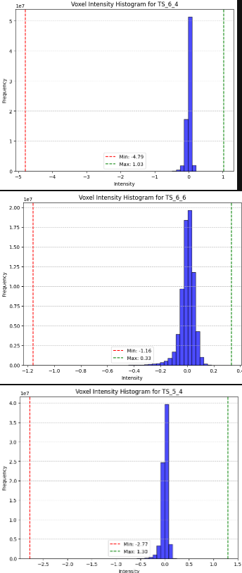\n\n**Data standardized after clipping below**\n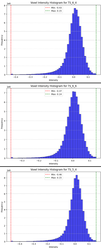\n\n### **Ground Truth Generation**\nI used gaussian heatmaps with radius of 60 for all particles (before scaling to voxel cords). I used the + 0.5 shift identified by @davidlist to set the center of the particle. All of the gaussian were scaled so the max at the center was 1.0 and it decayed from there, regardless of how many particles were in a view. I tried using gaussians defined by the actual radii of the particle of interest, but my models were much more consistent when using a constant radius. A particle size of 60 was chosen based on trial and error of radii that were <= the particle size of apo-ferritin and this seemed to be a sweet spot.\n\n### **Model Architecture**\nI used a 3D U-Net with residual connections on (64,64,64) crops of the data with a 5 channel sigmoidal output. This was partially because I just wanted to to see how well I could do with one. I've always wanted to get into the weeds of using a 3D convnet and I sort of used this competition as an excuse to do just that. It was a lot of fun and I learned a lot by doing it. The parameters for the net were identified with Optuna and shallow networks tended to do better than deeper ones, which was nice given I only had 12 GB of VRAM to fit the model into on my machine. Larger models probably would have forced me into 2D solutions.\n\n### **First Train Set Generation**\nSince this competition was focused on recall, to save compute time I only trained on true positives for the first round of training. I cropped (80,80,80) crops with each particle in an experiment centered in the view to generate at least one view per particle. During training, I augmented with random flips, brightness, and contrast adjustments. I also randomly cropped to the model input size of (64,64,64) to impart a translation augmentation. I tried (48,48,48) and (96,96,96) input sizes as well, but 64 seemed to work the best.\n\n### **Second Train Set Generation**\nAs you might expect, models trained with the dataset prepared as described above were biased towards true positives. This was intentional and I used the resulting models to predict on the entire dataset. I then used the hard false positives as counter examples so the second set was prepared as above + all of the hardest false positives for the original models. This helped with the false positives rate while keeping the false negatives relatively low. It took a lot of fidgeting to get this right and I would like to find a faster, more effective way to find the best thresholds for picking what a useful hard negative would be for this hard negative mining approach to training. I think this was one of the most valuable things I learned to do in this competition and I'd like to work on another problem where I get to refine my approach here.\n\n### **Loss Function**\nI used a custom pixel wise cross entropy loss that used the competition weights and down weighted incorrect predictions where the ground truth was below a threshold to help focus the model to recall. This was a really important part of my solution, but it was admittedly a bit empirical. Conceptually, background was the majority class and I wanted to downweight it, but finding the right downweighting was mostly trial and error. This is another place I think I could have improved my approach, by setting up a framework to systematically evaluate this. I think in the future, if I'm implementing custom losses, I'll need to find better ways to standardize how I evaluate and optimize them.\n\n### **Training**\nI trained my early models using early stopping and reduced the learning rate on plateau. Convergence was a bit tricky at first, but Bayesian Optimization with batch size as one of the variables helped me realize that larger batch sizes typically were unfavorable. I did a little systematic study of 4, 8, 16, and 32 batch sizes and realized that the models weren't converging well with batch sizes > 8. When I used a batch size of 4, I was able to get past this limitation (which was helpful for keeping training on my 3060 in memory anyway). I used per experiment cross validation, starting with 5 experiments for train and 2 experiments for validation. I then switched to 6 experiments for train and 1 experiment for val. This significantly improved my score, which was a little surprising, but it told me that my augmentation was insufficient and more data was helpful for improving generalization. This led me to try and find a training protocol where I could use all 7 experiments. To find the learning rate schedule for these experiments, I fit an exponential curve to the learning rates for each of the 7 models, then used that curve as the learning rate to train on all 7 experiments. The graph below shows a sample of 5 models that each represent a fold of the 7-fold cross validation, as well as the curve that was fit to the average of the learning rates at a given epoch. I trained a 5 seed ensemble using this learning rate schedule and checkpointed the models every 5 epochs, starting at the 40th epoch, then used the public leaderboard (since it tracked so well with my internal validation) to see where the model began to overfit. My final submission was a 5 seed ensemble around the checkpoints at epoch 40.\n\n**Fitted learning rate that was used to train the models trained on the full data**\n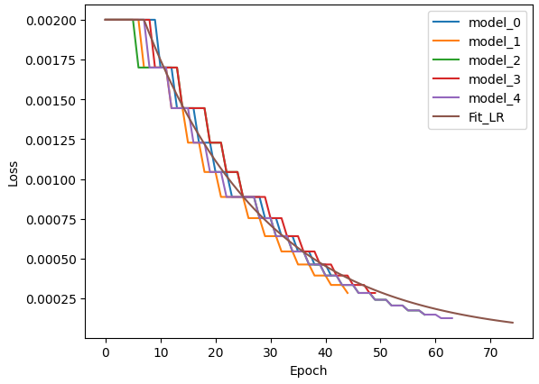\n\n###**Thresholding**\nThe final part of my submission was figuring out how to set the thresholds. I followed a protocol very similar to @hengck23 wherein I used cc3d to find the connected components > 7 voxels, then used the centroid as the submission for a given particle of interest. My models didn't improve much when trying to do things like non-maximum suppression or evaluating the shape of the connected component, so I left them out of my final solution. The real trick was getting the threshold for the particle right. I used a grid search for each particle independently to find the best thresholds. Some of the distributions were peaked and some of the distributions were relatively flat past a certain threshold. On the peaked distributions, I used the maximum value and on the relatively flat ones, I took the leftmost max value, since the problem is biased towards recall. I checked this assumption by scanning the threshold on the public leaderboard for the flatter distributions and I got the best generalization when I chose the leftmost (lowest) threshold.\n\nIf you've read this far, thank you! I really enjoyed competing in this competition and I'm looking forward to the next computer vision competition on Kaggle :).", "votes": 9 } ], "comments": [], "raw_markdown_by_id": { "3117421": "### **Hey everyone!**\n\nThis was a super fun competition I really enjoyed and it's my first silver medal on Kaggle! Thanks to the organizers for a competition on an interesting topic with a cool data set. Also, special thanks to @hengck23 for their discussion posts and connected components workflow, which really helped me get started.\n\n### **Data Preprocessing**\nI clipped the data by percentile (0.99 and 0.01) and standardized per experiment by subtracting the mean of the full voxel grid, divided by the standard deviation. I did this because I noticed that there were some pretty serious outliers. Take a look below at the intensity histograms after standardization with and without clipping. The data looks really consistent from experiment to experiment once the data has been clipped.\n\n**Data standardized without clipping below**\n\n\n**Data standardized after clipping below**\n\n\n### **Ground Truth Generation**\nI used gaussian heatmaps with radius of 60 for all particles (before scaling to voxel cords). I used the + 0.5 shift identified by @davidlist to set the center of the particle. All of the gaussian were scaled so the max at the center was 1.0 and it decayed from there, regardless of how many particles were in a view. I tried using gaussians defined by the actual radii of the particle of interest, but my models were much more consistent when using a constant radius. A particle size of 60 was chosen based on trial and error of radii that were <= the particle size of apo-ferritin and this seemed to be a sweet spot.\n\n### **Model Architecture**\nI used a 3D U-Net with residual connections on (64,64,64) crops of the data with a 5 channel sigmoidal output. This was partially because I just wanted to to see how well I could do with one. I've always wanted to get into the weeds of using a 3D convnet and I sort of used this competition as an excuse to do just that. It was a lot of fun and I learned a lot by doing it. The parameters for the net were identified with Optuna and shallow networks tended to do better than deeper ones, which was nice given I only had 12 GB of VRAM to fit the model into on my machine. Larger models probably would have forced me into 2D solutions.\n\n### **First Train Set Generation**\nSince this competition was focused on recall, to save compute time I only trained on true positives for the first round of training. I cropped (80,80,80) crops with each particle in an experiment centered in the view to generate at least one view per particle. During training, I augmented with random flips, brightness, and contrast adjustments. I also randomly cropped to the model input size of (64,64,64) to impart a translation augmentation. I tried (48,48,48) and (96,96,96) input sizes as well, but 64 seemed to work the best.\n\n### **Second Train Set Generation**\nAs you might expect, models trained with the dataset prepared as described above were biased towards true positives. This was intentional and I used the resulting models to predict on the entire dataset. I then used the hard false positives as counter examples so the second set was prepared as above + all of the hardest false positives for the original models. This helped with the false positives rate while keeping the false negatives relatively low. It took a lot of fidgeting to get this right and I would like to find a faster, more effective way to find the best thresholds for picking what a useful hard negative would be for this hard negative mining approach to training. I think this was one of the most valuable things I learned to do in this competition and I'd like to work on another problem where I get to refine my approach here.\n\n### **Loss Function**\nI used a custom pixel wise cross entropy loss that used the competition weights and down weighted incorrect predictions where the ground truth was below a threshold to help focus the model to recall. This was a really important part of my solution, but it was admittedly a bit empirical. Conceptually, background was the majority class and I wanted to downweight it, but finding the right downweighting was mostly trial and error. This is another place I think I could have improved my approach, by setting up a framework to systematically evaluate this. I think in the future, if I'm implementing custom losses, I'll need to find better ways to standardize how I evaluate and optimize them.\n\n### **Training**\nI trained my early models using early stopping and reduced the learning rate on plateau. Convergence was a bit tricky at first, but Bayesian Optimization with batch size as one of the variables helped me realize that larger batch sizes typically were unfavorable. I did a little systematic study of 4, 8, 16, and 32 batch sizes and realized that the models weren't converging well with batch sizes > 8. When I used a batch size of 4, I was able to get past this limitation (which was helpful for keeping training on my 3060 in memory anyway). I used per experiment cross validation, starting with 5 experiments for train and 2 experiments for validation. I then switched to 6 experiments for train and 1 experiment for val. This significantly improved my score, which was a little surprising, but it told me that my augmentation was insufficient and more data was helpful for improving generalization. This led me to try and find a training protocol where I could use all 7 experiments. To find the learning rate schedule for these experiments, I fit an exponential curve to the learning rates for each of the 7 models, then used that curve as the learning rate to train on all 7 experiments. The graph below shows a sample of 5 models that each represent a fold of the 7-fold cross validation, as well as the curve that was fit to the average of the learning rates at a given epoch. I trained a 5 seed ensemble using this learning rate schedule and checkpointed the models every 5 epochs, starting at the 40th epoch, then used the public leaderboard (since it tracked so well with my internal validation) to see where the model began to overfit. My final submission was a 5 seed ensemble around the checkpoints at epoch 40.\n\n**Fitted learning rate that was used to train the models trained on the full data**\n\n\n###**Thresholding**\nThe final part of my submission was figuring out how to set the thresholds. I followed a protocol very similar to @hengck23 wherein I used cc3d to find the connected components > 7 voxels, then used the centroid as the submission for a given particle of interest. My models didn't improve much when trying to do things like non-maximum suppression or evaluating the shape of the connected component, so I left them out of my final solution. The real trick was getting the threshold for the particle right. I used a grid search for each particle independently to find the best thresholds. Some of the distributions were peaked and some of the distributions were relatively flat past a certain threshold. On the peaked distributions, I used the maximum value and on the relatively flat ones, I took the leftmost max value, since the problem is biased towards recall. I checked this assumption by scanning the threshold on the public leaderboard for the flatter distributions and I got the best generalization when I chose the leftmost (lowest) threshold.\n\nIf you've read this far, thank you! I really enjoyed competing in this competition and I'm looking forward to the next computer vision competition on Kaggle :)." } }